Fast Simulation of Quasistatic Rod Deformations for VR Applications
- 格式:pdf
- 大小:332.96 KB
- 文档页数:7

专利名称:Circuit simulator发明人:トーマス ジー ウィルソン申请号:JP特願2000-611207(P2000-611207)申请日:20000407公开号:JP特表2003-521756(P2003-521756A)A公开日:20030715专利内容由知识产权出版社提供专利附图:摘要: (57)< Abstract > Electronic circuit simulator technology makes the barrier decrease for the simulation of the complicated analog circuit dramatically. As for this invention, before the user which becomes skillful characterizes the system completely the modeling strategy, the deck extraction strategy, and under the test by the fact that it makes that the simulation strategy which can combine the inclusive suit of the design simulation test is formulated possible, setup time is decreased. The design simulationstrategy before this to the is very applied new system fast with automated style by the circuit designer who has the simulation experience which is considerably less than simulation experience of the skill user which formulates the simulation strategy. This invention decreases the CPU time which is needed for each test by making that the skill user encodes the device modeling strategy and the deck extraction strategy which make the CPU time which is necessary in order to achieve specified simulation goal effectively smallest possible. Namely, because of specified simulation goal, the skill user achieves the level of desire of simulation precision vis-a-vis each element which the implement is done in simulation, selects the smallest complex device model which extracts the one part in the complete production schematic which at the same time achieves the level of desire of simulation precision. As for this invention, the effort which is required from the user because the frequency of input which is needed in order to execute the simulation test of specified number is formed is decreased dramatically, the CPU time which is needed in order in addition to execute those is decreased dramatically.申请人:トランシム テクノロジー コーポレイション地址:アメリカ合衆国 オレゴン州 97209 ポートランド エヌダブリュー オーヴァートン 1925ナンバー 201国籍:US代理人:杉村 興作 (外1名)更多信息请下载全文后查看。

AnsysNastranAbaqus Static分析结果⽐较
1. FastModel⾥导⼊⼀个长⽅体
2. 设置边界:长⽅体两端随机设置四点为固定约束,⼀端两点设置为集中⼒荷载X=5, Y=3,如图:
3. 材料库⾥选择⼀种材料
4. Element 属性设置为3D solid。
5. Mesh 属性设置为1阶,Tet 四⾯体Mesh
6. 将有限元模型分别导出为 Ansys,Nastran,Abaqus 格式,并进⾏求解
7. 查看计算结果:
1. Vonmises stress
1.1 Abaqus Stress结果
1.2. Ansys Stress结果
1.3. Nastran Stress结果
2. 位移结果
2.1. Abaqus 位移结果
2.2. Ansys 位移结果
2.3. Nastran位移结果
对于简单的模型,static分析,三软件计算结果完全相同,后续将陆续测试在FastModel中建⽴复杂有限元模型,利⽤ Mesh模块的Size function,测试⽹格质量对结果的影响,以及Ansys/Nastran/Abaqus/Comsol/Radioss 在buckling,
modal,Nonlinear,Thermal 分析的精度⽐较。
有兴趣的朋友可以提供复杂的CAD模型和仿真需求,共同研究。


模拟退火算法模拟退火算法(Simulated Annealing)是一种经典的优化算法,常用于解决复杂的优化问题。
它的灵感来自于金属退火的过程,通过降温使金属内部的不稳定原子重新排列,从而获得更优的结构。
在算法中,通过接受一定概率的差解,模拟退火算法能够逃离局部最优,并最终找到全局最优解。
在MATLAB中,我们可以使用以下步骤来实现模拟退火算法:1.初始化参数:设定初始温度T0、终止温度Tf、温度下降速率α、算法运行的迭代次数等参数,并设定当前温度为T0。
2.生成初始解:根据问题的要求,生成一个初始解x。
3. 迭代优化:在每个温度下,进行多次迭代。
每次迭代,随机生成一个新的解x_new,计算新解的目标函数值f_new。
4. 判断是否接受新解:根据Metropolis准则,判断是否接受新解。
如果新解比当前解更优,则直接接受;否则,以概率exp((f_current - f_new) / T)接受新解。
5.更新解和温度:根据前一步的判断结果,更新当前解和温度。
如果接受了新解,则将新解作为当前解;否则,保持当前解不变。
同时,根据设定的温度下降速率,更新当前温度为T=α*T。
6.重复步骤3-5,直到当前温度小于终止温度Tf。
7.返回最优解:记录整个迭代过程中的最优解,并返回最优解作为结果。
以下是一个简单的示例,演示如何使用MATLAB实现模拟退火算法解决旅行商问题(TSP)。
```matlabfunction [bestPath, bestDistance] =simulatedAnnealingTSP(cityCoordinates, T0, Tf, alpha, numIterations)numCities = size(cityCoordinates, 1);currentPath = randperm(numCities);bestPath = currentPath;currentDistance = calculateDistance(cityCoordinates, currentPath);bestDistance = currentDistance;T=T0;for iter = 1:numIterationsfor i = 1:numCitiesnextPath = getNextPath(currentPath);nextDistance = calculateDistance(cityCoordinates, nextPath);if nextDistance < currentDistancecurrentPath = nextPath;currentDistance = nextDistance;if nextDistance < bestDistancebestPath = nextPath;bestDistance = nextDistance;endelseacceptanceProb = exp((currentDistance - nextDistance) / T); if rand( < acceptanceProbcurrentPath = nextPath;currentDistance = nextDistance;endendendT = alpha * T;endendfunction nextPath = getNextPath(currentPath)numCities = length(currentPath);i = randi(numCities);j = randi(numCities);while i == jj = randi(numCities);endnextPath = currentPath;nextPath([i j]) = nextPath([j i]);endfunction distance = calculateDistance(cityCoordinates, path) numCities = length(path);distance = 0;for i = 1:numCities-1distance = distance + norm(cityCoordinates(path(i),:) - cityCoordinates(path(i+1),:));enddistance = distance + norm(cityCoordinates(path(numCities),:) - cityCoordinates(path(1),:)); % 加上回到起点的距离end```以上示例代码实现了使用模拟退火算法解决旅行商问题(TSP)。

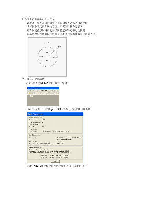
此算例主要用来学习以下方面:针对某一翼型在自由流中以正弦曲线方式振动问题建模此算例中采用两种网格系统,即翼型网格和背景网格针对固定背景网格中的翼型网格建立特定的运动模型运动的翼型网格和固定的背景网格通过嵌套技术实现信息传递第一部分:定常模拟启动CFD-FASTRAN的图形用户界面:选择文件-打开,打开pitch.DTF 文件,点击确认出现下图。
点击“OK”,计算模型的轮廓出现在可视化图形窗口中。
选中控制面板的问题类型栏(PT,如图示):由于我们求解问题使用到Chimera技术,所以在PT栏下除了默认第一项被选中外,还应该选中Overset Meshes(Chimera)。
选中控制面板的模型选项栏(MO),在这里可以设置全局和流动参数。
在Title栏输入:Pitching Airfoil并且选择非轴对称选择Flow分栏设置流动参数:其中,选择理想气体模型并选择湍流模型(求解N-S方程),理想气体特性参数保持默认(分子量和气体常数Gamma),粘性系数计算选择Sutherland公式,普朗特数保持默认不变,选择带壁面修正的K-Epsilon湍流模式。
(具体设置如下)选择控制面板的VC栏设置体条件。
在左下方的窗口选中所有的体,并在控制面板(Properties)将其设置为:Fluid将VC setting mode的第一个下拉菜单设置成Chimera,然后在左下角的窗口中选中zone1和zone2,Chimera下两个下拉菜单分别设置成:yes 和manual specification,这时出现select donor zones,保持两个层参数(过渡层和边缘层)为1,默认不变。
点击select donor zones,在左侧出现zone3,选中zone3后点击OK(图示)。
同理设置zone3,见下图:zone1和zone2为翼型网格,和背景网格zone3存在嵌套关系。
选择控制面板的BC栏设置边界条件:在监视器窗口(左下方)中按住CTRL选中zone1的patch#2,zone2的patch#1将其边界类型设置为Overset,之后点击应用。
simulation modelling practiceSimulation modelling is a crucial tool in the field of science and engineering. It allows us to investigate complex systems and predict their behaviour in response to various inputs and conditions. This article will guide you through the process of simulation modelling, from its basicprinciples to practical applications.1. Introduction to Simulation ModellingSimulation modelling is the process of representing real-world systems using mathematical models. These models allow us to investigate systems that are too complex or expensiveto be fully studied using traditional methods. Simulation models are created using mathematical equations, functions, and algorithms that represent the interactions and relationships between the system's components.2. Building a Basic Simulation ModelTo begin, you will need to identify the key elements that make up your system and define their interactions. Next, you will need to create mathematical equations that represent these interactions. These equations should be as simple as possible while still capturing the essential aspects of the system's behaviour.Once you have your equations, you can use simulation software to create a model. Popular simulation softwareincludes MATLAB, Simulink, and Arena. These software packages allow you to input your equations and see how the system will respond to different inputs and conditions.3. Choosing a Simulation Software PackageWhen choosing a simulation software package, consider your specific needs and resources. Each package has its own strengths and limitations, so it's important to select one that best fits your project. Some packages are more suitable for simulating large-scale systems, while others may bebetter for quickly prototyping small-scale systems.4. Practical Applications of Simulation ModellingSimulation modelling is used in a wide range of fields, including engineering, finance, healthcare, and more. Here are some practical applications:* Engineering: Simulation modelling is commonly used in the automotive, aerospace, and manufacturing industries to design and test systems such as engines, vehicles, and manufacturing processes.* Finance: Simulation modelling is used by financial institutions to assess the impact of market conditions on investment portfolios and interest rates.* Healthcare: Simulation modelling is used to plan and manage healthcare resources, predict disease trends, and evaluate the effectiveness of treatment methods.* Education: Simulation modelling is an excellent toolfor teaching students about complex systems and how they interact with each other. It helps students develop critical thinking skills and problem-solving techniques.5. Case Studies and ExamplesTo illustrate the practical use of simulation modelling, we will take a look at two case studies: an aircraft engine simulation and a healthcare resource management simulation.Aircraft Engine Simulation: In this scenario, a simulation model is used to assess the performance ofdifferent engine designs under various flight conditions. The model helps engineers identify design flaws and improve efficiency.Healthcare Resource Management Simulation: This simulation model helps healthcare providers plan their resources based on anticipated patient demand. The model can also be used to evaluate different treatment methods and identify optimal resource allocation strategies.6. ConclusionSimulation modelling is a powerful tool that allows us to investigate complex systems and make informed decisions about how to best manage them. By following these steps, you can create your own simulation models and apply them to real-world problems. Remember, it's always important to keep anopen mind and be willing to adapt your approach based on the specific needs of your project.。
13 ABAQUS/Explicit准静态分析显式求解方法是一种真正的动态求解过程,它的最初发展是为了模拟高速冲击问题,在这类问题的求解中惯性发挥了主导性作用。
当求解动力平衡的状态时,非平衡力以应力波的形式在相邻的单元之间传播。
由于最小稳定时间增量一般地是非常小的值,所以大多少问题需要大量的时间增量步。
在求解准静态问题上,显式求解方法已经证明是有价值的,另外ABAQUS/Explic it 在求解某些类型的静态问题方面比ABAQUS/Standard更容易。
在求解复杂的接触问题时,显式过程相对于隐式过程的一个优势是更加容易。
此外,当模型成为很大时,显式过程比隐式过程需要较少的系统资源。
关于隐式与显式过程的详细比较请参见第2.4节“隐式和显式过程的比较”。
将显式动态过程应用于准静态问题需要一些特殊的考虑。
根据定义,由于一个静态求解是一个长时间的求解过程,所以在其固有的时间尺度上分析模拟常常在计算上是不切合实际的,它将需要大量的小的时间增量。
因此,为了获得较经济的解答,必须采取一些方式来加速问题的模拟。
但是带来的问题是随着问题的加速,静态平衡的状态卷入了动态平衡的状态,在这里惯性力成为更加起主导作用的力。
目标是在保持惯性力的影响不显著的前提下用最短的时间进行模拟。
准静态(Quasi-static)分析也可以在ABAQUS/Standard中进行。
当惯性力可以忽略时,在ABAQUS/Standard中的准静态应力分析用来模拟含时间相关材料响应(蠕变、膨胀、粘弹性和双层粘塑性)的线性或非线性问题。
关于在ABAQUS/Standard中准静态分析的更多信息,请参阅ABAQUS分析用户手册(ABAQUS Analysis User’s Manual)的第6.2.5节“Quasi-static analysis”。
13.1 显式动态问题类比为了使你能够更直观地理解在缓慢、准静态加载情况和快速加载情况之间的区别,我们应用图13-1来类比说明。
有限元分析软件中Simulation Navigator的使用说明
有限元分析(杭州纳泰科技咨询*************)软件中关于Simulation Navigator的使用:
图1-24 展开的位移节点
∙在Simulation Navigator中,展开SUBCASE — STATIC LOADS 1 Loads。
∙展开Displacement — Nodal。
∙选中Y组元复选框。
显示更新以展示Y位移值,如图1-25所示。
图1-25 Y位移值
第11步退出后置处理器
当完成观察结果时,可以退出后置处理器。
∙在Post Control工具栏上,单击Finish Post Processing图标。
提示:也可以选择Tools→ Results→ Finish Post Processing。
∙关闭所有部件文件。
相关阅读:
排水管及支撑结构强度分析/qiangdujiaohe/195.html
风机轴承与轮毅连接螺栓的强度分析/qiangdujiaohe/196.html
轮船船舶强度分析建模方法的研究/qiangdujiaohe/197.html
转炉壳体有限元法强度分析研究/youxianyuanfenxi/198.html 发电机组法兰联接螺栓的强度分析/qiangdujiaohe/199.html
专业从事机械产品设计│有限元分析│强度分析│结构优化│技术服务与解决方案
本文出自杭州纳泰科技咨询有限公司,转载请注明出处!。
[原创]拟牛顿法Quasi转载须注明出处:在最优化领域,有几个你绝对不能忽略的关键词:拟牛顿、DFP、BFGS。
名字很怪,但是非常著名。
下面会依次地说明它们分别“是什么”,“有什么用”以及“怎么来的”。
但是在进入正文之前,还是要先提到一个概念上的区别,否则将影响大家的理解:其实DFP算法、BFGS算法都属于拟牛顿法,即,DFP、BFGS都分别是一种拟牛顿法。
先从拟牛顿法(Quasi-Newton)说起。
这个怪怪的名词其实很形象:这是一种”模拟“的牛顿法。
那么,它模拟了牛顿法的哪一部分呢?答:模拟的就是牛顿法中的搜索方向(可以叫作“牛顿方向”)的生成方式。
牛顿法是什么?本文是基于你已经知道牛顿法的原理的假设,如果你不清楚,那么可以看我这篇文章,里面非常简单而又清晰地描述了牛顿法的原理。
了解了牛顿法的原理,我们就知道了:在每一次要得到新的搜索方向的时候,都需要计算Hesse矩阵(二阶导数矩阵)。
在自变量维数非常大的时候,这个计算工作是非常耗时的,因此,拟牛顿法的诞生就有意义了:它采用了一定的方法来构造与Hesse矩阵相似的正定矩阵,而这个构造方法计算量比牛顿法小。
这就是对它“有什么用”的回答了。
(1)DFP算法下面,就从DFP算法来看看“拟牛顿”是如何实现的(DFP算法是以Davidon、Fletcher、Powell三位牛人的名字的首字母命名的)。
前面说了,Hesse矩阵在拟牛顿法中是不计算的,拟牛顿法是构造与Hesse矩阵相似的正定矩阵,这个构造方法,使用了目标函数的梯度(一阶导数)信息和两个点的“位移”(X k-X k-1)来实现。
有人会说,是不是用Hesse矩阵的近似矩阵来代替Hesse矩阵,会导致求解效果变差呢?事实上,效果反而通常会变好。
有人又会问为什么?那么就简要地说一下——由牛顿法的原理可知如下几个等式:若最后一个等式子的最左边 < 0,即,就是直观概念上的“沿方向d上,目标函数值下降”的表达。
Fast Simulation of Quasistatic Rod Deformations for VR ApplicationsJ.Linn1,T.Stephan1,J.Carlsson2,and R.Bohlin21Fraunhofer ITWM,Kaiserslautern(linn@itwm.fraunhofer.de)2Fraunhofer–Chalmers Research Center FCC,G¨o teborg(www.fcc.chalmers.se)Summary.We present a model offlexible rods–based on Kirchhoff’s geometrically exact theory–which is suitable for the fast simulation of quasistatic deformations within VR or functional DMU applications.Unlike simple models of“mass&spring”type typically used in VR applications,our model provides a proper coupling of bend-ing and torsion.The computational approach comprises a variational formulation combined with afinite difference discretization of the continuum model.Approxi-mate solutions of the equilibrium equations for sequentially varying boundary condi-tions are obtained by means of energy minimization using a nonlinear CG method. The computational performance of our model proves to be sufficient for the inter-active manipulation offlexible cables in assembly simulation.1IntroductionThe handling offlexible objects in multibody simulation(MBS)models is both a long term research topic[1,2]as well as an active area of current research within the MBS community[3–5].A standard approach supported by most commercial software packages representsflexible bodies by means of vibrational modes(e.g.of Craig–Bampton type[6,7])computed by modal analysis within the framework of linear elasicity.The modal representation of aflexible structure usually yields a drastic reduction of the degrees of freedom and thereby provides a reduced model.However,such methods are suitable (as well as by definition restricted)to model forced oscillations effecting small deformations within aflexible structure.If theflexible bodies of interest possess special geometrical properties char-acterising them as slender(or thin)structures(i.e.rods,plates or shells),their overall deformation in response to moderate external loads may become large, although locally the stresses and strains remain small.Therefore,models suit-able to describe such large deformations of slender structures must be capable to account for geometric pared to object geometries that require fully three-dimensional volume modelling,the reduced dimensional-ity of rod or shell models is accompanied by a considerable reduction in the248J.Linn et al.number of degrees of freedom,which makes the inclusion of appropriately dis-cretised versions of the full models(in contrast to modally reduced ones)into a MBS framework[4]computationally feasible even for time critical simulation applications.Modelling of Flexible Structures in VR ApplicationsThe application aimed at within the framework of this article is the modelling offlexible cables or tubes(e.g.those externally attached to manufacturing robots)such that quasistatic deformations occurring during sufficiently slow motions of these cables can be simulated in real time.This capability is crucial for the seamless integration of a cable simulator module within VR(virtual reality)or FDMU(functional digital mock up)software packages used for interactive simulation(e.g.of assembly processes).Although the dominant paradigm to assess the quality of an animation or simulation within these application areas–as well as related ones like computer games or movies–seems to be“...It’s good enough if it looks good ...”[8],such that a mere“fake”[9]of structure deformation is considered to be acceptable(at least for those applications were“...fooling of the eye ...”[8]is the main issue),the need for“physics based”approaches increases constantly,and the usage of models that are more[12]or less[10,11,13]based on ideas borrowed from classical structural and rigid body mechanics is not uncommon,especially if the primary concern is not visual appearance but physical information(see e.g.[14]).2Cosserat and KirchhoffRod ModelsIn structural mechanics slender objects like cables,hoses,etc.are described by one-dimensional beam or rod models which utilise the fact that,due to the relative smallness of the linear dimension D of the cross-section compared to the length L of a rod,the local stresses and strains remain small and the cross sections are almost unwarped,even if the overall deformation of the rod relative to its undeformed state is large.This justifies kinematical assumptions that restrict the cross sections of the deformed rod to remain plane and rigid.In the following we give brief introduction to rod models of Cosserat and Kirchhofftype,the latter being a special case of the former.We do not present the most general versions of these models,which are discussed at length in the standard references[16]and[18].The approach wefinally use as a basis for the derivation of a generalized“mass&spring”type model byfinite difference discretisation is an extensible variant of Kirchhoff’s original theory[15]as presented in[17](see part II,16–19)for a hyperelastic rod with symmetric cross-section subject to a constant gravitational body force.Fast Simulation of Quasistatic Rod Deformations for VR Applications 2492.1Kinematics of Cosserat and KirchhoffRodsA (special)Cosserat rod [18]is a framed curve [21]formally defined as amapping s →(ϕ(s ),ˆF(s ))of the interval I =[0,L ]into the configuration space R 3×SO(3)of the rod,where L is the length of the undeformed rod.Its constituents are (i)a space curve ϕ:I →R 3that coincides with the line of centroids piercing the cross sections along the deformed rod at their geometri-cal center,and (ii)an “curve of frames”ˆF:I →SO(3)with the origin of each frame ˆF(s )attached to the point x s =ϕ(s ).The matrix representation of the frame ˆF (s )w.r.t.a fixed global coordinate system {e (1),e (2),e (3)}of R 3may be written as a triple of column vectors,i.e.ˆF(s )= d (1)(s ),d (2)(s ),d (3)(s ) ,obtained as d (k )(s )=ˆF(s )·e (k ).By definition d (3)coincides with the unit cross section normal vector located at ϕ(s ).For simplicity we assume the undeformed rod to be straight and prismatic such that its intial geometry relative to {e (1),e (2),e (3)}is given by the direct product A ×I with a constant cross section area A parallel to the plane spanned by {e (1),e (2)}.Introducing coordinates (ξ1,ξ2)in the plane of the cross section A relative to its geometrical center,we may parametrise the material points X ∈A ×I of the undeformed rod geometry by X (ξ1,ξ2,s )= k =1,2ξk e (k )+s e (3),and the deformation mapping X →x =Φ(X )is given by the formula x (ξ1,ξ2,s )=ϕ(s )+ k =1,2ξk d (k )(s ).The kinematics of a framed curve as presented above determine the possible deformations of a Cosserat rod.These are stretching (in the direction of the curve tangent),bending (around an axis in the plane of the cross section),twisting (of the cross section around its normal)and shearing (i.e.tilting of the cross section normal w.r.t.the curve tangent).Following Chouaieb and Maddocks [21]we denote a frame ˆF(s )as adapted to the curve ϕ(s )if d (3)(s )coincides with the unit tangent vector t (s )=∂s ϕ(s )/ ∂s ϕ(s ) along the curve.An adapted frame satisfies the Euler–Bernoulli hypothesis,which states that the cross sections remain always or-thogonal to the centerline curve in a deformed state also.Curves with adapted frames describe the possible deformations of (extensible)Kirchhoff-pared to Cosserat rods the kinematics of Kirchhoffrods are further restricted,as they do not allow for shear deformations.The inextensibiliy condition ∂s ϕ =1constitutes an additional kinematical restriction.Measuring the slenderness of a rod of cross-section diameter D and length L in terms of the small parameter ε=D/L and assuming (hyper)elastic ma-terial behaviour one may show that the potential energy terms corresponding to bending and torsion are of the order O (ε4),while the energy terms corre-sponding to stretching and shearing scale are of the order O (ε2).In this way the latter effectively act as penalty terms that enforce the kinematical restric-tions ∂s ϕ =1and d (3)(s )=t (s ).This explains how Kirchhoffrods appear as a natural limit case of Cosserat rods subject to moderate deformations provided εis sufficiently small.250J.Linn et al.2.2Hyperelastic KirchhoffRods with Circular Cross-SectionAs we are interested in a rod model that is suitable for the simulation of mod-erate cable deformations,both the Cosserat as well as the Kirchhoffapproach wouldfit for our purpose.A characteristic feature of the Cosserat model con-sists in the description of the bending and torsion of the rod in terms of the frame variables,while the bending of the centerline curveϕ(s)is produced only indirectly via shearing forces that try to align the curve tangent to the cross section normal.In contrast to that,Kirchhoff’s model[20]encodes bend-ing strain directly by the curvature ofϕ(s)and therefore provides a direct pathway to mass&spring type models formulated in terms of(discrete)dof of the centerline.Averaging the normal Piola–Kirchhofftractions and corresponding torques over the cross-section surface of the deformed rod located atϕ(s)yields stress resultants f(s)and stress couples m(s),i.e.resultant force and moment vectors per unit reference length[19].If the rod is in a static equilibrium state,these vectors satisfy the differential balance equations of forces and moments∂s f+G=0,∂s m+∂sϕ×f=0,(1) where G represents a(not necessarily constant)body force acting along the rod,and we assumed that no external moment is applied in between the rod boundaries.In the case of an extensible Kirchhoffrod which in its undeformed state has the form of a straight cylinder with circular cross section,the assumption of a hyperelastic material behaviour yields the expression[17]m(s)=EI t(s)×∂s t(s)+GJΩt t(s)(2) for the stress couple,where E is Young’s modulus,G is the shear modulus,I measures the geometrical moment of inertia of the cross section(I=π4R4for a circular cross section of radius R)and J=2I.The quantities EI and GJ determine the stiffness of the rod w.r.t.bending and torsion.The strain measure related to the bending moment is given by the vectort×∂s t=∂sϕ×∂2sϕ∂sϕ 2= ∂sϕ κb(3)which is proportional to the Frenet curvatureκ(s)of the centerline and(if κ>0)points in the direction of the binormal vector b(s).The strain measure related to the torsional moment is determined by the twistΩt(s)=t(s)·[d(s)×∂s d(s)],(4) where d(s)is any unit normal vectorfield to the centerline given as afixed linear combination d=cos(α0)d(1)+sin(α0)d(2)of the frame vectors d(1)(s) and d(2)(s)for some constant angleα0.Note that the special constitutive relation(2)implies that in equilibrium the twistΩt is constant.Fast Simulation of Quasistatic Rod Deformations for VR Applications251 As a Kirchhoffrod is(by definition)unshearable,only the tangential com-ponent of the stress resultant f(s)is constitutively determined by the tension t(s)·f(s)=:T(s)=EA( ∂sϕ −1)(5) related to the elongational strain( ∂sϕ −1).The resistance of the rod w.r.t.stretching is determined by EA where A=|A|is the size of the cross-section area(in our case A=πR2).The shearing force acting parallel to the cross section is given by f sh(s)=f(s)−T(s)t(s).It is not related to any strain measure but has to be determined from the equilibrium equations a Lagrange parameter corresponding to the internal constraint d(s)·t(s)=0.To determine the deformation of the rod in static(or likewise quasistatic) equilibrium one has to solve the combined system of the equations(1)–(5)for a suitable set of boundary conditions,e.g.like those discussed in[20].(This issue will not be discussed here.)Equivalently,one may obtain the centerline ϕ(s)and the unit normal vectorfield d(s)that represents the adapted frame of the rod by minimization of the potential energyW pot[ϕ,d]=L0w el(s)d s−LG(s)·ϕ(s)d s.(6)According to(2)–(5)the elastic energy density is a quadratic form in the various strain measures given byw el(s)=EI2(t×∂s t)2+GJ2Ω2t(s)+EA2( ∂sϕ −1)2(7)and determines the stored energy function W el[ϕ,d]= Lw el(s)d s contain-ing the internal part of W pot.A specific choice of boundary conditions may be accounted for by modified expressions for w el(0)and w el(L),which are obtained from(7)byfixing combinations of the kinematical variablesϕ(s) and d(s)and their derivatives at prescribed values(as required by the b.c.) and substituting these into w el(s).3Discrete Rod Models of“Mass&Spring”TypeThefinal step of our approach towards a model offlexible rods suitable for the fast computation of quasistatic rod deformations is the discretisation of the potential energy by applying standard(e.g.central)finite difference stencils to the elastic energy density(7)and corresponding quadrature rules(e.g.trape-zoidal)to the energy integrals(6).(Boundary conditions are treated in the way described at the end of the previous section.)This procedure results in a discrete model of an extensible Kirchhoffrod that has a similar structure like the simple“mass&spring”type models presented in[11]and[13].However,as a benefit of the systematic derivation252J.Linn et al.procedure on the basis of a proper continuum model,our discrete rod model is able to capture the rather subtle coupling of bending and torsion deformation.We compute approximate solutions of the equilibrium equations for se-quentially varying boundary conditions by a minimization of the discrete po-tential energy using a nonlinear CG method[22].The computational efficiency of our approach is illustrated by the typical results shown in Fig.1above. As the calculation times are comparable to those mentioned in Gregoire and Schomer[13],we estimate that our model is suitable for the interactive manip-ulation offlexible cables in assembly simulation(as indicated by preliminary tests with a software package developped at FCC.)Fig.1.Sequential deformation of a discrete,hyperelastic Kirchhoffrod of symmetric cross section:(a)Starting from a circle segment,the tangents of the boundary frames are bent inward to produce(b)an(upside down)Ω-shaped deformation of the rod at zero twist.To demonstrate the effect of mutual coupling of bending and torsion in the discrete model,the boundary frame at s=L is twisted counterclockwise by an angle of2πwhile the other boundary frame at s=0is heldfixed.The pictures(c)–(f)show snapshots of the deformation state taken at multiples ofπ/2. The overall deformation from(a)–(f)was split up into a sequence of25consecutive changes of the boundary conditions defined by the terminal frames of the rod.For a discretization of the cable into10segments,the simulation took150ms on1CPU of an AMD2.2GHz double processor PC,which amounts to an average computation time of6ms per stepFast Simulation of Quasistatic Rod Deformations for VR Applications253 References1.W.O.Schiehlen:Multibody system dynamics:Roots and perspectives,MultibodySystem Dynamics1,p.149–188(1997)2. A.A.Shabana:Flexible multibody dynamics:Review of past and recent devel-opments,Multibody System Dynamics1,p.189–222(1997)3. B.Simeon:Numerical Analysis of Flexible Multibody Systems,Multibody Sys-tem Dynamics6,p.305–325(2001)4.P.Betsch:Computational Methods for Flexible Multibody Dynamics,Habilita-tionsschrift(2002)5. A.A.Shabana:Dynamics of Multibody Systems(Third edition),Cambridge Uni-versity Press(2005)6.R.R.Craig Jr.and M.C.C.Bampton:Coupling of Substructures for DynamicAnalysis,AIAA Journal Vol.6,No.7,July19687.R.R.Craig:Structural Dynamics,Wiley(1981)8. D.Roble and T.Chan:Math in the Entertainment Industry,p.971–990inB.Engquist and W.Schmidt(ed.):Mathematics Unlimited—2001and Beyond,Springer(2001)9.R.Barzel:Faking dynamics of ropes and springs,IEEE Comput.Graph Appl.17(3),p.31–39(1996)10. D.Baraffand A.Witkin:Large steps in cloth simulation,p.43–54in Proceedingsof SIGGRAPH98,Computer Graphics Proceedings ed.by M.Cohen,Addison Wesley(1998)11. A.Look and E.Sch¨o mer:A virtual environment for interactive assembly simu-lation:from rigid bodies to deformable cables,in5th World Multiconference on Systemics,Cybernetics and Informatics(SCI’01),Vol.3(Virtual Engineering and Emergent Computing),p.325–332(2001)12. D.K.Pai:Strands:Interactive simulation of thin solids using Cosserat models,Comput.Graph.Forum21(3),p.347–352(2002)13.M.Gregoire and E.Sch¨o mer:Interactive simulation of one-dimensional felxibleparts,ACM Symposium on Solid and Physical Modeling(SPM’06),p.95–103 (2006)14.H.Baaser:L¨a ngenoptimierung von Bremsschl¨a uchen und deren FE–Analyse aufMikroebene,VDI–Berichte Nr.1967,p.13–22(2006)15.G.Kirchhoff:¨Uber das Gleichgewicht und die Bewegung eines unendlich d¨u nnenelastischen Stabes,J.Reine Angew.Math.(Crelle)56,p.285–343(1859) 16. A.E.H.Love:A Treatise on the Mathematical Theory of Elasticity(4th edition),Cambridge University Press(1927),reprinted by Dover(1944)ndau and E.M.Lifshitz:Theory of Elasticity(Course of TheoreticalPhysics,Vol.7,3rd edition),Butterworth Heinemann(1986)18.S.Antman:Nonlinear Problems of Elasticity(2nd Edition),Springer(2005)19.J.C.Simo:Afinite strain beam formulation:the three dimensional dynamicproblem–Part I,Comp.Meth.Apl.Mech.Eng.49,p.55–70(1985)20.J.H.Maddocks:Stability of nonlinearly elastic rods,Arch.Rational Mech.&Anal.85,p.311–354(1984)21.N.Chouaieb and J.H.Maddocks:Kirchhoff’s problem of helical equilibria ofuniform rods,J.Elasticity77,p.221–247(2004)22.J.R.Shewchuck:An Introduction to the Conjugate Gradient Method Withoutthe Agonizing Pain,/jrs/(1994)。