Transpiration response to soil moisture in pine and spruce trees in Sweden
- 格式:pdf
- 大小:413.50 KB
- 文档页数:19

土壤饱和含水率英文Soil Saturation Moisture ContentSoil is a crucial component of the Earth's surface, playing a vital role in supporting various ecosystems and human activities. One of the fundamental properties of soil is its moisture content, which is a measure of the amount of water present in the soil. The soil saturation moisture content, also known as the soil saturation point, is a crucial parameter that determines the maximum amount of water that a soil can hold before becoming saturated.Understanding the soil saturation moisture content is essential for various applications, including agriculture, civil engineering, and environmental management. In agriculture, it helps farmers determine the appropriate irrigation schedules and ensure optimal plant growth. In civil engineering, it is crucial for assessing the stability of soil structures, such as foundations and slopes. In environmental management, it is essential for understanding the water cycle, predicting flood risks, and managing water resources.The soil saturation moisture content is influenced by several factors, including soil texture, soil structure, and the presence of organicmatter. Soil texture refers to the relative proportions of sand, silt, and clay particles in the soil. Sandy soils, for example, have larger pore spaces and tend to have a lower saturation moisture content compared to clay soils, which have smaller pore spaces and can hold more water.Soil structure, on the other hand, refers to the arrangement of soil particles and the formation of aggregates. Well-structured soils with good aggregation tend to have a higher saturation moisture content due to the presence of larger pore spaces. Organic matter in the soil also plays a crucial role in increasing the soil's water-holding capacity, as it can absorb and retain moisture more effectively than mineral soil particles.To measure the soil saturation moisture content, various methods can be used, including laboratory analysis, field measurements, and remote sensing techniques. Laboratory analysis involves taking soil samples and determining the moisture content using gravimetric or volumetric methods. Field measurements can be performed using soil moisture sensors, which measure the electrical conductivity or dielectric properties of the soil to estimate the moisture content.Remote sensing techniques, such as satellite or aerial imagery, can also be used to estimate the soil moisture content over larger areas. These methods rely on the relationship between the soil's reflectanceor emissivity and its moisture content, and they can provide valuable information for large-scale applications, such as regional water management or drought monitoring.Once the soil saturation moisture content is known, it can be used to inform various decisions and management practices. In agriculture, the information can be used to optimize irrigation schedules, reduce water waste, and improve crop yields. In civil engineering, it can be used to assess the stability of soil structures and inform the design of foundations, slopes, and other infrastructure.In environmental management, the soil saturation moisture content is crucial for understanding the water cycle and predicting the occurrence of floods and droughts. It can also be used to inform the management of water resources, such as the allocation of water for different uses and the implementation of conservation measures.In conclusion, the soil saturation moisture content is a fundamental property of soil that has far-reaching implications for various applications. Understanding and accurately measuring this parameter is essential for effective soil and water management, as well as for addressing the challenges posed by climate change and other environmental factors. By leveraging the knowledge and tools available, we can better manage our soil and water resources, ensuring their sustainability for generations to come.。

北京山区农田土壤有机质对土壤呼吸的影响研究董士伟;李红;张微微;刘晓娜【摘要】以北京山区为例,首先采用LI-8100开路式土壤碳通量测量系统测定土壤呼吸速率,同时采集土壤样品测定土壤有机质含量;其次对土壤呼吸与土壤有机质的关系进行分析研究,并从不同有机质等级和不同种植类型两个层面对农田土壤呼吸速率进行特征分析,以揭示农田土壤有机质与土壤呼吸的关系.结果表明,北京山区农田土壤有机质含量对土壤呼吸速率有显著影响,二者呈现对数关系,土壤呼吸速率与有机质等级正相关;不同种植类型下农田土壤呼吸速率不同,玉米最高,大豆次之,花卉最低.【期刊名称】《湖北农业科学》【年(卷),期】2015(054)020【总页数】3页(P4982-4984)【关键词】土壤呼吸;有机质;农田;特征分析;北京山区【作者】董士伟;李红;张微微;刘晓娜【作者单位】北京市农林科学院农业综合发展研究所,北京100097;北京市农林科学院农业综合发展研究所,北京100097;北京市农林科学院农业综合发展研究所,北京100097;北京市农林科学院农业综合发展研究所,北京100097【正文语种】中文【中图分类】S154土壤呼吸过程是陆地生态系统碳循环中土壤碳的主要输出途径,是大气CO2重要排放源,其排放量是陆地生态系统向大气排放碳的最大通量之一[1]。
农业是重要的温室气体来源,土壤中的有机物质经微生物分解,以CO2的形式释放入大气。
许多研究表明,土壤温度、水分和有机质的变化是造成土壤呼吸有明显日变化和季节变化规律的重要原因[2-5]。
虽然很多研究者在这些方面做了大量工作,但各个因素作用于土壤呼吸的影响机理和作用大小尚不明确,不同环境影响因子所起的作用也不同。
土壤有机质能促使土壤形成结构,改善土壤物理、化学及生物学过程,对CO2影响最显著,为此从土壤有机质角度出发,系统研究了农田土壤有机质含量对土壤呼吸速率的影响。
1 研究区概况与研究方法1.1 研究区概况北京山区位于北京市西部、北部和东北部,地处东经115°24′~117°30′,北纬39°38′~41°05′。
土壤学中英文对照名词土壤soil 陆地表面由矿物质、有机物质、水、空气和生物组成,具有肥力,能生长植物的未固结层。
土壤学soil science 研究土壤的形成、分类、分布、制图和土壤的物理、化学、生物学特性、肥力特征以及土壤利用、改良和管理的科学。
发生土壤学pedology 侧重研究土壤的发生、演化、特性、分类、分布和利用潜力的土壤学。
耕作土壤学edaphology 侧重研究土壤的组成、性质及其与植物生长的关系,通过耕作管理提高土壤肥力和生产能力的土壤学.土壤地理[学]soil geography 研究土壤的空间分布和组合及其地理环境相互关系的学科.土壤物理[学] soil physics 研究土壤中物理现象或过程的学科。
土壤化学soil chemistry 研究土壤中各种化学行为和过程的学科。
土壤生物化学soil biochemistry 阐明土壤有机碳和氮素等物质的转化、消长规律及其功能的学科.土壤矿物学soil mineralogy 研究土壤中原生矿物和次生矿物的类型、性质、成因、转化和分布的学科。
01.011 土壤分析化学soil analytical chemistry 研究用化学方法和原理测定土壤成分和性质的技术学科. 01。
012 土壤生物学soil biology 研究土壤中生物的种类、分布、功能及其与土壤和环境间相互关系的学科.01.013 土壤微生物学soil microbiology 研究土壤中微生物种类、功能和活性以及与土壤和环境间相互关系的学科。
01.014 土壤生态学soil ecology 研究土壤环境与生物间相互关系,以及生态系统内部结构、功能、平衡与演变规律的学科。
01.015 土壤微形态[学]soil micromor—phology 研究土壤显微形态特征的学科.01。
016 土壤资源soil resources 土壤类型的数量与质量。
01.017 土壤区划soil regionalization 按土壤群体的地带性和地域性差异进行分区划片,提出开发利用途径。
基于Landsat 8遥感图像的土壤含水量提取研究崔丽霞;王蕾【摘要】Soil moisture is not only a major factor in the growth of vegetation,but also an impor-tant parameter in the study of climate,water temperature,ecology,agriculture and many other fields.Remote sensing can quickly and easily get the surface information of a large area,so it is very important to use remote sensing technology to extract soil moisture content.In this essay, with Landsat 8 images of August 15,2015 in north central of Tangshan as the research object,the soil moisture distribution of the region is obtained by calculating the normalized vegetation index and inverting the land surface temperature.The research results show that the vegetation water supply index method can be used to extract the information of the soil moisture content of Land-sat 8 remote sensing images,which extends the application range of Landsat 8 images.%土壤含水量是影响植被生长的一个主要因素,也是研究气候、水温、生态、农业等领域的重要参数。
- 1 -田间土壤含水率测量的几种主要方法1林剑辉 孙宇瑞※ 马道坤中国农业大学精细农业研究中心,北京,100083摘 要:土壤含水率是农业生产中一重要参数,本文对土壤水分的各种测量方法进行了全面的综合介绍。
首先讨论了称重法,张力计法,电阻法,中子法,r-射线法,驻波比法,时域反射击法及光学法等的基本原理。
其次由于土壤含水率受土壤质地,容重,含盐量,温度等影响,因此各种测量方法在实地测量时均会产生误差,本文紧接着详细分析了各种方法使用过程中产生误差的主要原因,并提出了相应的补偿措施。
最后,通过对这些方法的对比分析,得出了一些结论,并提出了土壤水分测量方法进一步研究的重点。
关键词:土壤含水率、传感器、测量1. 引言水乃生命之源,对于农作物而言,土壤水更是其发育、生长的重要条件。
在古中国农业中,将湿润的土壤称为“墒”,并有丰富的关于保墒、散墒等调节土壤水分状况(墒情)的技术和作业。
在现代农业中,能否对土壤水分进行有效测量与控制,是实现“精细农业”与“精细灌溉”的关键所在。
同时在水文科学、气象科学和生态科学中,土壤水分的测量也具有相当重要的意义。
土壤中水分含量称之为土壤含水率(Soil Moisture Content),是由土壤三相体(固相骨架、水或水溶液、空气)中水分所占的相对比例表示的,通常采用重量含水率(g θ)和体积含水率(v θ)两种表示方法[1]。
重量含水率是指土壤中水分的重量与相应固相物质重量的比值,体积含水率是指土壤中水分占有的体积和土壤总体积的比值。
体积含水率与重量含水率两都之间可以换算:c g v γθθ=,其中c γ为土壤干容重。
而Reynolds(1970)指出,采用体积含水率是克服土壤变异性对土壤含水率测量的影响的一种有效方法[2]。
由于作为水载体的土壤是一种多孔介质,物理化学特性复杂,空间变异性大,这些给土壤含水率的测量提出了很高的技术要求。
半个多世纪以来,科研人员针对这种状况,采用了不同的方法进行土壤水分测量的研究,各种测量技术也层出不穷。


间接推求非饱和土壤导水参数的方法【摘要】本文介绍了四种间接推求非饱和土壤导水参数的方法,包括土壤水分再分布过程法、土壤水分特征曲线拟合模型法、简单入渗法和土壤转换函数法,并对四种方法出归纳,提出了进一步研究的方向。
【关键词】非饱和土壤导水参数;水分再分布;水分特征曲线;简单入渗法;PTFs确定非饱和土壤导水参数的方法有两大类:直接法和间接法。
鉴于直接法,耗时多,价格昂贵,所得精度难以保证,空间差异性大,间接法成为许多专家学者研究的焦点。
本文通过介绍推求非饱和土壤导水参数的主要几种间接方法,做出归纳,以期为非饱和土壤导水参数间接法的进一步研究起到推动作用。
1.土壤水分再分布过程法邵明安[1]提出的一种土壤导水参数模型,将一维垂直和水平土壤水分再分布过程结合起来,根据土壤湿润锋湿度与湿润剖面平均湿度之间的函数关系,推出非饱和导水率K(θ)的解析表达式。
这样,只要利用土壤水分再分布的湿润过程,确定表达式中的常数,就可直接算出土壤的非饱和导水率。
根据湿润锋湿度与平均湿度拟合关系的不同,推出K(θ)有不同的表达式,本文采用湿润锋湿度与平均湿度为幂函数关系:K(θ)=(θ-θinm■■-Z■■-n■m■■■-X■■)上式:θ为体积含水率,θi为初始含水率,H为水深,Z、X分别为垂直和水平方向水分运移的距离,Z■和X■为所加其水面刚刚消失时初始湿润深度,m、n、m1、n1、a、b均为拟合参数。
2.土壤水分特征曲线拟合模型法2.1 Mualem模型Mualem模型关于相对导水率的表达式如下:Kr(Θ)=Θ1/2■■/■■■(1)式中:Kr为相对导水率,即K/Ks,h为水头值,Θ为无量纲含水量。
无量纲含水量表达式Θ=■(2)求解方程(1)时需要建立无量纲含水量与水头值的关系式,采用幂函数形式:Θ=(ah)-b(3)将(3)式代入方程(1)积分得:Kr(Θ)=Θ5/2+2/b(4)2.2 Burdine模型Burdine建立的相对导水率表达式如下:Kr(Θ)=Θ2■■/■■(5)将(3)式代入方程(5)积分得:Kr(Θ)=Θ3+2/b(6)2.3 Van Genuchten模型[2]Van Genuchten水分特征曲线模型为:Θ=[1+(ah)n]-m(7)式中:α是标定参数,与土壤平均孔隙半径成正比,n和m是土壤水分特征曲线的形状参数或孔隙分布指数,且有m=1-1/n。

测定土壤饱和渗透系数的试验方法与结果优化吕杰;陈植华;龚星【摘要】土的渗透系数是一个极其重要的水文地质参数,它反映了土壤和岩层的透水性能,是地下水计算中一个不可缺少的指标,但土的渗透试验受诸多因素的影响,如土的物理性质、试验环境、试验场所、人为操作等.为了较为客观、准确地获取包气带浅层土壤饱和渗透系数,本文概述了Guelph渗透仪法野外渗透试验和室内变水头渗透试验测定土壤饱和渗透系数的原理与方法,并通过统计学中的置信区间对试验数据进行了优化处理.结果表明:野外试验测得的土壤饱和渗透系数较室内试验大,但误差在一个数量级内;室内试验测得的土壤饱和渗透系数与《工程地质手册》(第三版)给出的土壤饱和渗透系数参考值接近;Guelph渗透仪用于野外测定土壤饱和渗透系数的可靠性较高.【期刊名称】《安全与环境工程》【年(卷),期】2013(020)005【总页数】6页(P144-148,162)【关键词】土壤;饱和渗透系数;Guelph渗透仪法;室内渗透试验;置信区间;可靠性【作者】吕杰;陈植华;龚星【作者单位】中国地质大学研究生院,武汉430074;中国地质大学环境学院,武汉430074;中国地质大学研究生院,武汉430074【正文语种】中文【中图分类】TU411.4土的渗透系数取决于土的物理性质(如颗粒组成、颗粒形状、孔隙比以及土的结构等)和土体中水的物理性质(如水的黏滞性、水中可溶盐含量等)。
土壤渗透系数的测定方法可分为室内测定法和野外测定法两类[1],但由于影响土壤渗透系数的因素十分复杂,而目前室内和野外所测定的土壤渗透系数是个粗略的数值,因此土壤渗透系数的测定方法仍处于不断的研究与改进之中。
目前土壤渗透系数的野外测定方法较多,如双环法、渗透仪法、人工模拟降雨法、土柱法、钻孔法、稳定通量法以及渗透桶法等[2,3],但最常用的是双环法,Guelph渗透仪法应用较少。
在诸多野外测定土壤渗透系数的方法中,Guelph渗透仪法具有快速简便、耗水少、试验时间短(一般仅为5 min~1 h)等特点,但由于试验数据的有效性偏低,因此为了达到取样精度与置信水平,需要进行多点多组试验。

去除调落物对马尾松人工林土壤呼吸的影响摘要:文章采用去除调落物法来研究土壤呼吸通量的变化,结果表明:土壤CO2释放月平均变化动态基本上呈单峰值曲线。
对照和去除调落物的土壤呼吸速率均呈现显著的季节性变化,对照的土壤呼吸速率变化范围为 1.352~5.865μmol•m-2s-1,而去除调落物的土壤呼吸速率范围为 1.435~5.754μmol•m-2s-1,去除调落物的土壤呼吸速率与5cm土壤温度之间均呈显著指数相关(P=0.000),5cm土壤湿度相关分析表明,相关关系显著(P=0.012)。
去除凋落物和对照处理土壤呼吸的温度敏感系数Q10值分别为2.5和2.7,其去除凋落物的Q10值<对照的Q10值。
由此说明根系是影响CO2通量,温度,湿度一个重要因子。
关键词:土壤呼吸;马尾松人工林;温度;湿度;Q10值;土壤呼吸是在土壤新陈代谢功能过程中,产生大量的二氧化碳,并向大气释放二氧化碳的过程。
它包括微生物的呼吸、根系的呼吸和地下动物的呼吸三个生物过程,以及一个非生物过程:即在高温条件下的化学氧化过程[4-6]。
据IPCC(1990年)公布的数据,大气中CO2浓度现正呈上升趋势,到2030年前后,空气中CO2浓度将会达到550μL/L,为产业革命前的2倍[1]。
土壤是一个巨大的碳库,土壤碳库微小的变化可能导致大气CO2浓度的变化[2],森林是陆地生态系统的主要的组成部分,可见,森林土壤有机碳在全球碳平衡中具有重要的地位,研究森林土壤呼吸对于探讨全球CO2变化及其影响,具有十分重要的意义。
本文中对马尾松人工林不同处理过的样地CO2释放量进行定位研究,目的在于揭示马尾松人工林林地CO2释放量生态因子之间可能的联系,从而为气候变暖研究提供中国亚热带森林生态系统方面的基础实验数据。
一、试验地概况本文研究样地位于湖南省浏阳市马尾松培育基地,森林覆盖率90%。
海拔50~106 m。
Temperature sensitivity of soil respiration in different ecosystems in ChinaShushi Peng,Shilong Piao *,Tao Wang,Jinyu Sun,Zehao ShenDepartment of Ecology,College of Urban and Environmental Sciences,and Key Laboratory for Earth Surface Processes of the Ministry of Education,Peking University,Beijing 100871,Chinaa r t i c l e i n f oArticle history:Received 9May 2008Received in revised form 13October 2008Accepted 16October 2008Available online 14November 2008Keywords:Carbon cycle China Climate Q 10Soil respirationTemperature sensitivitya b s t r a c tUnderstanding the sensitivity of soil respiration to temperature change and its impacting factors is an important base for accurately evaluating the response of terrestrial carbon balance to future climatic change,and thus has received much recent attention.In this study,we synthesized 161field measure-ment data from 52published papers to quantify temperature sensitivity of soil respiration in different Chinese ecosystems and its relationship with climate factors,such as temperature and precipitation.The results show that the observed Q 10value (the factor by which respiration rates increase for a 10 C increase in temperature)is strongly dependent on the soil temperature measurement depth.Generally,Q 10significantly increased with the depth (0cm,5cm,and 10cm)of soil temperature measuring point.Different ecosystem types also exhibit different Q 10values.In response to soil temperature at the depth of 5cm,alpine meadow and tundra has the largest Q 10value with magnitude of 3.05Æ1.06,while the Q 10value of evergreen broadleaf forests is approximately half that amount (Q 10¼1.81Æ0.43).Spatial correlation analysis also shows that the Q 10value of forest ecosystems is significantly and negatively correlated with mean annual temperature (R ¼À0.51,P <0.001)and mean annual precipitation (R ¼À0.5,P <0.001).This result not only implies that the temperature sensitivity of soil respiration will decline under continued global warming,but also suggests that such acclimation of soil respiration to warming should be taken into account in forecasting future terrestrial carbon cycle and its feedback to climate system.Ó2008Elsevier Ltd.All rights reserved.1.IntroductionSoil respiration is a major process controlling carbon loss from terrestrial ecosystems.On a global scale,soil respiration was esti-mated to produce 80.4Pg C y À1(petagram carbon per year)with a range of 79.3–81.8Pg C y À1(Raich et al.,2002),accounting for 60–90percent of total respiration of global terrestrial ecosystems (Schimel et al.,2001),which is more than 11times the current rate of fossil fuel combustion (Marland et al.,2000).Accordingly,small changes in the magnitude of soil respiration could have a large effect on the concentration of CO 2in the atmosphere.For example,a recent study suggested that autumnal atmospheric CO 2zero-crossing date has significantly advanced due to the stimulation of soil respiration driven by rising temperature in the Northern Hemisphere (Piao et al.,2008).Several factors can profoundly influence soil respiration,such as soil quality,N deposition,climate condition,and human distur-bance (Davidson and Janssens,2006;Davidson et al.,2006;Mo et al.,2008;Qi et al.,2002).Among these factors,climate change,particularly global warming has been suggested to be the major cause of accelerating global soil carbon loss (Jones et al.,2003).Such increase in soil respiration in response to rising temperature is expected to provide a positive feedback to global warming (Cox et al.,2000;Jenkinson et al.,1991;Raich and Schlesinger,1992),but there are large uncertainties in the magnitude of this feedback (Friedlingstein et al.,2006).Our current poor understanding of the temperature sensitivity of soil respiration is one of the major sources of the uncertainty estimated by different climate–carbon coupling models (Fierer et al.,2006;Jones et al.,2003;Lenton and Huntingford,2003).For example,terrestrial carbon models such as Roth-C,CENTURY and TEM generally assume a constant tempera-ture sensitivity of soil respiration regardless of the characteristics of the ecosystems (Jenkinson et al.,1991;Tian et al.,1999),although a previous study suggested that Q 10,the factor by which soil respiration increases with a 10 C rise in temperature,is likely to*Corresponding author.Department of Ecology,Peking University,Haidian district,Beijing 100871,China.Tel.:þ861062765578;fax:þ861062756560.E-mail address:slpiao@ (S.L.Piao).Contents lists available at ScienceDirectSoil Biology &Biochemistryjournal hom epa ge:/locate/soilbio0038-0717/$–see front matter Ó2008Elsevier Ltd.All rights reserved.doi:10.1016/j.soilbio.2008.10.023Soil Biology &Biochemistry 41(2009)1008–1014vary across different ecosystems and climatic conditions (Raich and Schlesinger,1992).China has climate regimes ranging from perennial snow on the high western mountains to deserts in the western lowlands,and from cold temperate regions in the northwest to warm and humid tropics along the southern coast (Fang et al.,2001a ).The different climates support a set of ecosystems ranging from the boreal coniferous forest in the northeast to the tropical monsoon rain forest in the south.Such wide climatic variability,topographic complexity,and natural ecosystem diversity have provided a unique field for examining temperature sensitivity of soil respi-ration for different ecosystems and climatic conditions.During the last 10years,the number of studies of soil respiration sensitivity to temperature has increased rapidly in China (Fig.1).According to these field measurements,temperature sensitivity of soil respira-tion in China varies from the Q 10value of 0.93for the cropland in Shenyang city,Liaoning Province (Wang et al.,2006b )to that of 6.27for the evergreen needleleaf forest in Li county,Sichuan Province (Chen et al.,2007).Although these previous studies have signifi-cantly improve our understanding on temperature sensitivity of soil respiration at the site level,the sensitivity of soil respiration to temperature at the country and regional scale is not still clear.This insufficient knowledge further limits our ability to assess the role of Chinese terrestrial ecosystems in the global carbon balance.For example,a significant increase in China’s vegetation productivity has been widely observed by satellite data (Fang et al.,2003),but the net carbon exchange between China’s terrestrial ecosystems and the atmosphere still remain largely uncertain (Fang et al.,2007).Thus,it is imperative to synthesize previously reported temperature sensitivity of soil respiration at different sites across China.In this study,we analyzed temperature sensitivity of soil respiration for different ecosystems and their relationship with climate factors (temperature and precipitation)in China utilizing field measurement based Q 10value that were assembled from 161sites reported by previous literature.In the first analysis,we dis-cussed the effects of the depth of soil temperature measuring point on the estimation of Q 10value.In the second analysis,we evaluated Q 10values for different ecosystems in China.In the third analysis,we investigated the change in temperature sensitivity of soil respiration in response to temperature and precipitation change.In the last analysis,we discussed the potential role of China’s terres-trial ecosystem as carbon sink or source over the last two decades based on the Q 10values in different ecosystems estimated in this study and historical change in vegetation productivity derived from previous study (Piao et al.,2005).2.Materials and methodsTo avoid bias in publication selection,we select the following three criteria for the inclusion of Q 10data.(1)Q 10of SR (soilrespiration)was derived from at least three months of SR measurement;(2)The experimental studies were conducted in the field;and (3)Q 10values were calculated by van’t Hoff equation (Eq.(1))(van’s Hoff,1898).Otherwise methodological differences,other than climate and biome,would alter the Q 10values.SR ¼a Âexp ðb ÂT Þ(1)where SR is measured soil CO 2flux and T is the measured temperature.The Q 10values are calculated as:Q 10¼exp ð10Âb Þ(2)Within these constraints,we have assembled 161estimates of Q 10from 52published experimental studies.For each study site,we recorded their supporting information including vegetation type,site description (including locality,county,latitude and longitude,elevation,mean annual temperature,and mean annual precipita-tion),time and methods of measuring soil respiration (Supplement 1).The database consisted of 161lines of entries.To examine the role of biome,the Q 10values were grouped into evergreen broad-leaf forests,deciduous broadleaf forests,broadleaf and needleleaf mixed forests,evergreen needleleaf forests,deciduous needleleaf forests,shrubs,temperate grasslands,alpine meadow and tundra,deserts,and cropland according to the vegetation descriptions in the cited papers.In order to test whether different soil temperature measurement depth influences the estimation of Q 10values,we compared Q 10values calculated by the soil temperature at five different depths (ST0(soil surface temperature),ST5(soil temper-ature at 5cm),ST10(soil temperature at 10cm),ST15(soil temperature at 15cm),and ST20(soil temperature at 20cm))for the same site.In addition,to further understand how the sensitivity of soil respiration to temperature varies with climate factors,we performed the correlation analysis between Q 10values estimated by ST5and temperature and precipitation in forest ecosystems.Since there are not enough samples of Q 10values for other ecosystems based on soil temperature at the depth of 5cm (e.g.,4for shrubs,1for grassland,and 2for AMT),we did not explore the Q 10–climate relationship for these nature ecosystems to ensure the reliability of our regression analysis.We also did not investigate the relationship between Q 10value (N ¼12)and climate factors due to the dominant role of human disturbance in soil C cycle of cropland.Mean annual temperature and precipitation data at 0.1 Â0.1 resolution were compiled from 1982to 1999temperature/precipita-tion database of China.These gridded datasets were generated from 680weather stations throughout the country (Fang et al.,2001b;Piao et al.,2003).Spatial distribution of soil temperature at 5cm depth from 1982to 1999was generated from 358climate stations across China using Kriging interpolation.The vegetation information was acquired by digitizing the vegetation map of China with a scale of 1:1,000,000(Editorial Committee for China’s Vegetation,2001).In order to calculate average climate data and soil temperature at 5cm depth for each vegetation type for each year,vegetation map was overlaid over the map of climate and soil temperature data.3.Results3.1.Q 10values and methods of soil respiration measurement In order to test the uncertainties introduced by different soil respiration measurement methods (closed static chamber (CSC),gas chromatography (GC)and closed dynamic chamber (CDC))in different studies,we performed one-way analysis of variance (ANOVA)using Q 10values based on soil temperature at the depth of 5cm for evergreen needleleaf forests (N ¼16),evergreen broadleaf forests (N ¼14),broadleaf and needleleaf mixed forests (N ¼12),cropland (N ¼12)and shrub (N ¼4),respectively (Fig.2).Since only one soil respiration1020304050<200220032004200520062007YearN u m b e r o f p a p e r sFig.1.Number of papers on the Chinese terrestrial ecosystem soil respiration sensi-tivity to temperature published during the last decade.S.Peng et al./Soil Biology &Biochemistry 41(2009)1008–10141009measurement method was used in deciduous needleleaf forests,deciduous broadleaf forests and grassland,we did not perform ANOVA analysis for these ecosystems.The results showed that three different measurement methods estimated Q 10values based on soil temperature at the depth of 5cm were not significantly different for each ecosystem (evergreen needleleaf forests,P ¼0.618;evergreen broadleaf forests,P ¼0.369;broadleaf and needleleaf mixed forests,P ¼0.749;cropland,P ¼0.279;and shrub,P ¼0.368),although the average Q 10value obtained from CDC method is significantly higher than that of CSC method across all data (P <0.05).3.2.Q 10values and soil temperature measurement depthsGenerally,the Q 10value for different studies was estimated based on the soil temperature at different depths.The average values (ÆSD (standard deviation))of Q 10derived by ST0,ST5,ST10,ST15,ST20are 1.63Æ0.45,2.03Æ1.03,2.61Æ1.20,3.19Æ1.75,and 3.02Æ1.40,respectively.The paired t -test suggests that Q 10signif-icantly increased with soil temperature measurement depth except ST15and ST20(Fig.3).3.3.Q 10values for different ecosystemsAs most studies derived Q 10values based on the soil tempera-ture at 5cm,we only selected Q 10value calculated by ST5in our following analysis to remove the effects of different soil tempera-ture measurement depths mentioned above.Among all the ecosystems,alpine meadow and tundra has the largest sensitivity of soil respiration in response to soil temperature at the depth of 5cm (Fig.4).A 10 C increase in soil temperature will result in an increase in soil respiration of alpine meadow and tundra ecosystem by 3.05Æ1.06times.The average (ÆSD)Q 10values of deciduousneedleleaf forests,broadleaf and needleleaf mixed forests,shrubs,evergreen needleleaf forests,deciduous broadleaf forests,cropland,evergreen broadleaf forests,and grasslands are 3.05,2.78Æ0.96,2.49Æ0.54, 2.28Æ0.77, 2.25Æ0.28, 2.13Æ0.76,1.81Æ0.43,and 1.52respectively (Fig.4).It should be noted that there were no studies that estimated Q 10values for deserts based on soil temperature at the depth of 5cm,while most of them calculated Q 10values using soil surface temperature.The average Q 10value for deserts estimated by ST0is about 1.40Æ0.35.3.4.The relationship between Q 10and climate factorsFig.5illustrates the relationship between Q 10values based on soil temperature at the depth of 5cm and mean annual tempera-ture and precipitation.The results show that Q 10value is signifi-cantly and negatively correlated with both mean annual temperature (N ¼62,P ¼0.009)and mean annual precipitation (N ¼62,P ¼0.004)across all ecosystem (Fig.5a and b),which is mainly due to the fact that Q 10value of forest ecosystem based on soil temperature at the depth of 5cm is significantly decreased with both annual mean temperature (N ¼45,P <0.001)and precipitation (N ¼45,P <0.001)(Fig.5c and d).There is no signif-icant correlation between Q 10values calculated by ST5and mean annual temperature (N ¼17,P ¼0.77)and precipitation (N ¼17,P ¼0.99)for non-forest ecosystems.These results suggest that the temperature sensitivity of soil respiration in forest ecosystems decreases with increasing temperature and precipitation.The Q 10of forest ecosystems estimated by ST5can be expressed as a function of mean annual temperature and annual precipitation (Eq.(3)).Q 10¼À0:0372ÂT À0:00028ÂP þ3:239ðP <0:001Þ(3)where T is mean annual temperature,P is mean annual precipita-tion,and Q 10is sensitivity of soil respiration to soil temperature at the depth of 5cm.Fig.6illustrates spatial distributions of Q 10values of forest ecosystems in China based on Eq.(3)and the climate data (Piao et al.,2003).The sensitivity of forest soil respiration to soil temperature at the depth of 5cm clearly increases from south to north.The Q 10values of forest ecosystems are highest (>3.1)in the north of Northeast China,while lowest value appeared in Southeast and South China where Q 10values are generally less than 2.9.4.Discussion4.1.Q 10and soil temperature measurement depthWe found that the estimated sensitivity of soil respiration to temperature strongly dependent on the soil temperatureT e m p e r a t u r e s e n s i t i v i t y o f s o i l r e s p i r a t i o n (Q 10)12345CSC GC CDC CSC GC GC CDC GC CDC GC CDCENF P=0.618EBF P=0.369BNMF P=0.749Cropland P=0.279Shrub P=0.368Fig.2.Different soil respiration measurement methods estimated sensitivity of soil respiration to temperature at the soil depth of 5cm (Q 10)for different ecosystems in China.One-way analysis of variance (ANOVA)was used to compare different soil respiration measurement methods estimated Q 10values.ENF,EBF and BNMF represent evergreen needleleaf forests,evergreen broadleaf forests and broadleaf and needleleaf mixed forests.T e m p e r a t u r e s e n s i t i v i t y o f s o i l r e s p i r a t i o n (Q 10)123456E B FD B FB N M FE N FD N FS hr u bGr as s l a n dA M T C r o p l a n dFig.4.The sensitivity of soil respiration to temperature at the soil depth of 5cm (Q 10)for different ecosystems in China.EBF,DBF,BNMF,ENF,DNF,and AMT represent evergreen broadleaf forests,deciduous broadleaf forests,broadleaf and needleleaf mixed forests,evergreen needleleaf forests,deciduous needleleaf forests,and alpine meadow and tundra,respectively.N is the number of samples.T e m p e r a t u r e S e n s i t i v i t y o f s o i l r e s p i r a t i o n (Q 10)123456abcdN=11P=0.017N=6P=0.005N=5P=0.185N=5P=0.386ST0ST5ST5ST10ST10ST15ST15ST20Fig.3.Temperature sensitivity of soil respiration (Q 10)estimated by soil temperature at different depths (soil surface temperature (ST0),soil temperature at 5cm (ST5),soil temperature at 10cm (ST10),soil temperature at 15cm (ST15),and soil temperature at 20cm (ST20)).Paired t -test was used to compare Q 10values.N is the number of samples used in paired-test.The error bar denotes the standard deviation (SD)of Q 10at any given depth of soil temperature measuring point.S.Peng et al./Soil Biology &Biochemistry 41(2009)1008–10141010measurement depth (0cm,5cm,10cm,15cm,and 20cm).Temperature sensitivity of soil respiration is quantified by column-integrated soil respiration and a single temperature measurement,while the total soil respiration which is sum of sources terms from different soil depth,which are exposed to different temperature regimes (Graf et al.,2008;Pavelka et al.,2007).Previous studies (Graf et al.,2008;Pavelka et al.,2007)suggested that since the amplitude of seasonal soil temperature generally decreases with an increase in soil depth,the Q 10value derived from seasonal change in soil respiration and soil temperature may increase with the depth of the soil temperature measuring point,which is consistent with our presented results up to the depth of 10cm (Fig.3).At deeper depths (e.g.,below 10cm),the amplitude of seasonal soil temperature is not significantly changed in response to change in soil depth (Graf et al.,2008;Pavelka et al.,2007;Xu and Qi,2001).This may explain the insignificant change in Q 10values below 10cm presented in this study.The Q 10value (1.63Æ0.45)calculated based on surface temperature is only half of that estimated by soil temperature at the depth of 15cm (3.19Æ1.75)or 20cm (3.02Æ1.40).This result not only suggests that the effects of different soil temperature measurement depth on the estimation of soil respiration sensitivity to temperature should be taken into account in the comparison of Q 10value derived from different studies,but also indicates thatthe01234560123456123456Mean annual temperature (°C)Mean annual temperature (°C)Mean annual precipitation (mm)Mean annual precipitation (mm)All ecosystemsForest ecosystemsT e m p e r a t u r e s e n s i t i v i t y o f s o i l r e s p i r a t i o n (Q 10)Fig.5.Relationships between sensitivity of soil respiration to temperature at the soil depth of 5cm (Q 10)and (a and c)mean annual temperature and (b and d)mean annual precipitation across all the ecosystems and forestecosystems.Fig.6.The spatial distribution of sensitivity of forest soil respiration to temperature at the soil depth of 5cm (Q 10)in China.S.Peng et al./Soil Biology &Biochemistry 41(2009)1008–10141011choice of soil temperature measuring depth in analyses can influ-ence the outcome of results.Therefore,it is a significant challenge to look for a suitable depth of soil temperature measuring point which can minimize the predicted errors of soil respiration using temperature as independent variable.Pavelka et al.(2007)pointed out that for the grassland ecosystems,the most suitable soil temperature measurement depth is soil surface temperature because of the optimized regression coefficient between soil surface temperature and soil respiration.In addition,Gaumont-Guay et al.(2006)suggested that the response curve of soil respi-ration to soil temperature with the lowest hysteresis indicate the most appropriate temperature measurement depth.4.2.Q 10and climate and ecosystem typesSoil respiration sensitivity to temperature change in response to rising temperature is one of the major uncertainties in predicting soil carbon efflux associated with the increase in global mean temperature (Jones et al.,2003).A significant negative spatial correlation between forest Q 10value and mean annual temperature presented in this study not only suggests that the temperature sensitivity of forest soil respiration will decline under continued global warming,but also indicates that forest soil respiration sensitivity to temperature is greater in cold,high-latitude ecosys-tems than in warm,temperate areas,supporting the results of previous studies (Parton et al.,1995;Rustad et al.,2001).Based on analyzing Q 10data of 38studies ranging from the boreal,temperate and tropical/subtropical biome,Chen and Tian (2005)reported that a 1 C increase in mean annual temperature will reduce the Q 10value by 0.08at global scale,which is similar to that observed from our simple regression analysis of Q 10value vs.mean annual temperature (0.06 C À1)(Fig.5c),but is about two times of that observed from multiple regression analysis using Q 10value as the dependent variable and mean annual temperature and annual precipitation as independent variables (0.04 C À1).This result implies that the sensitivity of Q 10value to temperature change at global scale may be overestimated by the previous study of Chen and Tian (2005)due to the absence of moisture effects on Q 10values presented in their study.Such a decrease in Q 10value with increasing temperature may be related to the acclimation of soil respiration to warming.For example,Luo et al.(2001)found that the Q 10value of soil respiration decreased from 2.70to 2.43in a long time soil-warming experiment.Several previous studies have pointed out that the soil respiration acclimate to temperaturedue to ecosystem self-adjustment on a long time scale (Kirsch-baum,1995,2000;Parton et al.,1995).Soil moisture has been expected to regulate the response of soil respiration to temperature (Davidson et al.,2006),but the linkage between soil respiration sensitivity to temperature and moisture has not been adequately quantified.Several field experiments have pointed out that soil respiration became more sensitive to temper-ature in response to rising soil moisture contents (Janssens and Pilegaard,2003;Qi et al.,2002).Recently,however,Wang et al.(2006a)suggested that soil respiration tend to be more sensitive to temperature with increase soil moisture before reaching a threshold.Soil respiration sensitivity to temperature then declines under high soil moisture conditions due to limited oxygen diffusion.In this study,we found a significantly negative correlation between Q 10value of forest and annual precipitation,which may be princi-pally related to the relatively abundant rainfall in the forest ecosystems (700–1956mm),and thus partly supporting the results of Wang et al.(2006a).Such significant effects of soil moisture on the temperature sensitivity of soil respiration are also reflected by our regression analyses which show that the slope of Q 10vs.temperature decline by about 50%when precipitation effects have been included in regression function (Eq.(3)).Therefore,the effects of moisture on Q 10should be considered in the parameterization of current forest biogeochemical model.In addition,due to lack of observed Q 10data,the linkage between soil respiration sensitivity to temperature and moisture in the range of lower precipitation in China still remains uncertain.Thus,more studies of soil respiration observation in arid regions of China are required to assess the likelihood of this occur-ring in limited soil moisture conditions.The results presented here also suggested that soil respiration sensitivity to temperature was dependent on ecosystem types.According to current dataset,the value of Q 10based on the soil temperature at 5cm deep varies from 1.09to 5.51across China’s forest ecosystems,which is comparable with the estimation (2.0–6.3)of European and North American forest ecosystems (Davidson et al.,1998).Among 5different Chinese forest ecosystems,decid-uous needleleaf forests (N ¼1)have the highest value of Q 10(3.05),while the lowest Q 10value (1.81Æ0.43)appeared in evergreen broadleaf forests (N ¼14).These different Q 10values of different forest ecosystems may be associated with temperature condition of their growth environment.For example,evergreen broadleaf forests are mainly distributed in south China,where mean annual temperature is relatively high (about 15 C),while deciduous nee-dleleaf forests mainly appears in northern China,where mean annual temperature (only À2 C)is much lower than that of southern China.In addition,Q 10value (1.52)of grassland estimated by ST5is lower than that of other ecosystem types (except deserts)(Fig.4),which may be related to the constraints of substrate availability driven by its low soil moisture condition as mentioned above.Overall,such varies in soil respiration sensitivity to temperature with ecosystem types and climate factors observed in this study should be taken into account in the projections of future global carbon balance and its spatial patterns.4.3.Implications for estimation of the potential carbon sink in ChinaSatellite remote sensors provide an effective tool for exploring dynamic changes in vegetation activity and their spatio-temporal variations at regional and global scales.Previous studies from satellite-based ecosystem models have suggested that China’s total vegetation net primary production (NPP)increased at a rate of 0.015Pg C y À2over the period 1982–1999,corresponding to a total increase of 18.5%,or 1.03%annually (Fang et al.,2003;Piao et al.,2005).In order to estimate the effects of such significant increase in NPP on C balance in China over the past two decades,we simplyYearC F l u x (P g y -1)Fig.7.Changes in total annual net primary production (NPP)and heterotrophic respiration (HR)in China from 1982to 1999.Total NPP was derived by CASA model (Piao et al.,2005),while HR was calculated based on Eq.(4)and mean sensitivity of soil respiration to temperature at the soil depth of 5cm for each ecosystem.Due to lack of Q 10value estimated by the soil temperature at the depth of 5cm,here Q 10value based on soil surface temperature was used for deserts.S.Peng et al./Soil Biology &Biochemistry 41(2009)1008–10141012calculated the change in heterotrophic respiration(HR)or soil organic carbon decomposition based on observed temperature change and Q10value for each vegetation type derived from this study(Eq.(4)).Like most terrestrial ecosystem models,we assumed that the sensitivity of soil organic carbon decomposition to temperature equals that of soil respiration,because mostfield studies rarely separated heterotrophic respiration from total soil respiration(Lenton and Huntingford,2003).HR i¼HR1982$QððT iÀT1982Þ=10Þ10(4) where HR i is heterotrophic respiration for the i th year,HR1982is heterotrophic respiration in1982,T i is the annual mean soil temperature at the depth of5cm for the i th year,and T1982is the annual mean soil temperature at the depth of5cm in1982.Due to the difficulties of initializing HR,we simply assume that HR equals NPP in1982.In other words,the net carbon balance in1982is zero. The results show that both HR and NPP increased significantly from 1982to1999,but the increasing trend of NPP is much faster than that of HR(Fig.7).As a result,China’s terrestrial ecosystems have potentially accumulated about 3.039Pg of carbon(or 0.169Pg C yÀ1)from1982to1999,which is close to the current estimation(0.160Pg C yÀ1)of Mu et al.(2008).4.4.ConclusionsIn summary,the results presented in this paper provide direct evidence that the sensitivity of soil respiration to temperature is strongly dependent on soil temperature measurement depth, emphasizing the importance of information on soil temperature measurement depth when applyingfield estimation of Q10 values into current terrestrial ecosystem models.As the sensi-tivity of soil respiration to temperature varies with different ecosystem types and climates,the spatial-temporal changes in Q10value are needed to precisely assess current global terrestrial carbon cycle.It is important to note that the response of soil respiration to temperature can be partitioned into two different processes.One is the impact of change in temperature on vegetation root respiration. The other is impact due to changing soil organic decomposition rate (or heterotrophic respiration).The sensitivity of these two processes to temperature may be different,and thus quantitative relationships should be elucidated separately.However,it is very difficult to separate heterotrophic respiration and root respiration from thefield observation of soil respiration,and thus most current studies have not considered these two processes separately. Further studies are needed to investigate the sensitivity of root respiration and heterotrophic respiration to temperature, respectively.AcknowledgementsThis study was supported by the Foundation for the Author of National Excellent Doctoral Dissertation of PR China(FANEDD-200737)and a project under A3Foresight Program.Appendix Supplementary materialSupplementary data associated with this article can be found,in the online version,at10.1016/j.soilbio.2008.10.023.ReferencesChen,B.Y.,Liu,S.R.,Ge,J.P.,Wang,H.,Chang,J.G.,Sun,T.T.,Ma,J.M.,Shi,G.J.,2007.The relationship between soil respiration and the temperature at different soil depths in subalpine coniferous forest of western Sichuan Province.Chinese Journal of Applied Ecology18,1219–1224(in Chinese).Chen,H.,Tian,H.Q.,2005.Does a general temperature-dependent Q10model of soil respiration exist at biome and global scale?Journal of Integrative Plant Biology 47(11),1288–1302.Cox,P.M.,Betts,R.A.,Jones,C.D.,Spall,S.A.,Totterdell,I.J.,2000.Acceleration of global warming due to carbon-cycle feedbacks in a coupled climate model.Nature408,184–187.Davidson,E.A.,Belk,E.,Boone,R.D.,1998.Soil water content and temperature as independent or confound factors controlling soil respiration in a temperate mixed hardwood forest.Global Change Biology4,217–227.Davidson,E.A.,Janssens,I.A.,2006.Temperature sensitivity of soil carbon decom-position and feedbacks to climate change.Nature440,165–173.Davidson, E.A.,Janssens,I.A.,Luo,Y.Q.,2006.On the variability of respiration in terrestrial ecosystems:moving beyond Q10.Global Change Biology12, 154–164.Editorial Committee for China’s Vegetation,2001.Atlas of China’s Vegetation Witha Scale of1:100,0000.Science,Beijing.Fang,J.Y.,Chen,A.P.,Peng,C.H.,Zhao,S.Q.,Ci,L.J.,2001a.Changes in forest biomass carbon storage in China between1949and1998.Science292,2320–2322. Fang,J.Y.,Piao,S.L.,Tang,Z.Y.,Peng,C.H.,Wei,J.,2001b.Interannual variability in net primary production and precipitation.Science293,1723a.Fang,J.Y.,Piao,S.L.,Field,C.B.,Pan,Y.,Guo,Q.H.,Zhou,L.M.,Peng,C.H.,Tao,S.,2003.Increasing net primary production in China from1982to1999.Frontiers in Ecology and the Environment1,293–297.Fang,J.Y.,Guo,Z.D.,Piao,S.L.,Chen,A.P.,2007.Terrestrial vegetation carbon sinks in China,1981–2000.Science in China Series D-Earth Sciences50,1341–1350. Fierer,N.,Colman,B.P.,Schimel,J.P.,Jackson,R.B.,2006.Predicting the temperature dependence of microbial respiration in soil:a continental-scale analysis.Global Biogeochemical Cycles20,GB3026.Friedlingstein,P.,Cox,P.,Betts,R.,Bopp,L.,Von Bloh,W.,Brovkin,V.,Cadule,P., Doney,S.,Eby,M.,Fung,I.,Bala,G.,John,J.,Jones, C.,Joos, F.,Kato,T., Kawamiya,M.,Knorr,W.,Lindsay,K.,Matthews,H.D.,Raddatz,T.,Rayner,P., Reick,C.,Roeckner,E.,Schnitzler,K.G.,Schnur,R.,Strassmann,K.,Weaver,A.J., Yoshikawa,C.,Zeng,N.,2006.Climate-carbon cycle feedback analysis:results from the,(CMIP)-M-4model intercomparison.Journal of Climate19, 3337–3353.Gaumont-Guay,D.,Black,T.A.,Griffis,T.J.,Barr,A.G.,Jassal,R.S.,Nesic,Z.,2006.Interpreting the dependence of soil respiration on soil temperature and water content in a boreal aspen stand.Agricultural and Forest Meteorology140, 220–235.Graf,A.,Weihermu¨ller,L.,Huisman,J.A.,Herbst,M.,Bauer,J.,Vereecken,H.,2008.Measurement depth effects on the apparent temperature sensitivity of soil respiration infield studies.Biogeosciences Discussions5,1867–1898. Janssens,I.A.,Pilegaard,K.,rge seasonal changes in Q10of soil respiration ina beech forest.Global Change Biology9,911–918.Jenkinson,D.S.,Adams,D.E.,Wild,A.,1991.Model estimates of CO2emissions from soil in response to global warming.Nature351,304–306.Jones, C.D.,Cox,P.,Huntingford, C.,2003.Uncertainty in climate–carbon-cycle projections associated with the sensitivity of soil respiration to temperature.Tellus Series B-Chemical and Physical Meteorology55,642–648. Kirschbaum,M.U.F.,1995.The temperature-dependence of soil organic-matter decomposition,and the effect of global warming on soil organic-C storage.Soil Biology&Biochemistry27,753–760.Kirschbaum,M.U.F.,2000.Will changes in soil organic carbon act as a positive or negative feedback on global warming?Biogeochemistry48,21–51.Lenton,T.M.,Huntingford,C.,2003.Global terrestrial carbon storage and uncer-tainties in its temperature sensitivity examined with a simple model.Global Change Biology9,1333–1352.Luo,Y.Q.,Wan,S.Q.,Hui,D.F.,Wallace,L.L.,2001.Acclimatization of soil respiration to warming in a tall grass prairie.Nature413,622–625.Marland,G.,Boden,T.A.,Andres,R.J.,2000.Global,regional,and national CO2 emissions.In:Trends:A Compendium of Data on Global Change.Carbon Dioxide Information Analysis Center,Oak Ridge National Laboratory,US Department of Energy,Oak Ridge,Tennessee.Mo,J.M.,Zhang,W.,Zhu,W.X.,Gundersen,P.,Fang,Y.T.,Li,D.J.,Wang,H.,2008.Nitrogen addition reduces soil respiration in a mature tropical forest in southern China.Global Change Biology14,403–412.Mu,Q.Z.,Zhao,M.S.,Running,S.W.,Liu,M.L.,Tian,H.Q.,2008.Contribution of increasing CO2and climate change to the carbon cycle in China’s ecosystems.Journal of Geophysical Research-Biogeosciences113,G01018.Parton,W.J.,Scurlock,J.M.O.,Ojima,D.S.,Schimel,D.S.,Hall,D.O.,1995.Impact of climate-change on grassland production and soil carbon worldwide.Global Change Biology1,13–22.Pavelka,M.,Acosta,M.,Marek,M.V.,Kutsch,W.,Janous,D.,2007.Dependence of the Q10values on the depth of the soil temperature measuring point.Plant and Soil 292,171–179.Piao,S.L.,Fang,J.Y.,Zhou,L.M.,Guo,Q.H.,Henderson,M.,Ji,W.,Li,Y.,Tao,S.,2003.Interannual variations of monthly and seasonal normalized difference vegeta-tion index,(NDVI)in China from1982to1999.Journal of Geophysical Research-Atmospheres108,4401,doi:10.1029/2002JD002848.Piao,S.L.,Fang,J.Y.,Zhou,L.M.,Zhu,B.,Tan,K.,Tao,S.,2005.Changes in vegetation net primary productivity from1982to1999in China.Global Biogeochemical Cycles19,GB2070.Piao,S.L.,Ciais,P.,Friedlingstein,P.,Peylin,P.,Reichstein,M.,Luyssaert,S., Margolis,H.,Fang,J.Y.,Barr,A.,Chen,A.P.,Grelle,A.,Hollinger,D.Y.,Laurila,T., Lindroth,A.,Richardson,A.D.,Vesala,T., carbon dioxide losses of northern ecosystems in response to autumn warming.Nature451,49–52.S.Peng et al./Soil Biology&Biochemistry41(2009)1008–10141013。
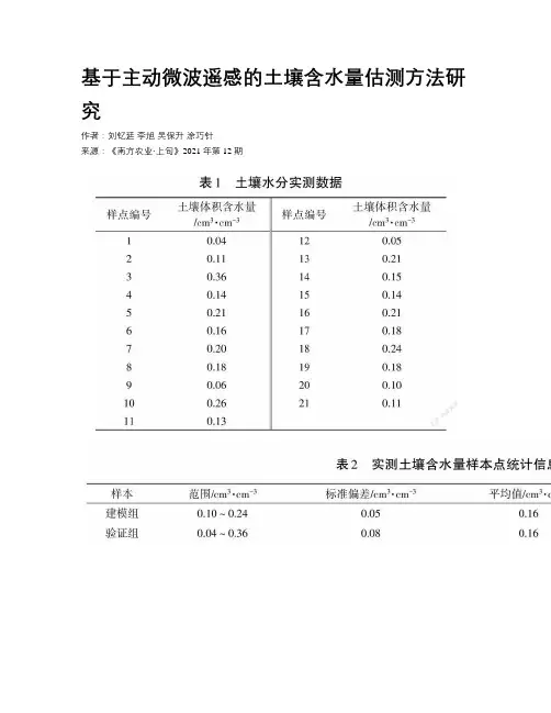
基于主动微波遥感的土壤含水量估测方法研究作者:刘钇廷李旭吴保升涂巧针来源:《南方农业·上旬》2021年第12期摘要農作物长势与土壤含水量密切相关,因此在农作物生长过程中能够及时准确地估测土壤水分十分重要。
研究主动微波遥感不同极化方式提取后向散射系数与地表土壤含水量之间的关系,建立土壤水分估测模型;通过分析不同地微波遥感信号基础上,建立土壤后向散射系数与土壤含水量的半经验模型,拟合VV极化、VH极化数据与土壤含水量实测数据。
实验结果表明:VV极化的决定系数R2=0.74,VH极化的决定系数R2=0.19,相较于VH极化,VV 极化的穿透性强、土壤水分含量变化更加敏感,适合用于土壤旱情监测,有助于把握最佳灌溉时机。
关键词土壤水分;主动微波遥感;后向散射系数;半经验模型;旱情监测中图分类号:S-03 文献标志码:A DOI:10.19415/ki.1673-890x.2021.34.035农作物生长离不开土壤水分,它是作物生存的重要物质基础之一。
土壤水分在地球上水循环运动中充当着十分重要的角色,也是水文、气象和农业相关研究中重要数据之一[1]。
当面对大面积区域的土壤水分测量时,传统测量方法会耗费大量人力、物力及时间。
因此,对土壤水分含量准确和高效的监测是农业水管理及农作物旱情预测的一个重要内容。
同时,在针对干旱区流域水文模型、农作物生长监测等方面问题也能起到一定作用。
利用微波遥感影像中提取数据监测土壤水分的技术到今天已经发展了40余年[2],由于微波估测土壤水分涉及地表粗糙度、植被覆盖度和土壤质地等多个方面的参数[3],而获取这些参数往往会受到一定的限制,如何充分利用微波数据源的各种辅助信息(如频率、极化方式等),降低对实地测量数据的依赖性,快速、便捷地获取大范围区域土壤水分分布情况是一直以来的研究热点。
搭载合成孔径雷达的主动微波遥感具有全天不间断工作、覆盖率高和信号穿透能力强的重要优势,使其成为土壤水分含量监测的有效手段之一,并且在各种土壤水分监测研究中应用十分广泛。
第40卷第6期2020年12月Vol.40No.6Dec.2020防灾减灾工程学报Journal of Disaster Prevention and Mitigation EngineeringDOI:10.13409/ki.jdpme.2020.06.016石灰改良土的土水特征曲线及其冻结特征曲线,王叶娇I,王有为I,靳奉雨I,马田田2"(1.上海大学土木工程系,上海200444;2.中国科学武汉岩土力学研究所,湖北武汉430071;3.岩土力学与工程国家重点实验室,湖北武汉430071)摘要:土水特征曲线反映了非饱和土的持水特性,与土体的水力特性及力学特性密切相关。
土的冻结特征曲线表示土体中液态水的势能与含水率之间的关系,也可以用来描述土体的持水特性。
以黄土为研究对象,利用低温恒温冷浴结合核磁共振系统(NMR)测得未处理黄土以及石灰改良土的冻结特征曲线,根据冻结温度降低法计算得出试验土样0°C时对应的土水特征曲线。
另外,采用滤纸法在0°C附近得到实测的土水特征曲线,将这两结果进行对比分析,并讨论了抽真空饱和过程对土样的土水特征曲线的影响。
通过滤纸法测得的土水特征曲线与非饱和土样的冻结特征曲线具有较好的一致性,两者之间存在差异很小。
土样在饱和状态下利用冻结温度降低法得到的孔隙水总势能#与质量含水率w关系曲线位于非饱和土样结果的下方,这可能是因为饱和土样在冻结过程中会发生冻胀现象,土样结构被破坏,孔隙增大,土样持水性能下降关键词:土水特征曲线;冻结特征曲线;非饱和土;核磁共振技术中图分类号:TU443文献标识码:A文章编号:1672^2132(2020)06-0967-07Soil-water Characteristic Curve and Freezing Characteristic Curve ofLime Improved SoilWANG Yejiao',WANG Youwei1,JIN Fengyu1.MA Tiantian2(1.Department of Civil Engineering,Shanghai University,Shanghai200444,China;2.State Key Laboratory of Geomechanics and Geotech n ical En g ineeri n g,Wuhan430071,China;3.Institute of Rock and Soil Mechanics,Chinese Academy of Sciences,Wuhan430071,China)Abstract:The soil-water characteristic curve(SWCC)indicates the water retention properties of unsaturated soil,which is strongly related to soil hydro-mechanical behavior.The freezing characteristic curve of the soil represents the relationship between the potential energy of the liquid water in the soil and the water content.It can also represent the water retention behavior of unsaturated soil.In this study,loess was selected as the research object.The freezing characteristic curves of untreated loess and lime-treated soil were obtained from a cryogenic thermostat cold bath and nuclear magnetic reso-nance(NMR)system,and then the soil-water characteristic curve at0°C was deduced by applying the freezing temperature reduction method.In addition,the measured soil-water characteristic curve was obtained by using the filter paper method at around0°C.The two results were compared and analyzed, and the influence of the vacuum saturation process on the soil-water characteristic curve of the soil *收稿日期:2020-05-05;修回日期:2020-09-11基金项目:国家自然科学基金项目(41702306)资助作者简介:王叶娇(1988-),女,讲师,博士。
土壤含水量的表达方法When it comes to expressing soil moisture content, there are a few different methods that are commonly used. The most common method is to use a measurement called volumetric soil moisture content, which is expressed as a percentage.谈到表达土壤含水量,通常有几种不同的方法。
最常见的方法是使用一种叫做体积土壤含水量的测量,它以百分比的形式表示。
This method measures the volume of water in a given volume of soil, and is often used in scientific research and agriculture to determine how much water is available to plants. Another method for expressing soil moisture content is using gravimetric moisture content, which measures the weight of water in a given weight of soil. 这种方法测量了一定体积土壤中的水量,并且通常在科学研究和农业中被用来确定植物可利用的水量。
另一种表达土壤含水量的方法是用重量法含水量,它测量了一定重量土壤中的水分重量。
This method is often used in soil science and geology to determine the physical properties of soil. Both methods have their strengthsand weaknesses, and the best method to use will depend on the specific application and the resources available.这种方法通常用于土壤科学和地质学来确定土壤的物理性质。
中国水土保持科学Science o£ Soil and Water Conservation第19卷第1期2021年2月Vol. 19 No. 1Feb.2021黄土高原不同林地土壤水分特征及影响因子通径分析胡波1,陈丽华5(1.北京林业大学水土保持学院,100083,北京;2.山西吉县森林生态系统国家野外科学观测研究站,042200,山西吉县)摘要:通过野外实测数据,研究土壤水分特征,用通径分析明确不同影响因子对土壤含水量的直接和间接作用。
在黄土高原研究区,分别在油松林、刺槐林和苹果林样地设立土壤水分动态观测点,用WaterScout SM 100 Sensor-6ft水分探头在2018年4—10月植被生长季观测不同土层的土壤体积含水量,同年8月,在不同林地分层进行土壤取样,测定土壤理化性质。
结果表明:1)观测林地土壤含水量之间存在显著差异(P<0. 05),苹果林土壤含水量总体 高于刺槐林和油松林;2)研究区不同林地土壤水季节变化趋于一致,总体呈先上升后下降趋势,生长季土壤总贮水量苹果(1 460. 38 mm) >油松(988. 02 mm) >刺槐(844. 66 mm);3) 土壤理化性质和土壤水分变化有显著的相关性,通过通径分析得出:影响最显著的因子为0. 050 -0. 002 mm 土壤颗粒含量,其决策系数为9. 825 ;密度对其有较大的间接作用;有机质和2. 000 - 0. 050 mm 土壤颗粒含量对土壤含水量有极显著的抑制作用,其决策系数分别为-2. 669和-5.645。
通径分析适用于土壤水分影响因子分析。
研究结果可为黄土高原地区林地树种选择及生态环境管理提参考。
关键词:土壤含水量;动态变化;通径分析;不同林地;黄土高原中图分类号:S152.7 文献标志码:A文章编号:2096-2673(2021)01 -0079-08DOI : 10.16843/j. sswc. 2021.01.010Characteristics of soil moisture and path analysis of influencing factors ondifferent forest lands on the Loess PlateauHU Bo 1, CHEN Lihua 1,2(1. School of Soil and Water Conservation , Beijing Forestry University , 100083, Beijing , China ;2. National Field Research Station of Forest Ecosystem in Jixian County , 042200, Jixian, Shanxi,China)Abstract : [ Background] Due to the influence of natural and human factors , soil erosion is a seriousproblem on the Loess Plateau. A large amount of vegetation has been planted on this plateau via varioussoil and water conservation measures and ecological restoration. At the same time, vegetation growth consumes a high amount of soil moisture ・ Soil-water deficit restricts vegetation growth and further affectsthe ecological environment improvement. The Caijiachuan watershed selected in this paper represents typical characteristics of the Loess Plateau. This study not only analyses the pattern of soil moisturechange and influencing factors , but also measures the applicability of the path analysis method ・[Methods ] In the study area of the Loess Plateau , we set up soil moisture dynamic observation points in the Pinus tabuliformis ( PT ) , Robinia pseudoacacia ( RP ) , and Malus domestica ( MD ) plotsrespectively , using the WaterScout SM 100 Sensor-6ft to observe the soil volumetric moisture content indifferent soil layers from April to October 2018. In the August of the same year, we sampled the undisturbed soil with a ring knife and obtained soil samples from different forest lands to determine the收稿日期:2020-06-13 修回日期:2020-11-30项目名称:国家重点研发项目“黄土残嫄沟壑区水土保持型景观优化与特色林产业技术及示范”(2016YFC0501704) 第一作者简介:胡波(1996—),女,硕士研究生。
基于Ts-EVI特征空间的土壤水分估算闫峰;王艳姣【摘要】温度-植被指数特征空间耦合了地表温度和植被信息,是当前实现土壤水分遥感估算和农业旱情监测的重要方法.采用EOS-MODIS地表温度Ts和增强型植被指数EVI数据,研究Ts-EVI三角形特征空间中干边、湿边方程参数的确定方法,分析比较了温度植被干旱指数TVDI对不同土壤深度水分状况的估算能力,为利用特征空间法实现土壤水分监测提供理论依据.研究表明:特征空间中干边和湿边的确定以最大拐点处为始点进行线性拟合的常规方法并不完善,根据像元的分布频率,以采用能同时保留最大量有效信息和较高拟合精度的端点逼近法获取参数的效果较好;基于Ts-EVI特征空间构建的TVDI可以较好地估算土壤表层10、20cm和50cm 土壤深度处土壤水分状况,其相关性均通过了α=0.001水平的t检验,但TVDI对表层土壤(20cm和10cm)水分的估算精度相对较高.【期刊名称】《生态学报》【年(卷),期】2009(029)009【总页数】8页(P4884-4891)【关键词】Ts;EVI;特征空间;土壤水分;河北【作者】闫峰;王艳姣【作者单位】中国林业科学研究院荒漠化研究所,北京100091;中国气象局国家气候中心,北京100081【正文语种】中文【中图分类】Q149;Q154.1利用传感器获得的地物波谱信息提取地表温度Ts和归一化植被指数NDVI等陆表参数进行估算土壤水分状况成为当前土壤水分和农业旱情监测的重要发展方向[1~5]。
在众多的土壤水分遥感信息模型中,温度植被干旱指数(temperature vegetation drought index, TVDI)耦合了Ts和NDVI信息,通过Ts-NDVI特征空间的变化特征分析土壤水分状况和实现农业旱情遥感监测得到了快速发展[6~9]。
在Ts-NDVI特征空间关系的研究中,Nemani等[10]认为二者表现为梯形的关系,Moran等[11]根据地表-大气温差和植被覆盖度的关系,通过构建的植被指数-温度梯形空间,进一步分析了作物缺水指数CWSI算法,使研究部分植被覆盖的地表状况时可以避开叶面温度的测量,具有重要的理论意义。
生物修复法处理新疆油田老化油泥试验李慧敏;张燕萍;肖丰浦【摘要】This paper takes the long-term piled up oily sludge in the northwest desert oil-field as the research objects. The activity of degradation of petroleum contaminants is strengthened by creating conditions conducive to microbial growth and reproduction. and the repairing effect is determined.Field test uses the experimental optimization of soil porosity (55%), soil moisture content(25%), bacteria agent additive amount 5%(mass fraction), N/P Ratio(10∶1) and additive amoun t of bio-surfactants5%. Oily sludge bioremediation ex-periment results show thatoil content of oily sludge is 0.11%~0.29% after six months, which reached the harmless emissions standards prescribed by the state(less than 0.3%).%以西北荒漠地区油田长期堆放的含油污泥为研究对象,通过创造有利于微生物生长繁殖的条件,强化其降解石油类污染物的活性,测定修复效果。
现场小试结果表明,采用试验优选的土壤孔隙度为55%、土壤含水率为25%、菌剂投加量为5%(质量分数)、氮磷比为10∶1、生物表面活性剂投加量为5%等参数,开展油泥生物修复试验,6个月后测得其含油量为0.11%~0.29%,达到了国家规定的无害化排放标准。
Agricultural and Forest Meteorology112(2002)67–85Transpiration response to soil moisture in pineand spruce trees in SwedenFredrik Lagergren∗,Anders LindrothDepartment of Physical Geography and Ecosystem Analysis,Lund University,Box118,SE-22100Lund,SwedenReceived28September2001;received in revised form9May2002;accepted14May2002AbstractVariation in transpiration and conductance between individual trees of Scots pine and Norway spruce was investigated in a mixed50-year-old stand in central Sweden.Daily transpiration rates were measured by the tissue heat balance method on five trees of each species during a dry,warm growing season.Daytime averages of sapflow,climatic variables and soil water content were used tofit an empirical model of tree conductance for each tree.Conductance per unit needle area was about twice as high in pine as in spruce,while equal-sized trees transpired similarly in both species.Conductance generally decreased more steeply with increasing vapour pressure deficit and increased faster with increasing light in pine than in spruce,although one individual spruce behaved more like the pines.Inclusion of a linear or exponential function for air temperature improved the model for pine,but of the spruces,only one tree showed a clear temperature dependency.The response to decreasing soil water content varied widely;the spruces tended to be more sensitive to drought than the pines.When the drought was at its worst,no sapflow could be detected in some of the trees.On average,the reduction in transpiration began when ca.80%of the extractable water in the rooting zone had been depleted.©2002Elsevier Science B.V.All rights reserved.Keywords:Stomatal conductance;Drought;Transpiration;Pinus sylvestris;Picea abies1.IntroductionTree transpiration is the major pathway for both water and energy leaving the forest ecosystem.Mea-surement of transpiration provides access to the canopy conductance of the forest,a key parameter in models of water-and carbon-exchange(Collins and Avissar,1994),since the water and carbonfluxes are strongly linked by their common passage through the stomata(Morén et al.,2001).∗Corresponding author.Tel.:+46-46-222-0000;fax:+46-46-222-4011.E-mail addresses:gergren@nateko.lu.se(gergren), anders.lindroth@nateko.lu.se(A.Lindroth).The scale at which the forest is studied answers dif-ferent questions in the context of exchanges of energy and matter(Jarvis,1995).Studies at shoot or branch level(e.g.Harley and Baldocchi,1995;Roberntz and Stockfors,1998),for instance,are particularly useful in the study of physiological processes;scaling-up to stand level from single shoots is intrinsically complex but can givefirm results(e.g.Baldocchi and Harley, 1995).Studies at tree level(e.g.Cermak et al.,1995; Granier et al.,1996)provide an average response of the mostly non-linear physiological processes,and are therefore,more useful for empirical modelling.Such studies are particularly useful for scaling-upfluxes for a certain stand or plot if a sufficient number of trees are measured(Cermak et al.,1995),and provide0168-1923/02/$–see front matter©2002Elsevier Science B.V.All rights reserved. PII:S0168-1923(02)00060-6gergren,A.Lindroth/Agricultural and Forest Meteorology112(2002)67–85answers about the variation within it.The ecosystem or landscape level(e.g.Tenhunen et al.,1998;Grelle et al.,1999)provides answers about net exchange and the variation between stands or regions.The sapflow technique(Swanson,1994)is very useful for obtaining the total water use of a single tree. Sapflow is commonly scaled up to stand level and con-sidered as representing transpiration.A problem with this approach is that,because of the capacitance of the trunk and branches,sapflow lags somewhat behind transpiration(Granier and Loustau,1994;Köstner et al.,1996).The lag is not constant over the course of the day,between days or between trees(Lundblad and Lindroth,2002;Phillips et al.,1997),even though in many approaches it is assumed to be constant; modelling the lag is consequently not a simple task. However,daily sapflow totals can often be assumed to equal the sum of transpiration,although under some conditions,e.g.after a dry period followed by some rainy days,this may not be true(Waring et al.,1979; Zweifel and Häsler,2001).Another drawback of a daily time step is that the processes which affect tran-spiration are non-linear,hence,any model would be truly empirical and should be used with caution out-side the range for which it was calibrated.The daily pattern of the variables can also vary between differ-ent days;this will affect conductance,even though the mean of the variables may be unchanged.Soil moisture is considered to be a critical parameter in many models of evaporation or surface energy par-titioning.Many models show large sensitivity to soil moisture,and general circulation models,which are used to predict future climate change,are no excep-tion(e.g.Viterbo and Beljaars,1995).Unfortunately, it is inherently difficult to establishfirm relationships between transpiration(or canopy conductance)and soil water content,mainly because of the large spa-tial variation in soil properties and soil moisture,but also because of transpiration’s strong dependence on other weather parameters.There are,however,several empirical studies of such relationships in whichfirm relationships have been established;e.g.for Scots pine by Rutter(1967),Sturm et al.(1996)and Irvine et al. (1998),for Norway spruce by Lu et al.(1995)and Lu et al.(1996),and for mixed stands of these species by Cienciala et al.(1998).As far as the present authors are aware,variation in individual response in a mixed stand has not previously been estimated and modelled.Evaluation of individual variation can increase our understanding of the response of the entire stand. The primary aim of this study was to quantify how tree conductance,and thus,the transpiration of indi-vidual trees in a mixed pine and spruce forest,depends on soil moisture.In order to do that it was also neces-sary to quantify the influence of weather conditions on the conductance of individual trees under non-limiting soil water conditions.Daily data from a growing sea-son with large variation in soil water content were used to estimate and model conductance and its de-pendence on weather parameters and soil moisture.2.Material and methods2.1.The standScots pine(Pinus sylvestris L.)and Norway spruce (Picea abies(L.)Karst)are dominant species in most of the Eurasian Taiga.Scots pine is a pioneer species that is well adapted to dry conditions.Norway spruce is a secondary species that is shade-tolerant and prefers wetter habitats that are not frequently disturbed.Mixed stands are,however,very common.The studied stand was located in the Norunda forest in central Sweden (60◦5 N,17◦29 E,altitude45m).The stand was ca. 50years old and was growing on a boulder-rich,sandy glacial till.The stand was naturally regenerated and was a mix of Scots pine(64%of the basal area(BA) at1.3m height),Norway spruce(33%)and deciduous trees(3%).A plot,60m×120m,was established in1997for studies of tree water relations,and the diameter of all trees on it was measured.The mean diameter was20cm,mean height was17m,BA was 29m2ha−1and there were872trees per hectare. 2.2.SapflowSapflow was measured by the tissue heat balance method(Cermak et al.,1973;Cermak et al.,1976; Cermak et al.,1982)with a P4.1sapflow meter(Eco-logical Measuring Systems,Bruno,Czech Republic). This is a method that has previously been proven to give reliable transpiration estimates in the studied for-est(Grelle et al.,1997;Cienciala et al.,1999)and the method was evaluated in Lundblad et al.(2001).The system usedfive electrodes inserted in parallel,andgergren,A.Lindroth/Agricultural and Forest Meteorology112(2002)67–8569 supplied with a constant power of1W,to heat a seg-ment of the stem.The temperature difference betweenthe heated and unheated part of the stem was measuredwith a thermo battery consisting of eight sensors.The measured temperature difference, T(K),iscorrelated to sapflow for the heated segment asQ w=Pc w T−kc w(kg s−1)(1)where P(W)is the heat input,c w the specific heat of water(4186.8J kg−1K−1)and k(W K−1)is the coef-ficient of heat loss from the heated segment,obtained under zero-flow conditions.Tree level sapflow,Q,was calculated by dividing Q w by the width of the heated segment(8cm)and multiplying by the circumference under bark at the measuring point.To record as much as possible of the variation in sapflow,both between trees and around the circumfer-ence of a tree,with the12sapflow channels available, the following set-up was used:the installations were made onfive pines andfive spruces in July1998(de-noted P1–5and S1–5).On each tree,two measuring points were installed,on the eastern and western side, respectively.On one pine and one spruce,both mea-suring points were continuously measured.Only one side of the other trees was connected on each mea-surement period.In1999,measurements were shifted from the east to the west side on16June and shifted back on5August.The two relationships,before and after the shifts,to the sapflow in the continuously mea-sured tree of the same species,was used to calculate a mean value based on measurements of both sides,as in Lundblad et al.(2001).There was a difference in sapflow between opposite sides,but the relationship was relatively stable(see Lundblad et al.,2001).In the present study,sapflow measurements from16April to 27October1999were used.In2000,the systems were installed in another sample of trees,sapflow from this year was used to validate thefinal model of the tran-spiration,this year sapflow was measured19May to 22October.No severe visual injuries were detected when the electrodes were removed in autumn1999. For the2days during which the measured side was shifted,sapflow was calculated as the mean fraction of theflow a few days before and after the shift,in the trees that was not shifted.Similarly,the missing days for P1,P3,P5,S1and S4on6–9July were replaced. For S5,the heating control malfunctioned from16June to6July and from6to11August.Data from these periods were replaced by data generated from the relationship with the remainder of the pines before and after the heating failure.2.3.Weather and soil moistureSoil water content(θ)at0–20and0–50cm depth, was measured with the TDR-technique(Topp et al., 1980)at eight positions located in a transect through the stand.This transect was not in the same direction as the sapflow transect,so it was not possible to link ‘local’soil moisture to the individual trees.A general formula for mineral soils was used to obtainθfrom the measurements.At each position,one pair of20cm rods and one pair of50cm rods were placed verti-cally.The signal was read manually about every tenth day during the growing season,by means of a Tek-tronix1502C cable tester(Tektronix Corp.,Beaverton, OR,USA).Additionally,θwas measured with two ThetaProbes(ML1,Delta-T Devices Inc.,Cambridge, UK),installed at10–15cm depth,which were read every minute with a Campbell CR10-datalogger and a Campbell AM32-multiplexer(Campbell Scientific Inc.,NE,USA).Data were stored as10min means. The dynamic information from the ThetaProbes was used to obtain interpolated daily values ofθ,based on the level of the mean of the TDR measurements. Fromθ,the relative extractable water(REW)(θREW) was calculated asθREW=θ−θmθFC−θm(2) whereθm is minimumθ(0.02for0–20cm and0.05 for0–50cm depth in the present study)andθFC isθat field capacity(0.30in the present study,both depths). Theθm was taken as the minimumθfound in the present study,and was in accordance with the wilting point found by Lundin et al.(1999)in an adjacent stand.TheθFC was taken as theθin the spring shortly after the groundwater table had fallen to the lower limit of the measured soil volume.Climatic data were taken from a tower ca.500m from the site and,for missing values,from a scaf-fold tower50m from the site(instrumentation is given in Table1).The data from the tower500m away were preferred,because the instruments in the scaffold tower were below the height of the tallest trees.gergren,A.Lindroth/Agricultural and Forest Meteorology112(2002)67–85 Table1Meteorological instrumentation in the Norunda tower and the scaf-fold towerQuantity InstrumentAir temperature Thermocouple(in situ,Ockelbo,Sweden)aHygrometer MP probe(RotronicInstruments Ltd.,Horley,UK)bRelative humidity Hygrometer MP probe(RotronicInstruments Ltd.,Horley,UK)a,bGlobal radiation Pyranometer CM-21(Kipp&Zonen,Delft,The Netherlands)aLI-190SZ quantum sensor(LI-CORInc.,Lincoln,NE,USA)bPrecipitation IS200W rain gauge(in situ,Ockelbo,Sweden)aData were recorded every minute with Campbell CR10-datalogger(Campbell Scientific Inc.,NE,USA)and stored as10min means.a Norunda tower.b Scaffold tower.2.4.Leaf area of the sapflow treesThe leaf area index(LAI)of the stand(L LAI2000)was estimated three times in1999with the LAI2000plant canopy analyser(LI-COR Inc.,Lincoln,NE).The measurements were corrected for foliage clump-ing by the factor1.65provided by the manufacturer,and averaged.The functions obtained from a detailed biomasssampling(Morén et al.,2000)were used tofind pro-jected leaf area(L tree)for all individual trees in thestand,with diameter as input.The L tree was correctedto sum up to the level of L LAI2000,because the sam-pled stand differed somewhat in age and the samplingwas done in a different year:L treecor=L tree L LAI2000AL tree(3)where A is the area of the plot(m2).Tree height and live crown length were measured both on the sapflow trees and on a sample of115 pines and85spruces.The needle mass according to Marklund(1988),was calculated from diameter at breast height,height and live crown length.For pine,the north co-ordinate,according to the Swedish co-ordinate system,was also included in the input pa-rameters.A relationship between diameter and needle mass was established for pine and spruce,respectively and was applied to all trees in the plot.Functions between needle mass and L treecor could then befitted for pine and spruce,respectively.The functions were used to obtain the projected leaf area of the sapflow trees from needle mass(in which tree height and live crown length were taken into account). The polynomial functions,on average,corresponded to specific leaf areas of7.3and4.5m2kg−1for pine and spruce,respectively which is close to the values in Morén et al.(2000).Thefinal leaf area of the sapflow trees was used to express sapflow per unit leaf area.The properties of the sapflow trees are summarised in Table2.2.5.Tree conductanceThe mean daytime value of temperature(T day(◦C)), vapour pressure deficit(D day(Pa))and global radi-ation(R day(W m−2))were calculated for the period when global radiation(R)>0.Daily sums of sapflow for each tree were calculated with no restriction in R, but were divided by the duration of R>0to obtain mean daytime transpiration per unit needle area(E day (g m−2s−1)).This was done because sapflow may be expected to lag behind transpiration,but transpiration will only occur when R>0.For pine and spruce,re-spectively mean values of E day,weighted by the leaf area were calculated,for which the conductance also was modelled.Tree conductance(g tday)was then cal-culated according to Monteith and Unsworth(1990): g tday=λE dayγρc p D day(4) whereλis the latent heat of vaporisation of wa-ter(2465J g−1),γthe psychrometer constant (65.5Pa K−1),ρthe density of the air(1225g m−3), and c p is the specific heat of air(1.01J g−1K−1).The use of this simplified equation for calculating conduc-tance is valid if the trees are well coupled to the at-mosphere,which can be assumed for conifers(Jarvis et al.,1976;Granier and Loustau,1994;Phillips and Oren,1998).The advantage of using a daily time step when modelling conductance is that the problem of the time-lag between sapflow and transpiration is overcome.The disadvantage is that Eq.(4)rightfully should be used on instantaneous values,but the errorgergren,A.Lindroth/Agricultural and Forest Meteorology112(2002)67–8571 Table2Dendrological properties of the pines(P1–5)and spruces(S1–5)in the present study and their distance to the centre of the nearest strip road(see Section4)P1P2P3P4P5S1S2S3S4S5 Diameter(cm)24.521.822.319.015.824.621.620.419.616.4 Height(m)17.016.816.715.416.919.016.617.216.516.0 Crown length(m)9.08.07.98.7 6.315.314.112.413.713.1 Leaf area(m2)62.747.448.944.323.5107.196.477.183.266.1 Needle mass(kg)8.81 6.35 6.60 5.86 2.4825.221.314.916.811.8 Distance to road(m)8.4 2.07.5 2.1 6.8 2.6 1.5 3.810.7 2.8is generally small,and thus acceptable,as described by Phillips and Oren(1998).To estimate the effect of soil moisture on tree conductance,it is necessary to analyse the influ-ence of weather conditions on conductance under non-limiting soil moisture conditions.Thus,the aim of the modelling described later was primarily to ob-tain a tool to‘normalise’conductances with respect to different weather parameters,i.e.not to obtain a general model of individual tree conductance.An empirical model of the calculated g tday wasfitted to vapour pressure deficit,radiation,temperature and soil moisture:g tday=g tmax f(D day)f(R day)f(T day)f(θ)(5) The modelling approach was stepwise,first g tmax and f(D day)was decided by using data when the other func-tions were close to1.Then f(R day)wasfitted when f(T day)and f(θ)were close to1,thereafter f(T day)when θwas not limiting,andfinally f(θ).The period18May to15June was used tofit the functions for D day and R day;this was a period with little variation in T day(mean15.2◦C;σ=2.2)and sufficient soil moisture.The function for T day wasfit-ted after the period from7July to27September had been excluded(during this period,θREW0–50cm was <0.30).Days with Penman potential evaporation(E p) (Penman,1948)less than1mm were also excluded as a small absolute measured error is likely to have a large effect when two small numbers are divided. Whenfitting the functions forθ,the period1June to15September was used,days with E p less than 1mm being excluded,as also days with D day above 2000Pa,because maximum D day during the period when f(D day)wasfitted was1355Pa.In total,there were11,2and12days,respectively,outside the range for which the functions for D day,R day and T day were fitted,from a total of189days for which thefinal model was applied.3.Results3.1.WeatherThe winter and early spring of1999were wet. Precipitation from December to April was270mm, i.e.64%more than for the normal period1960–1990 (Uppsala Weather Station,30km south).The growing season began with high soil water content(θ)and with the ground water table at or close to the soil surface at many points.May,June and August had precip-itation and temperature close to the normal,while July and September were warmer than normal,by1.9 and3.2◦C,respectively(Fig.1a).In July,only about one-third of the normal precipitation fell,and thefirst half of September was also very dry.This depleted the soil water,andθ0–50cm decreased to minimum values<6%on4August and15September(Fig.1b). After some rainy days at the end of June,at the end of July and at the beginning of August,θrecovered temporarily.In the middle of July,and at the turn of the month to August,there were some days with very warm and dry conditions.The mean daytime vapour pressure deficit(D day)then had a maximum value of ca.2400Pa(Fig.1c).3.2.SapflowThe decreasingθhad a high impact on the sapflow rate.In spite of high demand,i.e.high vapour pressure deficit and global radiation(Fig.1c)in middle of July,gergren,A.Lindroth/Agricultural and Forest Meteorology112(2002)67–85Fig.1.Environmental conditions and sapflow for the1999season.(a)Mean daytime temperature,T day(thin line)and accumulated monthly precipitation(bold line).In April,a manual rain gauge was emptied a few times and only a total for this month is presented.(b)Soil water content at0–20cm(normal line)and0–50cm(bold line)depth.The points are means from manual reading of eight positions with TDR rods and the lines are calculated from the dynamics of continuously measured ThetaProbes.(c)Mean daytime vapour pressure deficit, D day(bold line)and mean daytime global radiation,R day(thin line).(d)Seven-day running means of sapflow for the pines P1(thin line), P2(normal line)and P4(bold line).(e)Seven-day running means of sapflow for the spruces S1(thin line),S2(normal line)and S3(bold line).The presented trees were selected to represent the range in soil moisture response.F .Lagergren,A.Lindroth /Agricultural and Forest Meteorology 112(2002)67–8573at the beginning of August and the end of September,sapflow decreased dramatically (Fig.1d and e ).At the beginning of July,the first trees began to respond to the decreasing θ,while others maintained transpiration a few weeks longer.This individual behaviour can be demonstrated by comparing the relationship in sapflow rates between trees at the beginning of June,when soil water content was high,with a period in Septem-ber,when soil water content was low and decreasing (Fig.2).The three selected pines did not differby Fig.2.Sapflow and environmental conditions for 2days in June and 6days in September 1999(note that the x -axis is not continuous).(a)Sapflow for the pines P1(thin line),P2(normal line)and P4(bold line).(b)Sapflow for the spruces S1(thin line),S2(normal line)and S3(bold line).(c)Soil water content at 0–50cm.(d)Global radiation (normal line)and vapour pressure deficit (bold line).The presented trees were selected to represent the range in soil moisture response.more than about 20%at most in June,whereas the difference in mid-September was 15orders of mag-nitude between the tree with the highest maintained sapflow rate,and that which was least able to tran-spire (Fig.2a ).It may also be noted that the tree with the highest sapflow rate in June decreased most in September,while the tree with the lowest rate in June maintained its flow rate best.The picture was simi-lar for the spruces,but here all trees decreased their sapflow rates to almost zero in mid-September.74F .Lagergren,A.Lindroth /Agricultural and Forest Meteorology 112(2002)67–853.3.Tree conductanceThe period 18May to 15June was selected to fit the functions f (D day )and f (R day ),because soil mois-ture was high at the same time as there was a large variation in vapour pressure deficit and global radia-tion.Tree conductance showed the characteristic be-haviour for conifers,i.e.decreasing conductance with increasing D day ,with a large scatter for low D day and increasing conductance with increasing R day (Fig.3).The pines showed a stronger response to high D day than the spruces.The g tday increased with increasing R day in a logarithmic fashion.For the pines,there was a tendency towards decreasing g tday at the high-est radiation levels,which was caused by the steep response to D day .The correlation between D day and R day was high,r 2=0.65.As the first step,the dependence on D day was con-sidered by applying boundary-line analysis (Webb,1972;Martin et al.,1997).Lines were fitted to theup-Fig.3.Tree conductance,based on sapflow per unit projected needle area,dependence on daytime vapour pressure deficit (D day )and daytime radiation (R day )for the period 18May to 15June 1999.(a)Dependence on (D day )for pines,P1(×),P2(+),P3(᭺),P4( )and P5(᭛),the lines are fitted through boundary-line analysis (see text).(b)Dependence on D day for spruces,S1(×),S2(+),S3(᭺),S4( )and S5(᭛).(c)The pines’dependence on R day (symbols as in (a)).(d)The spruces’dependence on R day (symbols as in (b)).per right part of Fig.3a and b ,where no limitation due to low radiation could be expected.Although the relationships seemed linear for the pines,exponential functions of the form:g tday =g tmax exp (−aD day )(6)were used,where g tmax and a are fitted parameters whose values are given in Table 3;g tmax is a hy-pothetical conductance at zero D day and saturated radiation,which varied between 5.9and 14.3mm s −1for the pines and between 1.3and 2.6for the spruces.The parameter a was ca.0.002for the pines and 0.001for the spruces.Exponential functions were preferred,to make extrapolation possible,as this is the known common behaviour (e.g.Stewart,1988).As the next step,the dependence on global radiation was considered.The quotient between measured con-ductance (Eq.(4))and g tmax ×f (D day )was regarded as a function of R day (Fig.4).The relationships weregergren,A.Lindroth/Agricultural and Forest Meteorology112(2002)67–8575 Table3Parameters for the conductance,g tday,functions of vapour pressure deficit,D day,and radiation,R day(g tday=g tmax exp(−aD day)(b ln R day−c)),for the pines P1–5,the spruces S1–5and for a weighted average for respective speciesP1P2P3P4P5S1S2S3S4S5Pine Spruce g tmax(mm s−1)11.0510.4314.31 5.917.12 1.55 1.31 2.35 2.60 1.7610.44 1.48a×103 2.15 2.12 2.44 1.46 2.04 1.29 1.080.920.99 1.55 2.120.92b0.5630.5550.5730.5820.5760.4580.4970.4570.4710.6150.5780.470 c 2.51 2.49 2.60 2.50 2.57 1.84 2.21 1.87 1.93 2.79 2.59 1.91Fig.4.The ratio of measured conductance(g tday)to conductance modelled using vapour pressure deficit(g tmax f(D day))plotted against global radiation;the lines are logarithmic regressions and data are from18May to15June1999.(a)Pines P1(×),P2(+),P3(᭺),P4 ( )and P5(᭛).(b)Spruces S1(×),S2(+),S3(᭺),S4( )and S5(᭛).76F .Lagergren,A.Lindroth /Agricultural and Forest Meteorology 112(2002)67–85best described by logarithmic functions:f (R day )=b ln R day −c(7)where b and c are parameters.When the functions de-livered negative values (if b ln R day <c ),the function was set to zero.This point,below which no transpira-tion occurred during the day according to the model,accorded to R day values between 60and 95W m −2.The values of the parameters,b and c ,are listed in Table 3.For the mean pine,b and c were 0.58and 2.6,respectively and for spruce 0.47and 1.9,respec-tively.S5deviated somewhat from the other spruces,by exhibiting values more like those of the pines.Finally,the effect of air temperature on the conduc-tances was dealt with in the following manner.For the pines,there was a strong relationship between the quotient between measured conductance (Eq.(4))and conductance modelled with R day ,D day and mean day-time air temperature (Fig.5).For four of the trees,the relationship was best described by an exponential function:f 1(T day )=k exp (lT day )(8)For one tree,the relationship was linear:f 2(T day )=mT day(9)The quotient showed a clear linear response to tem-perature for one of the spruces only,for the rest of the spruces,there was no relationship,i.e.f 3(T day )=1(10)The parameter values (k ,l and m )and the function used for each tree are given in Table 4.Accordingly,it was now possible to assess the ef-fect of soil moisture on tree conductance.The quotient between measured conductance (Eq.(4))and conduc-tance modelled with radiance,vapour pressure deficit,and temperature,showed a strong dependence on theTable 4The function used for temperature,T day ,dependence of the conductance and the derived parameters (f 1(T day )=k exp (lT day ),f 2(T day )=mT day ,f 3(T day )=1),for the pines P1–5,the spruces S1–5and for a weighted average for respective speciesP1P2P3P4P5S1S2S3S4S5Pine Spruce f (T day )111212333313k 0.1600.1700.123–0.222–––––0.171–l 0.1140.1130.130–0.095–––––0.110–m–––0.063–0.066––––––relative amount of extractable water,θREW (Fig.6).Linear functions up to a threshold value (x )were used to describe the relationships:f (θ)=θREWx,x <θREW(11)f (θ)=1,x =θREW(12)To obtain x ,Eqs.(11)and (12)were combined to one equation (Eq.(13))which was solved by the ‘nlin procedure’in SAS statistical software (version 6.12,SAS Institute,Cary,NC):f (θ)= θREW x |x −θREW |(x −θREW )+1+|θREW −x |(θREW −x)+1×0.5(13)The threshold value (x )was derived for both θREW 0–20cm and θREW 0–50cm ;the values of x are listed in Table 5.The variation in x was large,be-tween 0.04and 0.37θREW 0–50cm for the pines and between 0.18and 0.39for the spruces.The slope and the r 2values for the relationship be-tween measured conductance and conductance mod-elled with all functions in Eq.(5),are given in Table 6.The conductance in the early spring and late autumn was difficult to explain by the model for some of the spruces,for which reason,the relationships restricted to the period 1May to 30September are also given.For the pines,there was little difference between the model fitted to θREW 0–20cm or θREW 0–50cm ;it ex-plained 46–74%of the variation,and underestimated conductance by 0–14%.For the spruces,when the spring and autumn period were excluded,the model was improved by 1–6%if θREW 0–20cm was used in-stead of θREW 0–50cm ;r 2was between 0.59and 0.80,and the slope was between 0.94and 1.0when the re-stricted period and θREW 0–20cm were used.。