W and Z transverse momentum distributions resummation in qT-space
- 格式:pdf
- 大小:339.94 KB
- 文档页数:32

高中物理英语词汇机械运mechanical motion [mi'k?nik?l] ['m?u??n]力学mechanics [m?'k?n?ks]质点mass point [m?s] [p?int]参考系reference frame ['refr?ns] [freim]坐标系coordinate system [k?u'?:dineit] ['sist?m]路程path[pɑ:θ]位移displacement[d?s'ple?sm?nt]矢量vector['vekt?]标量scalar['skeil?]速度velocity[vi'l?siti]平均速度average velocity['?v?rid?] [vi'l?siti瞬时速度instantaneous velocity[,?nst?n'teinj?s]速率speed[spi:d]v-t 图象v-t graph[ɡrɑ:f]加速度acceleration [?k,sel?'re???n]普朗克Planck匀变速直线运动uniform variable rectilinear motion['ju:nif?:m] ['v??ri?bl] [,rekti'lini?]初速度initial velocity[i'ni??l] [vi'l?siti]自由落体运动free-fall motion自由落体加速free-fall acceleration[?k,sel?'re???n]重力加速度gravitational acceleration[,ɡr?vi'tei?n?l]伽利略Galileo Galilei力force[f?:s]牛顿Newton['nju:tn]重力gravity['ɡr?viti]重心center of gravity['sent?]万有引力gravitation[,gr?v?'te???n]电磁相互electromagnetic interaction[?,lektr??m?g'net?k]强相互作用strong interaction[,?nt?r'?k??n]弱相互作用weak interaction形变deformation[,di:f?:'me???n,]弹性形变elastic deformation[i'l?stik] [,di:f?:'me???n,]弹性限度elastic limit[i'l?stik] ['limit]弹力elastic force[i'l?stik] [f?:s]劲度系数coefficient of stiffness[,k???'f???nt] ['st?fn?s]胡克定律Hooke law[l?:]摩擦力friction force['frik??n]静摩擦力static frictional force['st?tik] ['frik??n]滑动摩擦力sliding frictional force['slaidi?]动摩擦因数dynamic friction factor[dai'n?mik]合力resultant force[ri'z?lt?nt]分力component force[k?m'p?un?nt]力的合成composition of forces[,k?mp?'zi??n]平行四边形定则parallelogram rule[,p?r?'lel?,gr?m]共点力concurrent forces[k?n'k?:r?nt,]力的分解resolution of force[,rez?'lu:??n]三角形定则triangular rule[tra?'??gj?l?] [ru:l]运动学kinematics[kini'm?tiks]动力学dynamics[dai'n?miks]牛顿第一定律Newton first law['nju:tn] [l?:]惯性inertia [i'n?:?j?]惯性定律law of inertia[i'n?:?j?]质量mass[m?s]惯性系inertial system['sist?m]牛顿第二定律Newton second law单位制system of units国际单位制Le Systeme International Unites SI[,?nt?'n???n?l]作用力action['?k??n]反作用力reaction[ri'?k??n]牛顿第三定律Newton third law超重overweight[,??v?'we?t]失重weightlessness['we?tl?s]误差error['er?]偶然误差accidental error[,?ksi'dentl]系统误差systematic error [,sist?'m?tik]绝对误差absolute error['?bs?lu:t]相对误差relative error['rel?tiv]亚里士多德Aristotle曲线运动curvilinear motion[k?:vi'lini?]基尔霍夫Kirchhoff切线tangent['t?nd??nt]抛体运动projectile motion[pr?'d?ekt?l,]抛物线parabola[p?'r?b?l?]线速度linear velocity['lini?]匀速圆周运动uniform circular motion['ju:nif?:m] ['s?:kjul?]角速度angular velocity['??gj?l?]弧度radian['reidj?n]周期period['pi?ri?d]向心加速度centripetal acceleration[sen'tr?p?tl]向心力centripetal force[sen'tr?p?tl]开普勒Kepler引力常量gravitational constant[,ɡr?vi'tei?n?l]['k?nst?nt]万有引力定律law of universal gravitation[,ju:ni'v?:s?l]第一宇宙速度first cosmic velocity['k?zmik]第二宇宙速度second cosmic velocity第三宇宙速度third cosmic velocity黑洞black hole能力energy['en?d?i]势能potential energy[p?'ten??l]动能kinetic energy[k?'net?k, ka?-]功work[w?:k]焦耳joule[d?u:l]功率power['pau?]瓦特watt['pau?]重力势能gravitational potentialenergy[,ɡr?vi'tei?n?l][p?'ten??l]弹性势能elastic potential energy[i'l?stik] [p?'ten??l]动能定理theorem of kinetic energy['θi:?r?m]机械能mechanical energy[mi'k?nik?l] [k?'net?k]机械能守恒定律law of conservation of mechanical energy[,k?ns?'vei??n] [mi'k?nik?l]能量守恒定律law of energy conservation[,k?ns?'vei??n]亥姆霍兹Helmholtz['helmh?ults]力 force拉力 traction['tr?k??n]力矩 torque[t?:k]动量 momentum[m?u'ment?m]角动量 angular momentum['??gj?l?]振动 vibration[va?'bre???n]振幅 amplitude['?mpl?,tu:d, -,tju:d]波 wave[weiv]驻波 standing wave['st?nd??]震荡 oscillation[,?s?'le???n]相干波 coherent wave[k?u'hi?r?nt]干涉 interference[,?nt?'fi?r?ns]衍射 diffraction[di'fr?k??n]轨道 obital大小 magnatitude方向 direction[di'rek??n]水平 horizental竖直 vertical['v?:tik?l]相互垂直 perpendicular[,p?:p?n'd?kj?l?]坐标 coordinate[k?u'?:dineit]直角坐标系 cersian coordinate system极坐标系 polar coordinate system['p?ul?]弹簧 spring[spri?]球体 sphere[sfi?]环 loop[lu:p]盘型 disc圆柱形 cylinder['silind?]械振动 mechanical vibration [va?'bre???n]简谐振动 simple harmonic oscillation [hɑ:'m?nik]振幅 amplitude ['?mpl?,tu:d, -,tju:d]频率 frequency ['fri:kw?nsi]赫兹 hertz [h?:ts]单摆 simple pendulum ['pendjul?m]受迫振动 forced vibration共振 resonance ['rez?n?ns]机械波 mechanical wave介质 medium ['mi:dj?m]横波 transverse wave [tr?ns'v?:s]纵波 longitudinal wave [l?nd?i'tju:dinl]波长 wavelength ['we?v,le?kθ]超声波 supersonic wave [,sju:p?'s?nik]。

语义分析的一些方法语义分析的一些方法(上篇)•5040语义分析,本文指运用各种机器学习方法,挖掘与学习文本、图片等的深层次概念。
wikipedia上的解释:In machine learning, semantic analysis of a corpus is the task of building structures that approximate concepts from a large set of documents(or images)。
工作这几年,陆陆续续实践过一些项目,有搜索广告,社交广告,微博广告,品牌广告,内容广告等。
要使我们广告平台效益最大化,首先需要理解用户,Context(将展示广告的上下文)和广告,才能将最合适的广告展示给用户。
而这其中,就离不开对用户,对上下文,对广告的语义分析,由此催生了一些子项目,例如文本语义分析,图片语义理解,语义索引,短串语义关联,用户广告语义匹配等。
接下来我将写一写我所认识的语义分析的一些方法,虽说我们在做的时候,效果导向居多,方法理论理解也许并不深入,不过权当个人知识点总结,有任何不当之处请指正,谢谢。
本文主要由以下四部分组成:文本基本处理,文本语义分析,图片语义分析,语义分析小结。
先讲述文本处理的基本方法,这构成了语义分析的基础。
接着分文本和图片两节讲述各自语义分析的一些方法,值得注意的是,虽说分为两节,但文本和图片在语义分析方法上有很多共通与关联。
最后我们简单介绍下语义分析在广点通“用户广告匹配”上的应用,并展望一下未来的语义分析方法。
1 文本基本处理在讲文本语义分析之前,我们先说下文本基本处理,因为它构成了语义分析的基础。
而文本处理有很多方面,考虑到本文主题,这里只介绍中文分词以及Term Weighting。
1.1 中文分词拿到一段文本后,通常情况下,首先要做分词。
分词的方法一般有如下几种:•基于字符串匹配的分词方法。
此方法按照不同的扫描方式,逐个查找词库进行分词。

发电厂:power plant组态:configuration补偿电缆:building out cable电缆敷设:cable laying热继电器:thermorelay配电:distribution就地:on-site电磁阀:electro valve铠装电缆:armored cable校验:checkout冗余:redundancy熔断器:fusible cutout固态电路:solid-state circuit电缆桥架:cable crane span structure分散控制系统DCS:Distributed Control System 数据采集系统(DAS):Data Acquisition System 模拟量控制系统(MCS):Mimesis Control System 顺序控制系统(SCS):Sequences Control System 操作员站(OS):operator station工程师站(ES): engineer station盘、箱、柜、台:panel、box、cabinet、board 联锁:interlock可编程控制器(PLC):programmable logic controller施工图:execution drawing竣工图:completion drawing防爆:explosion proof变送器:transmitter变频器:frequency converter双金属温度计:bimetallic thermometer热电偶:thermocouple热电阻(RTD): Resistive Thermal Detector 保护套管:adapter pipe差压:differential pressure仪表盘:instrument panel电磁流量计:electromagnetism flowmeter密度计:densimeter电磁波:electromagnetic wave排放:sluice锅炉:boiler进线:incoming line母线:bus line(工作)变压器:(main)transformer直流:direct current手轮:hand wheel控制回路:control circuit减压阀:reducing valve二线制(三线制):two wire system(three wire system)电磁制动:electromagnetic braking人机界面:human machine interface机组:machine shop端子排:group terminal block接地:connect to earth(earthing)屏蔽:screen(shield)自诊断:self diagnostics电池失效:battery’s out of work高(低)电平:high(low)level耦合:complex coupling电除尘器:electrostatic dust catcher闭锁:lock-out(closure)历史数据的存储和检索(HSR): Saving and Retrieval of the History data消防:fire protection电磁干扰:electromagnet interference循环冗余校验(CRC): cyclic redundancy checkout烟气脱硫: flue gas desulfurization脱硫岛:desulfurizing island环氧树脂:Epoxy resin化学耗氧量:chemic consumption of oxygen电导率:Conductance ratio破碎机:Crushing machine湿式球磨机: Wet ball crusher阻燃聚丙稀:Flame retarding polypropylene 水力漩流器:hydrocyclone真空皮带脱水机:Vacuum belt filter鳞片树脂内衬flake resinous liner硫化: sulfidation氧化风机:Oxidizing fan真空泵: Vacuum pump6KV 公用配电屏 6kv station board6KV配电屏 6kv unit boardZ型拉筋 zig-zag rod安培 A: ampere氨 ammonia按钮 push button按钮 pushbutton按钮触点 push contact按时间顺序的 chronological半导体 semiconductor半径的、辐射状的 radial饱和水 saturated water保护和跳闸 protection and trip报警器 annunciator备用 back-up备用 provision备用 reserve比特、位 bit闭环 closed loop避雷器 surge diverter变电站 substation变送器 converter变送器 transmitter变压器 transformer并网 synchronization并行接口 parallel interface波特率 baud rate不导电的、绝缘的 dielectric不断电电源 Uninterruptible power supply(UPS) 不连续的 discrete采样器 pick-ups操作机构 mechanism操作台 the front pedestal侧墙 side wall测试仪表 instrument叉型叶根 multifork root长久的 permanent长期停机 prolong outage厂环 plant-loop厂用变 unit transformer超导体 superconductor超高压 EHV :extra-high voltage成组的、成批的 batch持续时间 duration尺寸 dimension充电器 charger冲动式汽轮机 impulse turbine冲击耐受电压 impulse withstand voltage除盐水 demineralized water除氧器 deaeratorD.A传送、运输 transport串(行接)口 serial interface串行存取 serial access吹灰器 sootblower吹扫 blow/purge垂直的 Vertical磁场作用 the action of a magnetic field磁导率 permeability次烟煤 subbituminous枞树形叶根 fir-tree root错误检验和恢复 error checking and recovery 错误指示器 error detector大规模集成电路 large scale integrate circuit 大修 overhaul单向流动 single-flow氮 nitrogen导纳 conductance导体 conductor导叶 Vane低压厂用变 sub-distribution transformer低压缸 low pressure cylinder/casing(LP)点火 light/ignite点火器 igniter电厂 power plant电磁 Solenoid电导率 conductibility电动操纵的 motor-operated电动机控制中心 MMC: motor control center电动机启动装置 motor starter电动液压的 electro-hydraulic电感电流 inductive current电抗 reactance电缆 cable电流互感器 CT :current transformer电气设备 electrical equipment/apparatus电容 capacitance电容电流 capacitive current电容器 capacitor电枢 armature电网 grid电网 network电涡流式检测器eddy current proximity detector电压互感器PT: potential /voltage transformer电压转换器 electric pressure converter电压自由触点 volt free contact电源 power supplies电站(水) power station电阻 resistance吊耳 lug调节、调制 Modulation调速器 governor调制解调 modulation-demodulation顶点 apex顶棚管 roof tube定位 orientation定子 stator定子机座 stator frame动稳定 dynamic stability动叶片 moving blades/ blading独立存在的 autonomous独立的 free standing端子、接线柱 instrument terminal端子箱、出线盒 terminal box断路器 circuit breaker锻造 casting对称度 symmetry对流烟道 convection pass多功能处理器 Multi Function Process(MFP)多项式 order polynomial额定负荷 ECR:economic continuous rating二极管 diode二进制单元 binary cell二进制的 binary二进制计数器 binary counter发电机 generator发光二极管 LED反动式汽轮机 reaction turbine反馈 feed back反相显示 reverse video沸腾 boil分辨率 resolution分层(级)的 hierarchical分隔墙 division wall分接头 tap分接头绕组 tapping winding分散控制系统 distribute control system(DCS) 分析基 air dry分压器 diverter粉状燃料 ground coal /pulverized fuel风道 duct风箱 wind box伏特 V: volt符号字符 character幅度 amplitude辅助的 auxiliary负压燃烧 suction firing附属部分 annex复制的、备用的 duplicate副励磁机 pilot exciter改造 alteration干式电缆 dry -core cable干燥基 dry感抗 inductance感应的 inductive高级的、先进的 sophisticated高压缸 high pressure cylinder/casing(HP)隔板 diaphragm 隔间 bay隔离开关 disconnecter给煤机 coal feeder给煤机转速信号 feeder speed跟随 shadow工程单位 engineering unit工业分析 proximate analysis工业锅炉 industrial boiler公差 tolerance公用锅炉 utility boiler公用系统 common service system鼓风机 forced draft fan固定碳 fixed carbon关合电流 making current管板 tube sheet管道 pipe管排 tube bundle管形的 tubular管子 tube管座 tube seat光电 photo-electric光洁度 finish硅 silicon锅炉 boiler/steam generator锅炉自动控制 Automatic Boiler Controls 过程处理单元 Process Control Unit (PCU) 过冷水 subcooled water过量空气 excess air过热器 superheater毫伏 millivolt褐煤 brown coal/lignite横向的 transverse后端、末端 rear end户内的 indoor滑环 Slipping化石燃料 fossil fuel还原气氛 reducing condition/atmosphere 环状的 annular灰分 ash挥发分 volatile机柜 cubical机座 frame级间漏汽 interstage leakage集控室 central control room (CCR)记录、日志 log架空的 overhead架空输电线 overhead transmission line 间隙 clearance兼容性、相容性 compatibility监测 monitoring监督管理 supervise监控方式 monitor mode监控器 monitor/monitor unit减温器 Attemperator检验 calibration交流电 alternating current接口 interface节点 node截止阀 stop/emergency valve紧急的应力 emergency stress经由 Via静叶片 stationary blades/ blading绝缘 galvanic isolation绝缘子 insulator开断 interruption开断电流 breaking current开关 switcher开关柜 switch cabinet开关柜 Switchgear开关组 switch block开环 open loop开环 open-cycle可编程逻辑控制器programmable logic controller(PLC)可编程只读存储器programmable read only memory(PROM)可靠性 reliability可燃基 dry and ash free可视通讯 visual communication空气断路器 air circuit breaker空气绝缘的 air-insulated空气预热器 air preheater控制按钮 control button(knob)控制精度 control accuracy控制屏 the operations panel控制器 controller控制室 the control room控制台 control console(desk)控制线圈 search coil控制仪表系统control and instrumentation(C&I)控制作用 control action浪涌 surge冷端补偿 cold junction compensation励磁 excite励磁机 exciter 例外报告 exception report联氨 hydrazine联锁 interlock联锁触点 interlocking contact联锁开关系统 interlocking switch system联锁信号 interlocking signal联箱 header联轴器 coupling裂纹 crack/cracking临界压力 critical pressure令牌 token流量 flow rate流量计 flow meter硫 sulfur/sulphur六氟化硫 sulphur hexa fluoride露点 the dew point temperature炉膛 furnace螺钉 screw毛胚 blank毛胚 roll媒介、介质 medium煤 coal煤粉燃烧器 PF burner/pulverized fuel burner 密度热电阻 density RTD灭弧 quench模块 workhouse模拟量 analogue模拟图 Mimic模拟子模块 ASM模数转换 Analogue to Digital conversion膜式壁 membrane panel/wall磨煤机 pulverizer/mill母线 busbar/bus内部的 internally内缸 inner casing能共存的、兼容的 compatible能量管接头 energy stud/stub凝结 condensate欧姆 ohm排污管 blowdown pipe盘车装置 turning gear配电 distribution配电盘、屏、板 panel膨胀 expansion疲劳、软化 fatigue偏心度 eccentricity平方根 square root平面 plane平直度 alignment齐纳二极管 Zener diode启备变 start up/standby transformer /启动 start up启动控制阀 pneumatic pilot valve气态 gaseous汽包 steam drum汽封片 gland segment/packing汽缸 cylinder汽机监视仪表turbine supervisory instrument(TIS)汽轮机 turbine汽泡户外的 bubble outdoor汽水混合物 steam-water -mixture千伏 kilo-volt前后墙 front/rear wall /强迫循环 forced/pumped circulation切除、切断、脱扣 trip氢 hydrogen求出的数量 evaluate全功能组件 complete functional set全貌、总的看法 overview燃料烟道 fuel /flue /燃烧器 burner扰动 intervetion/disturbing/bump绕组 winding热电厂 thermal power plant热电偶 thermocouple热电偶 thermocouple热工仪表 thermodynamic instrumentation热量加热 heat /热效率 thermal efficiency热应力分析 thermal stress analysis容量 capacity熔断 blow熔断器 fuse冗余测试 redundancy testing冗余的 redundancy冗余位 redundancy bit蠕变 creep散热片 cooling fin上半部 the top half蛇形管 serpentine tube设备、工具 facility省煤器 economizer湿蒸汽 wet-steam十二进制 duodecimal十进制的 decimal 十六进制 hexadecimal石油 oil使分流 shunt使完整 integration视频 visual frequency视像扫描器 visual scanner试运行 Commission试运行 commissioning operation疏水 Drain疏水管 drain pipe树脂浇注变压器 cast resin transformer 数字显示 digit display数字信号 digit signal双层缸结构 double shell structure双列端子排 two-tier terminals双向流动 double-flow双重的固态 dual solid水 water水电站 hydraulic power plant水分 moisture水冷壁 furnace tube水平的 horizontal水平接合面 the horizontal joint水位 water level水位计 gauge glass水压实验 hydrostatic test水蒸气 steam/water vapor酸洗 acid cleaning算法 algorithms榫头 tenon探针 probe碳 carbon天然气 natural gas条形 bar条形图 bargraph铁素体 mill铁芯 core停机 shut down停运 outage通道、信道 channel同类的 peer推力轴承 thrust bearing瓦特 W: watt外缸 outer casing网络接口子模块 INNIS微型调速器 microgovernor围带 shroud/shrouding温度 temperature文件缓冲器 archive buffer稳定性 stabilization稳态 steady-state无烟煤 anthracite物品、元件 item误差率 error rate误动作 malfunction熄灭、灭火 extinction铣制 forging系统 scheme: system下半部 the bottom half线圈 coil线性差动变压器 linear variable differential transformer (LVDT)线性化 linearization相变 phase change相互 interconnection相互隔离 isolate相同的 Uniform :the same消耗 consumption销钉 dowel协调的 harmonious协调控制系统coordination control system(CCS)信号调节 signal conditioning星型 palm terminal星型连接 connected in star形凹槽 notch V压力 pressure压力表 pressure meter烟道 flue烟煤 bituminous烟气 flue gas烟气热风器 gas air header氧 oxygen氧化气氛 oxidized condition/atmosphere叶顶 tip叶根 root叶轮 impeller/wheel/disk液态 liquid一氧化碳 monoxide一组 suite仪表量程 instrument range仪表灵敏度 instrument sensitivity仪表校正 instrument correction仪器盘 instrument board仪器仪表板 facia/fascia引风机 induced draft fan 应用基 as received永久磁铁 permanent magnet油浸式电缆 oiled-cable油枕 expansion tank有载调压的 load tap-changing元素分析 ultimate analysis原煤斗 coal bunker圆形的 circular圆柱形的 cylindrical圆锥形的 conical运行操作 operation /运行工况 operation condition再热器 reheater兆伏安 MVA: mega volt-ampere真空断路器 vacuum contactor振动 Vibration蒸发 evaporate蒸汽热风器 steam air header整流 rectify正压燃烧 pressure firing支持轴承 journal bearing执行机构 actuator直观显示元件 visual display unit (VDU)直观显示终端visual (inquiry)display terminal直流电阻 D.C. resistance质量 quality中心度、同心度 concentricity中心线 centerline中性点 neutral point中压缸intermediate pressure cylinder/casing(IP)终端、端子 terminal终端设备 terminal device重力 gravity周围的 circumferential轴 shaft轴承座 bearing house轴承座 pedestal轴承座 pedestal轴环 collar轴瓦 bearing pad轴向的 axial主变 generator transformer主要辅机 major pant item主蒸汽 live steam煮炉 Boil out铸造 governing valve转存 dump转换开关 inverter转接器、接头、 adapter转子 Rotor转子 rotor锥体 cone锥体 pyramid子模块 slave module子系统 sub system自动控制系统 automatic control system自然循环 natural/thermal circulation总线接口模块 bus interface module(BIM)纵向的 longitudinal阻波器 trap组态 configure最新发展水平的 state-of the-art最优控制 optimum control6KV 公用配电屏 6kv station board6KV配电屏 6kv unit boardZ型拉筋 zig-zag rod安培 A: ampere氨 ammonia按钮 push button按钮 pushbutton按钮触点 push contact按时间顺序的 chronological半导体 semiconductor半径的、辐射状的 radial饱和水 saturated water保护和跳闸 protection and trip报警器 annunciator备用 back-up备用 provision备用 reserve比特、位 bit闭环 closed loop避雷器 surge diverter变电站 substation变送器 converter变送器 transmitter变压器 transformer并网 synchronization并行接口 parallel interface波特率 baud rate不导电的、绝缘的 dielectric不断电电源 Uninterruptible power supply(UPS) 不连续的 discrete采样器 pick-ups 操作机构 mechanism操作台 the front pedestal更多分类词汇请访问侧墙 side wall测试仪表 instrument叉型叶根 multifork root长久的 permanent长期停机 prolong outage厂环 plant-loop厂用变 unit transformer超导体 superconductor超高压 EHV :extra-high voltage成组的、成批的 batch持续时间 duration尺寸 dimension充电器 charger冲动式汽轮机 impulse turbine冲击耐受电压 impulse withstand voltage除盐水 demineralized water除氧器 deaeratorD.A传送、运输 transport串(行接)口 serial interface串行存取 serial access吹灰器 sootblower吹扫 blow/purge垂直的 Vertical磁场作用 the action of a magnetic field磁导率 permeability次烟煤 subbituminous枞树形叶根 fir-tree root错误检验和恢复 error checking and recovery 错误指示器 error detector大规模集成电路 large scale integrate circuit 大修 overhaul单向流动 single-flow氮 nitrogen导纳 conductance导体 conductor导叶 Vane低压厂用变 sub-distribution transformer低压缸 low pressure cylinder/casing(LP)点火 light/ignite点火器 igniter电厂 power plant电磁 Solenoid电导率 conductibility电动操纵的 motor-operated电动机控制中心 MMC: motor control center 电动机启动装置 motor starter电动液压的 electro-hydraulic电感电流 inductive current电抗 reactance电缆 cable电流互感器 CT :current transformer电气设备 electrical equipment/apparatus电容 capacitance电容电流 capacitive current电容器 capacitor电枢 armature电网 grid电网 network电涡流式检测器eddy current proximity detector电压互感器PT: potential /voltage transformer电压转换器 electric pressure converter电压自由触点 volt free contact电源 power supplies电站(水) power station电阻 resistance吊耳 lug调节、调制 Modulation调速器 governor调制解调 modulation-demodulation顶点 apex顶棚管 roof tube定位 orientation定子 stator定子机座 stator frame动稳定 dynamic stability动叶片 moving blades/ blading独立存在的 autonomous独立的 free standing端子、接线柱 instrument terminal端子箱、出线盒 terminal box断路器 circuit breaker锻造 casting对称度 symmetry对流烟道 convection pass多功能处理器 Multi Function Process(MFP) 多项式 order polynomial额定负荷 ECR:economic continuous rating二极管 diode 二进制单元 binary cell二进制的 binary二进制计数器 binary counter发电机 generator发光二极管 LED反动式汽轮机 reaction turbine反馈 feed back反相显示 reverse video沸腾 boil分辨率 resolution分层(级)的 hierarchical分隔墙 division wall分接头 tap分接头绕组 tapping winding分散控制系统 distribute control system(DCS) 分析基 air dry分压器 diverter粉状燃料 ground coal /pulverized fuel风道 duct风箱 wind box伏特 V: volt符号字符 character幅度 amplitude辅助的 auxiliary负压燃烧 suction firing附属部分 annex复制的、备用的 duplicate副励磁机 pilot exciter改造 alteration干式电缆 dry -core cable干燥基 dry感抗 inductance感应的 inductive高级的、先进的 sophisticated高压缸 high pressure cylinder/casing(HP)隔板 diaphragm隔间 bay隔离开关 disconnecter给煤机 coal feeder给煤机转速信号 feeder speed跟随 shadow工程单位 engineering unit工业分析 proximate analysis工业锅炉 industrial boiler公差 tolerance公用锅炉 utility boiler公用系统 common s控制作用 control action浪涌 surge冷端补偿 cold junction compensation励磁 excite励磁机 exciter例外报告 exception report联氨 hydrazine联锁 interlock联锁触点 interlocking contact联锁开关系统 interlocking switch system联锁信号 interlocking signal联箱 header联轴器 coupling裂纹 crack/cracking临界压力 critical pressure令牌 token流量 flow rate流量计 flow meter硫 sulfur/sulphur六氟化硫 sulphur hexa fluoride露点 the dew point temperature炉膛 furnace螺钉 screw毛胚 blank毛胚 roll媒介、介质 medium煤 coal煤粉燃烧器 PF burner/pulverized fuel burner 密度热电阻 density RTD灭弧 quench模块 workhouse模拟量 analogue模拟图 Mimic模拟子模块 ASM模数转换 Analogue to Digital conversion膜式壁 membrane panel/wall磨煤机 pulverizer/mill母线 busbar/bus内部的 internally内缸 inner casing能共存的、兼容的 compatible 能量管接头 energy stud/stub凝结 condensate欧姆 ohm排污管 blowdown pipe盘车装置 turning gear配电 distribution配电盘、屏、板 panel膨胀 expansion疲劳、软化 fatigue偏心度 eccentricity平方根 square root平面 plane平直度 alignment齐纳二极管 Zener diode启备变 start up/standby transformer /启动 start up启动控制阀 pneumatic pilot valve气态 gaseous汽包 steam drum汽封片 gland segment/packing汽缸 cylinder汽机监视仪表turbine supervisory instrument(TIS)汽轮机 turbine汽泡户外的 bubble outdoor汽水混合物 steam-water -mixture千伏 kilo-volt前后墙 front/rear wall /强迫循环 forced/pumped circulation切除、切断、脱扣 trip氢 hydrogen求出的数量 evaluate全功能组件 complete functional set全貌、总的看法 overview燃料烟道 fuel /flue /燃烧器 burner扰动 intervetion/disturbing/bump绕组 winding热电厂 thermal power plant热电偶 thermocouple热电偶 thermocouple热工仪表 thermodynamic instrumentation热量加热 heat /热效率 thermal efficiency热应力分析 thermal stress analysis容量 capacity熔断 blow熔断器 fuse冗余测试 redundancy testing冗余的 redundancy冗余位 redundancy bit蠕变 creep散热片 cooling fin上半部 the top half蛇形管 serpentine tube设备、工具 facility省煤器 economizer湿蒸汽 wet-steam十二进制 duodecimal十进制的 decimal十六进制 hexadecimal使分流 shunt使完整 integration视频 visual frequency视像扫描器 visual scanner试运行 Commission试运行 commissioning operation疏水 Drain疏水管 drain pipe树脂浇注变压器 cast resin transformer 数字显示 digit display数字信号 digit signal双层缸结构 double shell structure双列端子排 two-tier terminals双向流动 double-flow双重的固态 dual solid水 water水电站 hydraulic power plant水分 moisture水冷壁 furnace tube水平的 horizontal水平接合面 the horizontal joint水位 water level水位计 gauge glass水压实验 hydrostatic test水蒸气 steam/water vapor酸洗 acid cleaning算法 algorithms榫头 tenon探针 probe碳 carbon天然气 natural gas条形 bar条形图 bargraph铁素体 mill铁芯 core 停机 shut down停运 outage通道、信道 channel同类的 peer推力轴承 thrust bearing瓦特 W: watt外缸 outer casing网络接口子模块 INNIS微型调速器 microgovernor围带 shroud/shrouding温度 temperature文件缓冲器 archive buffer稳定性 stabilization稳态 steady-state无烟煤 anthracite物品、元件 item误差率 error rate误动作 malfunction熄灭、灭火 extinction铣制 forging系统 scheme: system下半部 the bottom half线圈 coil线性差动变压器 linear variable differential transformer (LVDT)线性化 linearization相变 phase change相互 interconnection相互隔离 isolate相同的 Uniform :the same消耗 consumption销钉 dowel协调的 harmonious协调控制系统coordination control system(CCS)信号调节 signal conditioning星型 palm terminal星型连接 connected in star形凹槽 notch V压力 pressure压力表 pressure meter烟道 flue烟煤 bituminous烟气 flue gas烟气热风器 gas air header氧 oxygen氧化。

专利名称:Distributed simulation发明人:Oleg Wasynczuk,Charles E. Lucas,Eric A.Walters,Juri V. Jatskevich申请号:US09884528申请日:20010619公开号:US07490029B2公开日:20090210专利内容由知识产权出版社提供专利附图:摘要:A method and apparatus are presented to facilitate simulation of complex systems on multiple computing devices. Model authors can specify state-related information to be exported for viewing or access by other applications and models.Subsystem models may be written to enable connection with other subsystem models via controlled interfaces, such as by defining state-related information for export and providing for a particular use of data imported from other models to which a subsystem model is connected. In some embodiments, a consistent distributed simulation API enables cross-platform, multi-device simulation of complex systems, wherein the proprietor of each subsystem simulation can keep its implementation secret but accessible to others.申请人:Oleg Wasynczuk,Charles E. Lucas,Eric A. Walters,Juri V. Jatskevich地址:West Lafayette IN US,Lafayette IN US,Brownsburg IN US,Lafayette IN US国籍:US,US,US,US代理机构:Woodward, Emhardt, Moriarty, McNett & Henry LLP更多信息请下载全文后查看。

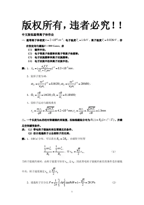
版权所有,违者必究!!中文版低温等离子体作业一. 氩等离子体密度103210n cm -=⨯, 电子温度 1.0e T eV =, 离子温度0.026i T eV =, 存在恒定均匀磁场B = 800 Gauss, 求 (1) 德拜半径;(2) 电子等离子体频率和离子等离子体频率; (3) 电子回旋频率和离子回旋频率; (4) 电子回旋半径和离子回旋半径。
解:1、1/2302()8.310()e iD e i T T mm T T neελ-==⨯+, 2、氩原子量为40,221/21/200()8.0,()29pe pi e ine ne GHz MHz m m ωωεε====,3、14,0.19e i e ieB eB GHz MHz m m Ω==Ω== 4、设粒子运动与磁场垂直24.210, 1.3e e i i ce ci m v m v r mm r mm qB qB -===⨯===二、一个长度为2L 的柱对称磁镜约束装置,沿轴线磁场分布为220()(1/)B z B z L =+,并满足空间缓变条件。
求:(1)带电粒子能被约束住需满足的条件。
(2)估计逃逸粒子占全部粒子的比例。
解:1、由B(z)分布,可以求出02m B B =,由磁矩守恒得22001122m mmv mv B B ⊥⊥=,即0m v ⊥⊥= (1) 当粒子能被约束时,由粒子能量守恒有0m v v ⊥≥,因此带电粒子能被约束住的条件是在磁镜中央,粒子速度满足002v v ⊥≥2、逃逸粒子百分比201sin 129.3%2P d d πθϕθθπ===⎰⎰ (2)三、 在高频电场0cos E E t ω=中,仅考虑电子与中性粒子的弹性碰撞,并且碰撞频率/t t ea ea v νλ=正比于速度。
求电子的速度分布函数,电子平均动能,并说明当t ea ων>>时,电子遵守麦克斯韦尔分布。
解:课件6.6节。

Gateway to control countless popular productsDesigned from the ground up to be a seamless part of URC’s Total Control® system, the TRF-ZW1 provides a gate-way to allow control of Z-Wave®-enabled products. Enjoy control of Z-Wave door locks, lighting and more from any Total Control interface including remotes, keypads and smart phones or tablets. This piece opens up Total Controlto the broadly appeal-ing world of Z-Wave integration providing yet another avenue to take total control of more components in and around your workplace with URC.TRF-ZW1TOTAL CONTROL Z-WAVE® EXTENDERCOMMERCIALTRF-ZW1TOTAL CONTROL Z-WAVE EXTENDERKeep your eye on things at workUsing URC’s handheld remotes or brilliant in-wall touch-screens, you can securely lock and unlock the doors or adjust lighting while at work. Or, using your iPad® or iPhone®, you can check on things and adjust them from afar. It’s the ideal solution for true access control. Just imagine the luxury of a completely wired o ce where all electronics talk to each other, and to you, via URC Total Control interfaces for the workplace of the future.© 2014 Universal Remote Control, Inc.WE GIVE YOU TOTAL CONTROL.Universal Remote Control, Inc. 500 Mamaroneck Ave. Harrison, NY 10528Phone (914) 835-4484 Fax (914) 835-4532 TRF-ZW1 COMMERCIAL JUNE 2014TRF-ZW1 operates on the Z-Wave frequency that’s used in the USA, Canada and Mexico (908.4 MHz). TRF-ZW is sold separately from Total Control system and interface products. Speci cations and screen designs are subject to change without notice. Universal Remote Control and Total Control are trademarks of Universal Remote Control, Inc. All other trademarks are the property of their respective owners.Two-way control of Z-Wave locks and lighting and one-way control for all Z-Wave-enabled products.Compatible with URC’s Total Control product lineSystem Integration with URC ProductsPlease note: URC two-way communication modules with speci c Z-Wave-enabled products are added in an ongoing way. To nd out if a speci c model or category of products is compatible using two-way control, please check with your URC Product Specialist, Salesperson or Tech Support. Not compatible with URC’s Complete Control™ product line.。

Spin-orbital interaction尤其是,我们讨论了在偏振螺旋光束中的纵向和轨道角动量(和平均角动量方向平行)。
然后,我们集中讨论横向(和平均角动量方向正交)自旋轨道角动量(原理和实验上都得到了讨论和观察到)。
横向自旋轨道角动量在:1、倏逝波(evanescent waves),2、交界面场(interference fields),3、聚焦光束中(focused beams)尤其是,倏逝波可以在交界面产生robust自旋轨道耦合效应(称为光的量子自旋霍尔效应)横向轨道角动量:分为extrinsic 和intrinsic.这两种轨道角动量分别由光束的空间(偏移)相移和洛伦茨根(Lotrentz boosts)产生。
The former (extrinsic) case is related to transverse shifts of paraxial beams, and it plays an important role in the spin Hall effect of light. The latter (intrinsic) case is realized in polychromatic spatio-temporal beams, which can be obtained, e.g., via a transverse Lorentz boost to a moving reference frame.目录1、简介。
22、自旋轨道角动量的基本性质。
33、横向自旋角动量。
114、横向轨道角动量。
265、结论。
33自旋角动量由圆偏振光束产生左旋右旋圆偏振光分别对应:光子的正的和负的螺旋系数(圆偏振度):σ=±1。
光的自旋角动量和光的传播方向是一致的。
Spin AM<S>=σ<k>/k(k为平均波矢)沿着光束轴的轨道角动量:<L>=l<k>/k, l光涡流的量子数(拓扑电流)。

光学专业英语50句翻译1.The group's activities in this area have concentrated on the mechanicaleffects of angular momentum on a dielectric and on the quantum properties of orbital angular momentum.在这个研究领域,这个研究组主要集中在电介质中的角动量的机械效应和轨道角动量的量子属性。
2. Experimental realization of entanglement have been restricted totwo-state quantum systems. In this experiment entanglement exploiting the orbital angular momentum of photons, which are states of the electromagnetic field with phase singularities (doughnut modes).纠缠的实验认识还只停留在二维量子系统。
在这实验中,利用了光子的轨道角动量的纠缠是具有相位奇点(暗中空模式)的电磁场的状态。
3. Laguerre Gaussian modes with an index l carry an orbital angular momentum of per photon for linearly polarized light that is distinct from the angular momentum of the photons associated with their polarization对线偏振光来说,具有因子l的LG模式的每个光子能携带的轨道角动量,这是与偏振态相关的光子的角动量是截然不同的。
十字交叉梁模型的塑性动力响应计算方法杨棣;姚熊亮;王军;李卓【摘要】The hull grillage beam’s plastic dynamic response in underwater explosion is one of the most important work in the study of anti-explosion performance. The precision of the finite element method used to solve the problem cannot be guaranteed, and the analytic method has technical difficulties. In view of that, a kind of deflection deformation calculation method that hull grillage beam was simplified into a rigid-plastic cross beam, and there is force acted on the correlation place of in the transverse and longitudinal member is put forward, through the theorem of momentum and the moment of momentum constant motion e-quation. Finally, by using this method to calculate the data, the results agree well with the test ’s and this proves that the selection of the mechanical model is rational, and illustrates that the calculation method, used for the hull grillage beam’s deflection of non-contact underwater explosion, which guarantees the cal-culation efficiency and precision, has engineering practicability.%船体板架在水下爆炸载荷作用下的塑性动力响应计算是舰船抗爆性能研究中的一项重要工作,鉴于有限元法对其求解的计算效率无法保证,同时解析法对其求解有技术上的困难等研究现状,提出了一种将船体板架结构简化成刚塑性十字交叉梁,并通过动量定理和动量矩定理由运动方程推导出十字交叉梁结构中横向和纵向构件二者在关联处有力的相互作用时的变形挠度的计算方法。
光学专业英语50句翻译1.The group's activities in this area have concentrated on the mechanicaleffects of angular momentum on a dielectric and on the quantum properties of orbital angular momentum.在这个研究领域,这个研究组主要集中在电介质中的角动量的机械效应和轨道角动量的量子属性。
2. Experimental realization of entanglement have been restricted totwo-state quantum systems. In this experiment entanglement exploiting the orbital angular momentum of photons, which are states of the electromagnetic field with phase singularities (doughnut modes).纠缠的实验认识还只停留在二维量子系统。
在这实验中,利用了光子的轨道角动量的纠缠是具有相位奇点(暗中空模式)的电磁场的状态。
3. Laguerre Gaussian modes with an index l carry an orbital angular momentum of per photon for linearly polarized light that is distinct from the angular momentum of the photons associated with their polarization对线偏振光来说,具有因子l的LG模式的每个光子能携带的轨道角动量,这是与偏振态相关的光子的角动量是截然不同的。
a rXiv:h ep-th/04121v12O ct24SLAC–PUB–10739,IPPP/04/59,DCPT/04/118,UCLA/04/TEP/40Saclay/SPhT–T04/116,hep-th/0410021October,2004N =4Super-Yang-Mills Theory,QCD and Collider Physics Z.Bern a L.J.Dixon b 1 D.A.Kosower c a Department of Physics &Astronomy,UCLA,Los Angeles,CA 90095-1547,USA b SLAC,Stanford University,Stanford,CA 94309,USA,and IPPP,University of Durham,Durham DH13LE,England c Service de Physique Th´e orique,CEA–Saclay,F-91191Gif-sur-Yvette cedex,France1Introduction and Collider Physics MotivationMaximally supersymmetric (N =4)Yang-Mills theory (MSYM)is unique in many ways.Its properties are uniquely specified by the gauge group,say SU(N c ),and the value of the gauge coupling g .It is conformally invariant for any value of g .Although gravity is not present in its usual formulation,MSYMis connected to gravity and string theory through the AdS/CFT correspon-dence[1].Because this correspondence is a weak-strong coupling duality,it is difficult to verify quantitatively for general observables.On the other hand, such checks are possible and have been remarkably successful for quantities protected by supersymmetry such as BPS operators[2],or when an additional expansion parameter is available,such as the number offields in sequences of composite,large R-charge operators[3,4,5,6,7,8].It is interesting to study even more observables in perturbative MSYM,in order to see how the simplicity of the strong coupling limit is reflected in the structure of the weak coupling expansion.The strong coupling limit should be even simpler when the large-N c limit is taken simultaneously,as it corresponds to a weakly-coupled supergravity theory in a background with a large radius of curvature.There are different ways to study perturbative MSYM.One approach is via computation of the anomalous dimensions of composite,gauge invariant operators[1,3,4,5,6,7,8].Another possibility[9],discussed here,is to study the scattering amplitudes for(regulated)plane-wave elementaryfield excitations such as gluons and gluinos.One of the virtues of the latter approach is that perturbative MSYM scat-tering amplitudes share many qualitative properties with QCD amplitudes in the regime probed at high-energy colliders.Yet the results and the computa-tions(when organized in the right way)are typically significantly simpler.In this way,MSYM serves as a testing ground for many aspects of perturbative QCD.MSYM loop amplitudes can be considered as components of QCD loop amplitudes.Depending on one’s point of view,they can be considered either “the simplest pieces”(in terms of the rank of the loop momentum tensors in the numerator of the amplitude)[10,11],or“the most complicated pieces”in terms of the degree of transcendentality(see section6)of the special functions entering thefinal results[12].As discussed in section6,the latter interpreta-tion links recent three-loop anomalous dimension results in QCD[13]to those in the spin-chain approach to MSYM[5].The most direct experimental probes of short-distance physics are collider experiments at the energy frontier.For the next decade,that frontier is at hadron colliders—Run II of the Fermilab Tevatron now,followed by startup of the CERN Large Hadron Collider in2007.New physics at colliders always contends with Standard Model backgrounds.At hadron colliders,all physics processes—signals and backgrounds—are inherently QCD processes.Hence it is important to be able to predict them theoretically as precisely as possi-ble.The cross section for a“hard,”or short-distance-dominated processes,can be factorized[14]into a partonic cross section,which can be computed order by order in perturbative QCD,convoluted with nonperturbative but measur-able parton distribution functions(pdfs).For example,the cross section for producing a pair of jets(plus anything else)in a p¯p collision is given byσp¯p→jjX(s)= a,b1 0dx1dx2f a(x1;µF)¯f b(x2;µF)׈σab→jjX(sx1x2;µF,µR;αs(µR)),(1)where s is the squared center-of-mass energy,x1,2are the longitudinal(light-cone)fractions of the p,¯p momentum carried by partons a,b,which may be quarks,anti-quarks or gluons.The experimental definition of a jet is an in-volved one which need not concern us here.The pdf f a(x,µF)gives the prob-ability forfinding parton a with momentum fraction x inside the proton; similarly¯f b is the probability forfinding parton b in the antiproton.The pdfs depend logarithmically on the factorization scaleµF,or transverse resolution with which the proton is examined.The Mellin moments of f a(x,µF)are for-ward matrix elements of leading-twist operators in the proton,renormalized at the scaleµF.The quark distribution function q(x,µ),for example,obeys 10dx x j q(x,µ)= p|[¯qγ+∂j+q](µ)|p .2Ingredients for a NNLO CalculationMany hadron collider measurements can benefit from predictions that are accurate to next-to-next-to-leading order(NNLO)in QCD.Three separate ingredients enter such an NNLO computation;only the third depends on the process:(1)The experimental value of the QCD couplingαs(µR)must be determinedat one value of the renormalization scaleµR(for example m Z),and its evolution inµR computed using the3-loopβ-function,which has been known since1980[15].(2)The experimental values for the pdfs f a(x,µF)must be determined,ide-ally using predictions at the NNLO level,as are available for deep-inelastic scattering[16]and more recently Drell-Yan production[17].The evolu-tion of pdfs inµF to NNLO accuracy has very recently been completed, after a multi-year effort by Moch,Vermaseren and Vogt[13](previously, approximations to the NNLO kernel were available[18]).(3)The NNLO terms in the expansion of the partonic cross sections must becomputed for the hadronic process in question.For example,the parton cross sections for jet production has the expansion,ˆσab→jjX=α2s(A+αs B+α2s C+...).(2)The quantities A and B have been known for over a decade[19],but C has not yet been computed.Figure 1.LHC Z production [22].•real ×real:וvirtual ×real:וvirtual ×virtual:וdoubly-virtual ×real:×Figure 2.Purely gluonic contributionsto ˆσgg →jjX at NNLO.Indeed,the NNLO terms are unknown for all but a handful of collider puting a wide range of processes at NNLO is the goal of a large amount of recent effort in perturbative QCD [20].As an example of the im-proved precision that could result from this program,consider the production of a virtual photon,W or Z boson via the Drell-Yan process at the Tevatron or LHC.The total cross section for this process was first computed at NNLO in 1991[21].Last year,the rapidity distribution of the vector boson also be-came available at this order [17,22],as shown in fig.1.The rapidity is defined in terms of the energy E and longitudinal momentum p z of the vector boson in the center-of-mass frame,Y ≡1E −p z .It determines where the vector boson decays within the detector,or outside its acceptance.The rapidity is sensitive to the x values of the incoming partons.At leading order in QCD,x 1=e Y m V /√s ,where m V is the vector boson mass.The LHC will produce roughly 100million W s and 10million Z s per year in detectable (leptonic)decay modes.LHC experiments will be able to map out the curve in fig.1with exquisite precision,and use it to constrain the parton distributions —in the same detectors that are being used to search for new physics in other channels,often with similar q ¯q initial states.By taking ratios of the other processes to the “calibration”processes of single W and Z production,many experimental uncertainties,including those associated with the initial state parton distributions,drop out.Thus fig.1plays a role as a “partonic luminosity monitor”[23].To get the full benefit of the remarkable experimental precision,though,the theory uncertainty must approach the 1%level.As seen from the uncertainty bands in the figure,this precision is only achievable at NNLO.The bands are estimated by varying the arbitrary renormalization and factorization scales µR and µF (set to a common value µ)from m V /2to 2m V .A computation to all orders in αs would have no dependence on µ.Hence the µ-dependence of a fixed order computation is related to the size of the missing higher-order terms in the series.Althoughsub-1%uncertainties may be special to W and Z production at the LHC, similar qualitative improvements in precision will be achieved for many other processes,such as di-jet production,as the NNLO terms are completed.Even within the NNLO terms in the partonic cross section,there are several types of ingredients.This feature is illustrated infig.2for the purely gluonic contributions to di-jet production,ˆσgg→jjX.In thefigure,individual Feynman graphs stand for full amplitudes interfered(×)with other amplitudes,in order to produce contributions to a cross section.There may be2,3,or4partons in thefinal state.Just as in QED it is impossible to define an outgoing electron with no accompanying cloud of soft photons,also in QCD sensible observables require sums overfinal states with different numbers of partons.Jets,for example,are defined by a certain amount of energy into a certain conical region.At leading order,that energy typically comes from a single parton, but at NLO there may be two partons,and at NNLO three partons,within the jet cone.Each line infig.2results in a cross-section contribution containing severe infrared divergences,which are traditionally regulated by dimensional regula-tion with D=4−2ǫ.Note that this regulation breaks the classical conformal invariance of QCD,and the classical and quantum conformal invariance of N=4super-Yang-Mills theory.Each contribution contains poles inǫranging from1/ǫ4to1/ǫ.The poles in the real contributions come from regions ofphase-space where the emitted gluons are soft and/or collinear.The poles in the virtual contributions come from similar regions of virtual loop integra-tion.The virtual×real contribution obviously has a mixture of the two.The Kinoshita-Lee-Nauenberg theorem[24]guarantees that the poles all cancel in the sum,for properly-defined,short-distance observables,after renormal-izing the coupling constant and removing initial-state collinear singularities associated with renormalization of the pdfs.A critical ingredient in any NNLO prediction is the set of two-loop ampli-tudes,which enter the doubly-virtual×real interference infig.2.Such ampli-tudes require dimensionally-regulated all-massless two-loop integrals depend-ing on at least one dimensionless ratio,which were only computed beginning in 1999[25,26,27].They also receive contributions from many Feynman diagrams, with lots of gauge-dependent cancellations between them.It is of interest to develop more efficient,manifestly gauge-invariant methods for combining di-agrams,such as the unitarity or cut-based method successfully applied at one loop[10]and in the initial two-loop computations[28].i,ij+ i iFigure3.Illustration of soft-collinear(left)and pure-collinear(right)one-loop di-vergences.3N=4Super-Yang-Mills Theory as a Testing Ground for QCDN=4super-Yang-Mills theory serves an excellent testing ground for pertur-bative QCD methods.For n-gluon scattering at tree level,the two theories in fact give identical predictions.(The extra fermions and scalars of MSYM can only be produced in pairs;hence they only appear in an n-gluon ampli-tude at loop level.)Therefore any consequence of N=4supersymmetry,such as Ward identities among scattering amplitudes[29],automatically applies to tree-level gluonic scattering in QCD[30].Similarly,at tree level Witten’s topological string[31]produces MSYM,but implies twistor-space localization properties for QCD tree amplitudes.(Amplitudes with quarks can be related to supersymmetric amplitudes with gluinos using simple color manipulations.)3.1Pole Structure at One and Two LoopsAt the loop-level,MSYM becomes progressively more removed from QCD. However,it can still illuminate general properties of scattering amplitudes,in a calculationally simpler arena.Consider the infrared singularities of one-loop massless gauge theory amplitudes.In dimensional regularization,the leading singularity is1/ǫ2,arising from virtual gluons which are both soft and collinear with respect to a second gluon or another massless particle.It can be char-acterized by attaching a gluon to any pair of external legs of the tree-level amplitude,as in the left graph infig.3.Up to color factors,this leading diver-gence is the same for MSYM and QCD.There are also purely collinear terms associated with individual external lines,as shown in the right graph infig.3. The pure-collinear terms have a simpler form than the soft terms,because there is less tangling of color indices,but they do differ from theory to theory.The full result for one-loop divergences can be expressed as an operator I(1)(ǫ) which acts on the color indices of the tree amplitude[32].Treating the L-loop amplitude as a vector in color space,|A(L)n ,the one-loop result is|A(1)n =I(1)(ǫ)|A(0)n +|A(1),finn ,(3)where |A (1),fin nis finite as ǫ→0,and I (1)(ǫ)=1Γ(1−ǫ)n i =1n j =i T i ·T j 1T 2i 1−s ij ǫ,(4)where γis Euler’s constant and s ij =(k i +k j )2is a Mandelstam invariant.The color operator T i ·T j =T a i T a j and factor of (µ2R /(−s ij ))ǫarise from softgluons exchanged between legs i and j ,as in the left graph in fig.3.The pure 1/ǫpoles terms proportional to γi have been written in a symmetric fashion,which slightly obscures the fact that the color structure is actually simpler.We can use the equation which represents color conservation in the color-space notation, n j =1T j =0,to simplify the result.At order 1/ǫwe may neglect the (µ2R /(−s ij ))ǫfactor in the γi terms,and we have n j =i T i ·T j γi /T 2i =−γi .So the color structure of the pure 1/ǫterm is actually trivial.For an n -gluon amplitude,the factor γi is set equal to its value for gluons,which turns out to be γg =b 0,the one-loop coefficient in the β-function.Hence the pure-collinear contribution vanishes for MSYM,but not for QCD.The divergences of two-loop amplitudes can be described in the same for-malism [32].The relation to soft-collinear factorization has been made more transparent by Sterman and Tejeda-Yeomans,who also predicted the three-loop behavior [33].Decompose the two-loop amplitude |A (2)n as|A (2)n =I (2)(ǫ)|A (0)n +I (1)(ǫ)|A (1)n +|A (2),fin n,(5)where |A (2),fin n is finite as ǫ→0and I (2)(ǫ)=−1ǫ+e −ǫγΓ(1−2ǫ)ǫ+K I (1)(2ǫ)+e ǫγT 2i µ22C 2A ,(8)where C A =N c is the adjoint Casimir value.The quantity ˆH(2)has non-trivial,but purely subleading-in-N c ,color structure.It is associated with soft,rather than collinear,momenta [37,33],so it is theory-independent,up to color factors.An ansatz for it for general n has been presented recently [38].3.2Recycling Cuts in MSYMAn efficient way to compute loop amplitudes,particularly in theories with a great deal of supersymmetry,is to use unitarity and reconstruct the am-plitude from its cuts [10,38].For the four-gluon amplitude in MSYM,the two-loop structure,and much of the higher-loop structure,follows from a sim-ple property of the one-loop two-particle cut in this theory.For simplicity,we strip the color indices offof the four-point amplitude A (0)4,by decomposing it into color-ordered amplitudes A (0)4,whose coefficients are traces of SU(N c )generator matrices (Chan-Paton factors),A (0)4(k 1,a 1;k 2,a 2;k 3,a 3;k 4,a 4)=g 2 ρ∈S 4/Z 4Tr(T a ρ(1)T a ρ(2)T a ρ(3)T a ρ(4))×A (0)4(k ρ(1),k ρ(2),k ρ(3),k ρ(4)).(9)The two-particle cut can be written as a product of two four-point color-ordered amplitudes,summed over the pair of intermediate N =4states S,S ′crossing the cut,which evaluates toS,S ′∈N =4A (0)4(k 1,k 2,ℓS ,−ℓ′S ′)×A (0)4(ℓ′S ′,−ℓS ,k 3,k 4)=is 12s 23A (0)4(k 1,k 2,k 3,k 4)×1(ℓ−k 3)2,(10)where ℓ′=ℓ−k 1−k 2.This equation is also shown in fig.4.The scalar propagator factors in eq.(10)are depicted as solid vertical lines in the figure.The dashed line indicates the cut.Thus the cut reduces to the cut of a scalar box integral,defined byI D =4−2ǫ4≡ d 4−2ǫℓℓ2(ℓ−k 1)2(ℓ−k 1−k 2)2(ℓ+k 4)2.(11)One of the virtues of eq.(10)is that it is valid for arbitrary external states in the N =4multiplet,although only external gluons are shown in fig.4.Therefore it can be re-used at higher loop order,for example by attaching yet another tree to the left.N =41234=i s 12s 231234Figure 4.The one-loop two-particle cuts for the four-point amplitude in MSYM reduce to the tree amplitude multiplied by a cut scalar box integral (for any set of four external states).i 2s 12s121234+s 121234+perms Figure 5.The two-loop gg →gg amplitude in MSYM [11,39].The blob on theright represents the color-ordered tree amplitude A (0)4.(The quantity s 12s 23A (0)4transforms symmetrically under gluon interchange.)In the the brackets,black linesare kinematic 1/p 2propagators,with scalar (φ3)vertices.Green lines are color δab propagators,with structure constant (f abc )vertices.The permutation sum is over the three cyclic permutations of legs 2,3,4,and makes the amplitude Bose symmetric.At two loops,the simplicity of eq.(10)made it possible to compute the two-loop gg →gg scattering amplitude in that theory (in terms of specific loop integrals)in 1997[11],four years before the analogous computations in QCD [36,37].All of the loop momenta in the numerators of the Feynman di-agrams can be factored out,and only two independent loop integrals appear,the planar and nonplanar scalar double box integrals.The result can be writ-ten in an appealing diagrammatic form,fig.5,where the color algebra has the same form as the kinematics of the loop integrals [39].At higher loops,eq.(10)leads to a “rung rule”[11]for generating a class of (L +1)-loop contributions from L -loop contributions.The rule states that one can insert into a L -loop contribution a rung,i.e.a scalar propagator,transverse to two parallel lines carrying momentum ℓ1+ℓ2,along with a factor of i (ℓ1+ℓ2)2in the numerator,as shown in fiing this rule,one can construct recursively the external and loop-momentum-containing numerators factors associated with every φ3-type diagram that can be reduced to trees by a sequence of two-particle cuts,such as the diagram in fig.7a .Such diagrams can be termed “iterated 2-particle cut-constructible,”although a more compact notation might be ‘Mondrian’diagrams,given their resemblance to Mondrian’s paintings.Not all diagrams can be computed in this way.The diagram in fig.7b is not in the ‘Mondrian’class,so it cannot be determined from two-particle cuts.Instead,evaluation of the three-particle cuts shows that it appears with a non-vanishing coefficient in the subleading-color contributions to the three-loop MSYM amplitude.ℓ1ℓ2−→i (ℓ1+ℓ2)2ℓ1ℓ2Figure 6.The rung rule for MSYM.(a)(b)Figure 7.(a)Example of a ‘Mondrian’diagram which can be determined re-cursively from the rung rule.(b)Thefirst non-vanishing,non-Mondrian dia-grams appear at three loops in nonplanar,subleading-color contributions.4Iterative Relation in N =4Super-Yang-Mills TheoryAlthough the two-loop gg →gg amplitude in MSYM was expressed in terms of scalar integrals in 1997[11],and the integrals themselves were computed as a Laurent expansion about D =4in 1999[25,26],the expansion of the N =4amplitude was not inspected until last fall [9],considerably after similar investigations for QCD and N =1super-Yang-Mills theory [36,37].It was found to have a quite interesting “iterative”relation,when expressed in terms of the one-loop amplitude and its square.At leading color,the L -loop gg →gg amplitude has the same single-trace color decomposition as the tree amplitude,eq.(9).Let M (L )4be the ratio of this leading-color,color-ordered amplitude to the corresponding tree amplitude,omitting also several conventional factors,A (L ),N =4planar 4= 2e −ǫγg 2N c2 M (1)4(ǫ) 2+f (ǫ)M (1)4(2ǫ)−12(ζ2)2is replaced by approximately sixpages of formulas (!),including a plethora of polylogarithms,logarithms and=+f(ǫ)−12(ζ2)2+O(ǫ)f(ǫ)=−(ζ2+ǫζ3+ǫ2ζ4+...)Figure8.Schematic depiction of the iterative relation(13)between two-loop and one-loop MSYM amplitudes.polynomials in ratios of invariants s/t,s/u and t/u[37].The polylogarithm is defined byLi m(x)=∞i=1x i t Li m−1(t),Li1(x)=−ln(1−x).(14)It appears with degree m up to4at thefinite,orderǫ0,level;and up to degree4−i in the O(ǫ−i)terms.In the case of MSYM,identities relating these polylogarithms are needed to establish eq.(13).Although the O(ǫ0)term in eq.(13)is miraculously simple,as noted above the behavior of the pole terms is not a miracle.It is dictated in general terms by the cancellation of infrared divergences between virtual corrections and real emission[24].Roughly speaking,for this cancellation to take place,the virtual terms must resemble lower-loop amplitudes,and the real terms must resemble lower-point amplitudes,in the soft and collinear regions of loop or phase-space integration.At the level of thefinite terms,the iterative relation(13)can be understood in the Regge/BFKL limit where s≫t,because it then corresponds to expo-nentiation of large logarithms of s/t[40].For general values of s/t,however, there is no such argument.The relation is special to D=4,where the theory is conformally invariant. That is,the O(ǫ1)remainder terms cannot be simplified significantly.For ex-ample,the two-loop amplitude M(2)4(ǫ)contains at O(ǫ1)all three independent Li5functions,Li5(−s/u),Li5(−t/u)and Li5(−s/t),yet[M(1)4(ǫ)]2has only the first two of these[9].The relation is also special to the planar,leading-color limit.The subleading color-components of thefinite remainder|A(2),finn defined by eq.(5)show no significant simplification at all.For planar amplitudes in the D→4limit,however,there is evidence that an identical relation also holds for an arbitrary number n of external legs, at least for certain“maximally helicity-violating”(MHV)helicity amplitudes. This evidence comes from studying the limits of two-loop amplitudes as two of the n gluon momenta become collinear[9,38,41].(Indeed,it was by analyzing these limits that the relation for n=4wasfirst uncovered.)The collinear limits turn out to be consistent with the same eq.(13)with M4replaced by M n everywhere[9],i.e.M(2)n(ǫ)=12(ζ2)2+O(ǫ).(15)The collinear consistency does not constitute a proof of eq.(15),but in light of the remarkable properties of MSYM,it would be surprising if it were not true in the MHV case.Because the direct computation of two-loop amplitudes for n>4seems rather difficult,it would be quite interesting to try to examine the twistor-space properties of eq.(15),along the lines of refs.[31,42].(The right-hand-side of eq.(15)is not completely specified at order1/ǫandǫ0for n>4.The reason is that the orderǫandǫ2terms in M(1)n(ǫ),which contribute to thefirst term in eq.(15)at order1/ǫandǫ0,contain the D=6−2ǫpentagon integral[43],which is not known in closed form.On the other hand, the differential equations this integral satisfies may suffice to test the twistor-space behavior.Or one may examine just thefinite remainder M(L),finn definedvia eq.(5).)It may soon be possible to test whether an iterative relation for planar MSYM amplitudes extends to three loops.An ansatz for the three-loop planar gg→gg amplitude,shown infig.9,was provided at the same time as the two-loop re-sult,in1997[11].The ansatz is based on the“rung-rule”evaluation of the iterated2-particle cuts,plus the3-particle cuts with intermediate states in D=4;the4-particle cuts have not yet been verified.Two integrals,each be-ginning at O(ǫ−6),are required to evaluate the ansatz in a Laurent expansion about D=4.(The other two integrals are related by s↔t.)The triple ladder integral on the top line offig.9was evaluated last year by Smirnov,all the way through O(ǫ0)[44].Evaluation of the remaining integral,which contains a factor of(ℓ+k4)2in the numerator,is in progress[45];all the terms through O(ǫ−2)agree with predictions[33],up to a couple of minor corrections.5Significance of Iterative Behavior?It is not yet entirely clear why the two-loop four-point amplitude,and prob-ably also the n-point amplitudes,have the iterative structure(15).However, one can speculate that it is from the need for the perturbative series to=i3s12s212+s223+2s12(ℓ+k4)+2s23(ℓ+k1)21Figure9.Graphical representation of the three-loop amplitude for MSYM in the planar limit.be summable into something which becomes“simple”in the planar strong-coupling limit,since that corresponds,via AdS/CFT,to a weakly-coupled supergravity theory.The fact that the relation is special to the conformal limit D→4,and to the planar limit,backs up this speculation.Obviously it would be nice to have some more information at three loops.There have been other hints of an iterative structure in the four-point correlation func-tions of chiral primary(BPS)composite operators[46],but here also the exact structure is not yet clear.Integrability has played a key role in recent higher-loop computations of non-BPS spin-chain anomalous dimensions[4,5,6,8].By imposing regularity of the BMN‘continuum’limit[3],a piece of the anoma-lous dimension matrix has even been summed to all orders in g2N c in terms of hypergeometric functions[7].The quantities we considered here—gauge-invariant,but dimensionally regularized,scattering amplitudes of color non-singlet states—are quite different from the composite color-singlet operators usually treated.Yet there should be some underlying connection between the different perturbative series.6Aside:Anomalous Dimensions in QCD and MSYMAs mentioned previously,the set of anomalous dimensions for leading-twist operators was recently computed at NNLO in QCD,as the culmination of a multi-year effort[13]which is central to performing precise computations of hadron collider cross sections.Shortly after the Moch,Vermaseren and Vogt computation,the anomalous dimensions in MSYM were extracted from this result by Kotikov,Lipatov,Onishchenko and Velizhanin[12].(The MSYM anomalous dimensions are universal;supersymmetry implies that there is only one independent one for each Mellin moment j.)This extraction was non-trivial,because MSYM contains scalars,interacting through both gauge and Yukawa interactions,whereas QCD does not.However,Kotikov et al.noticed, from comparing NLO computations in both leading-twist anomalous dimen-sions and BFKL evolution,that the“most complicated terms”in the QCDcomputation always coincide with the MSYM result,once the gauge group representation of the fermions is shifted from the fundamental to the adjoint representation.One can define the“most complicated terms”in the x-space representation of the anomalous dimensions—i.e.the splitting kernels—as follows:Assign a logarithm or factor ofπa transcendentality of1,and a polylogarithm Li m or factor ofζm=Li m(1)a transcendentality of m.Then the most complicated terms are those with leading transcendentality.For the NNLO anomalous dimensions,this turns out to be transcendentality4.(This rule for extracting the MSYM terms from QCD has also been found to hold directly at NNLO,for the doubly-virtual contributions[38].)Strikingly,the NNLO MSYM anomalous dimension obtained for j=4by this procedure agrees with a previous result derived by assuming an integrable structure for the planar three-loop contribution to the dilatation operator[5].7Conclusions and OutlookN=4super-Yang-Mills theory is an excellent testing ground for techniques for computing,and understanding the structure of,QCD scattering amplitudes which are needed for precise theoretical predictions at high-energy colliders. One can even learn something about the structure of N=4super-Yang-Mills theory in the process,although clearly there is much more to be understood. Some open questions include:Is there any AdS/CFT“dictionary”for color non-singlet states,like plane-wave gluons?Can one recover composite operator correlation functions from any limits of multi-point scattering amplitudes?Is there a better way to infrared regulate N=4supersymmetric scattering amplitudes,that might be more convenient for approaching the AdS/CFT correspondence,such as compactification on a three-sphere,use of twistor-space,or use of coherent external states?Further investigations of this arena will surely be fruitful.AcknowledgementsWe are grateful to the organizers of Strings04for putting together such a stim-ulating meeting.This research was supported by the US Department of En-ergy under contracts DE-FG03-91ER40662(Z.B.)and DE-AC02-76SF00515 (L.J.D.),and by the Direction des Sciences de la Mati`e re of the Commissariat `a l’Energie Atomique of France(D.A.K.).。
abort异常中断,中途失败,夭折,流产,发育不全,中止计划[任务]accidentally偶然地,意外地accretion 增长activation energy 活化能active center活性中心addition 增加adjacent相邻的aerosol浮质(气体中的悬浮微粒,如烟,雾等),[化]气溶胶,气雾剂,烟雾剂Air flow circuits 气流循环ambient周国的,周用环境amines 胺amplitude广阔,丰富,振幅,物理学名词annular环流的algebraic stress model(ASM)代数应力模型algorithm 算法align排列,使结盟,使成一行alternately 轮流地analogy模拟,效仿analytical solution 解析解anisotropic各向异性的anthracite 无烟煤apparent显然的,外观上的,近似的approximation 近似arsenic神酸盐assembly 装配associate 联合,联系assume假设assumption 假设atomization 雾化axial轴向的Axisymmetry轴对称的BBaffle挡流板battlement 城垛式biography 经历bituminous coal 烟煤blow-off water 排污水blowing devices鼓风(吹风)装置body force体积力boiler plant锅炉装置(车间)Boiling 沸腾Boltzmann玻耳兹曼Bounded central differencing:有界中心差分格式Brownian rotation 布朗转动bulk庞大的bulk density堆积密度burner assembly燃烧器组件burnout 燃尽Ccapability性能,(实际)能力,容量,接受力carbon monoxide COcarbonate碳酸盐carry-over loss 飞灰损失Cartesian迪卡尔坐标的casing箱,壳,套catalisis 催化channeled有沟的,有缝的char焦炭、炭circulation circuit 循环回路circumferential velocity 圆周速度clinkering 熔渣clipped截尾的clipped Gaussian distribution 截尾髙斯分布closure (模型的)封闭cloud of particles 颗粒云close proximity 距离很近cluster颗粒团coal off-gas煤的挥发气体coarse粗糙的coarse grid疏网格,粗网格Coatingcoaxial R 轴的coefficient of restitution 回弹系数;恢复系数coke 碳collision 碰撞competence 能力competing process同时发生影响的competing-reactions submodel 平行反应子模型component部分分量composition 成分computational expense 计算成本cone shape圆锥体形状configuration 布置,构造confined flames 有界燃烧confirmation证实,确认,批准Configuration 构造,外形conservation守恒不火conservation equation 守恒方程conserved scalars 守恒标量considerably 相当地consume 消耗contact angle 接触角contamination 污染contingency偶然,可能性,意外事故,可能发生的附带事件continuum连续体Convection 对流converged收敛的conveyer输运机convolve 卷cooling wall 水冷壁correlation 关联(式)correlation function 相关函数corrosion 腐蚀,锈coupling联结,接合,耦合crack裂缝,裂纹creep up (水)渗上来,蠕升critical 临界critically 精密地cross-correlation 互关联cumulative 累积的curtain wall护墙,幕墙curve曲线custom习惯,风俗,<动词单用〉海关,(封建制度下)左期服劳役,缴纳租税,自定义,v偶用作〉关税V.定制,承接左做活的Cyan青色cyano叙(基),深蓝,青色cyclone旋风子,旋风,旋风筒cyclone separator旋风分离器[除尘器]cylindrical柱坐标的cylindrical coordinate 柱坐标Ddead zones 死区decompose 分解decouple解藕的cooling duct 冷却管coordinate transformation 坐标转换Cp:等压比热defy 使成为不可能 demography 统计 deposition 沉枳derivative with respect to 对…的导数derivation 引出,来历,出处,(语言)语源,词源 design cycle 设计流程 desposit 积灰,结垢deterministic approach 确上轨道模型 deterministic 宿命的 deviation 偏差 devoid 缺乏devolatilization 析出挥发分,液化作用 diffusion 扩散 diffusivity 扩散系数digonal 二角(的),对角的,二维的 dilute 稀的 diminish 减少direct numerical simulation 直接数值模拟 discharge 释放 discrete 离散的discrete phase 分散相,不连续相 discretization [数]离散化 deselect 取消选泄 dispersion 弥散 dissector 扩流锥dissociate thermally 热分解 dissociation 分裂dissipation 消散,分散,挥霍,浪费,消遣,放荡,狂饮 distribution of air 布风 divide 除以 dot line 虚线drag coefficient 牵引系数,阻力系数 drag and drop 拖放 drag force 曳力 drift velocity 漂移速度 driving force 驱[传,主]动力 droplet 液滴 drum 锅筒dry-bottom-furnace 固态排渣炉 dry-bottom 冷灰斗,固态排渣 duct 管 dump 渣坑dust-air mixture 一次风 EEBU-Eddy break up 漩涡破碎模型 eddy 涡旋effluent 废气,流出物 elastic 弹性的electro-staic precipitators 静电除尘器Deforming :变形 Density :密度emanate散发,发岀,发源,[罕]发散,放射embrasure 喷口,枪眼emissivity [物]发射率empirical经验的endothermic reaction 吸热反应enhance 增,涨enlarge 扩大ensemble组,群,全体enthalpy 焰entity实体entrain携带,夹带entrained-bed 携带床Equation 方程equilibrate保持平衡equilibrium化学平衡ESCIMO——Engulfment (卷吞)Stretching (拉伸)Coherence (粘附)Interdiffusion-interaction (相互扩散和化学反应)Moving-observer (运动观察者)exhaust用尽,耗尽,抽完,使精疲力尽排气排气装巻用不完的,不会枯竭的exit出口,排气管exothermic reaction 放热反应expenditure支出,经费expertise 经验explicitly明白地,明确地extinction 熄灭的extract抽出,提取evaluation评价,估计,赋值evaporation 蒸发(作用)Eulerian approach 欧拉法Ffacilitate推动,促进factor把…分解fast chemistry快速化学反应fate天数,命运,运气,注定,送命,最终结果feasible可行的,可能的feed pump给水泵feedstock 填料Filling 倒水fine grid密网格,细网格finite difference approximation 有限差分法flamelet小火焰单元flame stability火焰稳定性flow pattern 流型fluctuating velocity 脉动速度fluctuation脉动,波动flue烟道(气)flue duck 烟道fluoride氟化物fold夹层块forced-and-induced draft fan 鼓引风机forestall 防止Formulation:公式,函数fouling 沾污fraction碎片部分,百分比fragmentation 破碎fuel-lean flamefuel-rich regions富燃料区,浓燃料区fuse熔化,熔融Ggas duct 烟道gas-tight烟气密封gasification 气化(作用)gasifier气化器Gauge厚度,直径,测量仪表,估测。
a rXiv:h ep-ph/979380v117Se p1997WW PHYSICS AT LEP2aR.MIQUEL b Dept.ECM and IFAE,Facultat de F´ısica,Univ.de Barcelona Diagonal 647,E-08028Barcelona (Spain)The analyses and results on WW physics obtained in the first year of running of LEP2are summarized.The determination of the W mass,both through the measurement of the WW production cross section at a center-of-mass energy of 161GeV and through the study of the invariant mass distribution of W decay products in the 172GeV run are described first.Preliminary results on searches for anomalous triple gauge-boson vertices are also presented.1Introduction The LEP accelerator at CERN is just in the middle of an energy upgrade that will bring its energy to about 195GeV in year 1998,with peak luminosities close to 1032cm −2s −1.The main reason to double the energy of the LEP machine is to be able to produce pairs of W’s.Their mass can be accurately measured,providing a new constraint on the Minimal Standard Model (MSM)fundamental parameters.A very precise measurement of the W mass could provide useful information on the mass of the MSM Higgs boson.The W couplings to the other vector bosons in the electroweak theory (photon and Z),which come from the non-abelian nature of the gauge group,can be studied with great detail and constraints on new physics can be derived from their determination.This article summarizes the first results on WW physics obtained with the 1996data sample and will analyse also the prospects for precise measurements of both the W mass and its couplings to Z and photon when the whole datasample will be collected around year 2000.The 1996LEP2run was splitted into two parts.The first run,between June and August 1996collected 11pb −1of data per experiment at a center-of-mass energy√s =172GeV and accumulated 10pb −1.Final results from the WW analyses for the first set are available from all four LEP experiments 1–4and will be reviewed here.At the time of writing,only preliminary results wereFigure1:Feynmann diagrams for the production and decay of a W+W−pair at LEP2. available from the172GeV run.They will also be discussed here,although with less detail,due to their volatility.The current LEP2schedule includes running in years1997–1999withcenter-of-mass enegies increasing from184GeV in1997to194GeV in1998 and1999.The expected luminosities are around100pb−1for1997and about180pb−1in each of1998and1999.Together with the21pb−1collected in1996,this would bring the total close to500pb−1,which will be taken in the following as ultimate LEP2luminosity per experiment.Section2discusses some generalities about W production and decay,selec-tion and background in e+e−collisions.The W mass determination done with 1996data taken near the WW production threshold is presented in section3.The measurement done with the1996data at higher energy(172GeV)and theprospects using all data up to1999are the subject of section4.Section5con-tains thefirst results and future capabilities of LEP2in the measurement of thetrilinear gauge-boson couplings.Finally,section6contains a brief summarywith the conclusions of the paper.2WW production and decayPairs of W+s and W−s are produced at LEP2based on the three tree-leveldiagrams depicted infig.1.The t-channel exchange diagram dominates the resulting amplitude by having a factorβ= 1−4M2W/s 1/2less.Therefore, the Ws tend to be produced in the forward direction.More so near thresh-old,whereβis indeed very small.The other two diagrams,whose existenceis needed in order to preserve unitarity,include the non-abelian couplings be-tween two Ws and either a photon or a Z.Since the t-channel diagram dom-inates near threshold,it is clear that the experimental sensitivity to trilinear2gauge-boson couplings will be higher for higher center-of-mass energies.Neglectingflavour-mixing,the W boson decays to each pair of available up-antidown fermions with the same strength.Therefore,its branching ratios are1/3to lepton and neutrino and2/3to quark-antiquark.Because of the large mass of the top quark,decays to top-bottom pair are not allowed and, therefore,neglecting bottom-strange and bottom-down mixing,no b quarks are produced in W decays.Considering now W pairs,there are three possiblefinal states:•llνν(10.5%of the total WW sample).There are at least two neutrinos (more if l=τ).The complete reconstruction of the event is possible only if the value of the W mass is assumed.These events can be used in the determination of the anomalous couplings.•lνjet jet(44%).With one neutrino(l=e,µ,30%)the complete kine-matical reconstruction is possible.These are clean events,with the two Ws clearly separated.They can be used in any study presented below.•jet jet jet jet(45.5%).Often with afifth jet due to gluon radiation.These are messy,unclear events,with important QCD backgrounds.The task of assigning particles to jets and jets to Ws is not easy.While the possibility of using the four-jet events for the determination of the W mass is by nowfirmly established,it still remains to be seen whether they can be used effectively in the anomalous couplings analysis.The two main topics of interest in W physics at LEP2are the precise de-termination of the W mass and the study of the non-abelian couplings between two Ws and Z orγ.They will be discussed in turn in the following.3W mass measurement at thresholdThe current best determination of M W comes from the CDF6,7and D08exper-iments at the Tevatron,which get the W mass through afit to the“transverse mass”distribution measured in W leptonic decays from the lepton momentum and the missing transverse momentum.Their current averaged value is7M W=80.37±0.10GeV.This number makes use of all available CDF and D0data.By the end of run II,expected to start in1999,the error could go down to30–40MeV.An indirect M W determination can be obtained from the Standard Model fits to all electroweak data,mainly LEP1results.Once the free parameters of3the minimal standard model,like m t or M H are obtained from thefit,they can be used to predict any other observable like M W.The current best value, not using the direct M W and m t information,is9M W=80.323±0.042GeV,in excellent agreement with the direct measurement.A strong consistency check of the theory can be obtained by compar-ing both numbers.The uncertainty in the indirect determination is going to decrease only slightly in the near future(thanks to the continuing sin2θW measurements at SLAC).Therefore a crucial goal for the direct M W determi-nations is to bring down the error to the30–40MeV level,comparable to the error of the indirect measurement.Two very different methods exist for the measurement of the W mass at LEP2:•Measuring the total WW production cross section near the threshold region allows the determination of the kinematical threshold and,there-fore,the W mass.The advantadges of this method is that only involves counting events,it is clean and uses all decay channels.However,it needs data very close to threshold,where the cross section is small and,thre-fore,signal to background ratios are low and the number of events(for other measurements)is minimal.•The direct reconstruction of the invariant mass of hadronic and leptonic decays uses about90%of the events(all but the ones with two lep-tonic decays)and it works equally well at any LEP2energy above about 170GeV.However,it is very involved,especially for four-jet events,and it can be sensitive to soft QCD effects,also for the four-jet channel. Both methods rely on the knowledge of the beam energy,the second because some sort of kinematicalfit assuming four-momentum conservation is needed in order to improve the invariant mass resolution.In both cases,the error on the beam energy,∆E b,translates almost directly into an error on the W mass:∆M W(beam)≃∆E b.The main problem for the measurement of the WW cross section near threshold is that the background is much larger than the signal,in particular for the fully hadronic channel.While the cross section for WW production and subsequent decay to hadrons is about1.6pb at161GeV,the cross section for hadron production through photon and/or Z reaches about150pb,or100 times more.4Studies previous to the start-up of LEP211showed that for a luminosity of100pb−1,the overall statistical error on M W could be of order134MeV. Systematic errors were thought to be considerably smaller,leading to a total uncertainty around144MeV,when considering four experiments collecting 25pb−1each.3.1The W W→lνlνchannel at161GeVThe events in which both Ws decay leptonically are very simple indeed.All experiments select these events based on their low charge and neutral mul-tiplicity,high missing transverse momentum(due to the neutrinos)and high acoplanarity(since there is more than one invisible particle).The overall ef-ficiency varies with experiment,from about40%to almost70%.Differences amongst experiments have to do with their different solid angle coverage for track measurements and their diverse capabilities in tau identification.Indeed, a big fraction of the inefficiency comes from events were at least one of the Ws decay into tau.Backgrounds are estimated to be very low,around50fb,to be compared with a signal cross section around400fb.The four experiments together have collected12events of this type.Clearly,with this level of statistics,it is not susprising that systematic errors are negligibly small,compared to the statistical error.3.2The W W→lνqq channel at161GeVThe selection of W W→lνqq when l=e,µis also very simple.All experiments select these events requiring large charged-particle multiplicity,large missing energy and momentum and trying to identify an isolated electron or muon opposite to the direction of the missing momentum.Efficiencies in this channel range from70to90%,the differences coming esentially from the different lepton coverage of the experiments.Background is very low,around20fb for a signal cross section close to1.1pb.When the lepton is a tau,instead,the analysis is substantially more dif-ficult.The selections differ for each experiment.The most common version selects events with two broad jets(q¯q),one narrow jet(tau)and missing en-ergy.Efficiencies are substantially lower,40–55%,and background from q¯q production is rather large at about150fb,with signal cross section around 550fb.Figure2shows two distributions used by the OPAL collaboration to selectτνqq events,involving the missing energy and the direction of the missing momentum.5101010E v e n t s / 0.05R visE v e n t s / 0.10Figure 2:Distributions of direction of missing momentum and of amount of missing energy as used in the selection of the τνqq final state by the OPAL collaboration.The arrows showthe location of the selection cuts6The total number of lνqq events with l=e,µ,τselected in the161GeV run by the four collaborations is51.Systematic errors are still small com-pared to the statistical errors and are dominated by the subtraction of the q¯q background to theτνqq channel.3.3The W W→qqqq channel at161GeV√Although WW events in which both Ws decay hadronically atthen combined taking into account the correlations between them,which are found to be around0.5–0.6,and a cross section for the qqqq channels is ob-tained,σqqqq=1.80±0.50±0.19pb.The systematic error is larger than for the other two channels and has several components dealing with detector modeling,background subtraction,etc.Finally,the results coming from the three channels are combined using a maximum likelihood method with inputs given by the number of observed events in the purely leptonic and the lepton-hadron channel and the cross section measured in the fully hadronic channel.The combination of the WW cross sections measured by the four experiments,assuming the Standard Model W branching ratios,gives thefinal resultσW W(161.3GeV)=(3.69±0.45)pb.The error is dominated by statistics.The systematic error(0.15pb,included in the0.45pb)is dominated by the contribution from the qqqq channel.From the total WW cross section at threshold,the W mass is obtained by using a Standard Model calculation that relates the WW cross section near threshold to its mass12.Most of the W mass sensitivity comes really from phase space restrictions and is,therefore,independent of many of the Standard Model assumptions.The resulting W mass obtained from the threshold cross section measurement at161GeV is:M W= 80.40+0.22−0.21±0.03 GeV,where the last error reflects the current uncertainty on the LEP beam energy. Figure3shows the relationship between the measured cross section and mass. 4W mass measurement above thresholdAbove the WW production threshold,the WW cross sections is no longer very sensitive to the W mass.The best method to measure the W mass at energies above170GeV is to measure directly the invariant mass distribu-tion of the W decay products,M jj and M lν,in qqqq and lνqq events.In the semileptonic events,the momentum of the neutrino can be obtained impos-ing four-momentum conservation.The fully leptonic events cannot be used because of the two missing neutrinos.8m W (GeV)−Final LEP 161 GeV W massLEP EW Working Groupm W from σWW at 161 GeV Figure 3:WW cross section at √Once the invariant mass distribution is measured,afit to an appropriate function that will depend on the W mass will give the best estimate for this parameter,which will be approximately equal to the mean of the invariant mass distribution.The detector resolution being far too poor to obtain a reasonably narrow invariant mass distribution,energy and momentum conservation have to be imposed in all channels to improve the resolution.Perfect resolution would result in a distribution close to a Breit-Wigner with the width given by the W decay width.The intrinsic resolution of the method does not change very much with the center-of-mass energy,and,therefore,the method works best at the point with highest cross section,which for the LEP2range is the point with highest energy,around194GeV.However,the method works similarly well at all energies above about170GeV.Since the WW cross section increases sharply when moving away from threshold,while the q¯q cross section decreases slightly,the background problem in the fully hadronic channel discussed in the previous section is much less of a problem already at172GeV.However,for this same channel,qqqq,other difficulties arise in the jet finding process and in the jet pairing into Ws,for which there are three possible combinations that will produce a total of six invariant masses per event,of which only two have anything to do with the W mass.An example of what the analysis chain could look like in the four-jet chan-nel will clearly show the fact that this is not,indeed,a simple analysis:1.Event selection:based on large number of tracks or calorimeter clusters,large visible energy and momentum balance.Efficiencies in excess of70% can be obtained with low levels of background.2.Jet reconstruction:using the Durham or Jade algorithms with a valuefor y cut that has to be optimized for maximum jet-pair mass resolution.3.Jet assignment to Ws:decide which jet goes to which W based on someχ2value,or rough mass estimate.Or just take all possible combinations.4.Kinematicalfit:fit all jet energies and angles imposing four-momentumconservation and,optionally,an additional constraint on the difference of the two W masses.If this is not down,one will obtain two masses per event,which will,in general,be highly anticorrelated.5.W massfit:fit the resulting invariant mass distribution with a for-mula that has to represent a Breit-Wigner with threshold effects and10include initial state radiation,biases due to the method,correlations if two masses per event are used,etc.Based on analyses of this kind made on Monte Carlo events,the authors of ref.11concluded that the statistical error on M W that could be expected after 500pb−1would be around75MeV for each of the channels,lνqq and qqqq, increasing slightly when moving from a center-of-mass energy of175GeV to 192GeV.Systematic errors were also considered.Due to the use of four-momentum conservation,the beam energy uncertainty translates directly into an uncer-tainty on the W mass.Experimental systematical errors were evaluated as affecting M W at the level of20MeV or so,while theoretical uncertainties in the initial state radiation calculation were estimated as10MeV.Putting all four experiments together,the expectedfinal error,for a luminosity per exper-iment of500pb−1was estimated to be45MeV for the qqqq channel,44MeV for the lνqq channel,and34MeV when combining both,roughly independent of the center-of-mas energy in the range between170GeV and195GeV.A possibly important source of systematic error not included in the above estimate can come from soft QCD effects.The exchange of soft gluons between quarks from different W decays can lead to substantial momentum transfer between the two Ws in a fully hadronic event.This,in turn,would modify the invariant mass distributions of the two Ws.The effect has been called“color reconnection”,because in an extreme case,can lead to the formation of a color singlet with a quark and an antiquark coming from different Ws.Several models have been built to try to assess the size of the effect on M W13.The estimates range from esentially no effect,to shifts of order50–70MeV.These are large numbers but,on the other hand,the effect is small enough so that it can be very difficult to measure it in any other distribution available at LEP2.Bose-Einstein correlation effects between identical particles(for example, pions)from the decay of the two Ws,can also lead to momentum exchange between the two Ws.For the moment,to take all these possible shifts into account,a systematic error of order50MeV should probably be added to the error estimate for M W obtained from direct reconstruction in the qqqq channel.4.1The W W→lνqq channel at172GeV√The selection of semileptonic events atThe event kinematics is reconstructed using a1-C kinematicfit,as ex-plained above,or,in some experiments,a2-Cfit,in which the two invariant masses are taken as equal:m lν=m jj.The resulting invariant mass distri-bution is thenfitted using a simple Breit-Wigner formula.This introduces a shift on M W of order100MeV,which is corrected for by using Monte Carlo generated events.4.2The W W→qqqq channel at172GeVThe selection in the fully hadronic channel at172GeV is much simpler that at161GeV because of the much larger ratio of signal to background.All experiments have chosen to do a standard cut selection,with efficiencies around 70–80%.Most experiments then use a5-C kinematicalfit to improve their mass resolution,imposing four-momentum conservation and equality of the two W masses.The assigment of jets to pairs is done either according to someχ2 obtained from the5-Cfit or according to the distance of the invariant mass obtained to some reference value,although this last technique probably intro-duces some bias in the result.Finally thefit is made with a Breit-Wigner formula,in some cases including a polynomial background.One of suchfits,from DELPHI,can be seen infig.4.There are still quite a number of issues that have to be better understood in all analyses:the optimization of the jet pairing,the use of afit formula more complete than a simple Breit-Wigner,the problem of the soft QCD cor-rections...The1997data will both allow making more studies to solve these issues and will bring a decrease in statistical error that will indeed make all these points very relevant.For the moment,the combination of the four preliminary W mass mea-surements with the direct reconstruction method at172GeV(including both semileptonic and totally hadronic events)givesM W=(80.37±0.18exp±0.05theo±0.03beam)GeV=(80.37±0.19)GeV.The dominant error includes statistical and purely experimental errors,the second one is the estimate of the uncertainty due to soft QCD effects and the third comes from the beam energy uncertainty.This result can be combined with thefinal M W determination using the WW production cross section measured at161GeV to give the preliminary W12reconstucted mass (GeV)n u m b e r o f e v e n t s / 2 G e V024681012505560657075808590Figure 4:Average W mass in qqqq events at √mass result from thefirst year of running of LEP2:M W=(80.38±0.14)GeV.This value is compared infig.5with the other measurements of M W,both direct at the Tevatron and indirect at LEP1and SLD.The agreement of all measurements is perfect.The current LEP2error is already quite good but still much larger than the40MeV uncertainty in the indirect measurement.To get a direct determination of M W with this sort of accuracy and to compare it against the indirect measurement,which assumes the Minimal Standard Model,is the next challenge for both LEP2and the Tevatron.5Triple gauge boson verticesMeasuring directly the strengh of the non-abelian coupling between three vec-tor bosons is an important test of the validity of the Minimal Standard Model. Direct measurements at the Tevatron using Wγand W Z production are not very precise,while some existing very stringent bounds on deviations from the MSM predictions obtained using LEP1data are both model dependent and not comprehensive.The most general Lagrangian involving interactions of two Ws and a pho-ton or Z which is Lorentz invariant and preserves U(1)gauge invariance and parity and charge conjugation in the electromagnetic sector can be written as: L=−ieAµ W−µνW+ν−W+µνW−ν−ieκγFµνW+µW−ν−ieg ZW W Zµ W−µνW+ν−W+µνW−ν−ie cotθWκZ ZµνW+µW−ν+ieλγM2W ZνλW−λµW+µν+ezW-Boson Mass [GeV]mW [GeV]State: m97Figure5:Comparison of the direct W mass measurements at the Tevatron and LEP2and the indirect determination using LEP1and SLD data.15whereVµν=∂µVν−∂νVµˆVµν=1sinθW cosθWκγ−1=cot2θW(κZ−1)+cotθW(g ZW W−cotθW)=αWΦ+αBΦλγ=λZ=αW.Therefore,there are only three free parametes,which can be chosen as g ZW W,κγ,κZ or asαWΦ,αBΦ,αW.This is the approach that has been followed by the LEP experiments.If no light Higgs is assumed,thenλγandλZ are both of order M4W/Λ4NP and one is left,again,with only three free parameters,g ZW W,κγ,κZ,which are reduced to only two if global SU(2)symmetry is assumed in the limit g′→0.The present direct limits to|κγ−1|and|λγ|from the Tevatron experiments stand both at around0.5.Limits on the parametersαWΦ,αBΦ,αW from LEP116loop effects are also in the same range0.1–1.However,other terms which appear in the expansion of the lagrangian and which do not contribute to three-point functions(vertices)but do contribute to two-point functions(or vacuum polarizations,which are very well measured at LEP1),likeαBW,are strongly constrained by LEP1measurements to be below0.01.It has been argued15that,naturally,most models for new physics would tend to predictαBW∼αWΦ∼αBΦ∼αW,and that,therefore,only effects of order10−2could be visible at LEP2.While this looks indeed a natural assumption,a truly modent-independent study of the trilinear couplings cannot be based on these assumptions,which,on top, could be triggered by some peculiar cancellation being at work forαBW.The experimental information that can be used for the measurement of the couplings is all contained in thefive-fold differential distributiond5σMonte Carlo studies show14that infits with only one free parameter,αWΦ(the other two are set to zero),limits around0.05–0.10can be obtained, dependending on the center-of-mass energy,with luminosity around500pb−1.√s= The sensitivity increases substantially at176GeV.Furthermore,the semileptonic channel performs substantially better than the fully hadronic channel,and both do better than the fully leptonic one,because of its reduced branching fraction.Systematic uncertainties are expected to be substantially smaller than the statistical error,even with the full LEP2data sample.With the small WW data sample collected at161GeV,all LEP exper-iments have chosen to put limits to only one parameter,αWΦ,and assume all other anomalous couplings are zero.ALEPH,DELPHI and L3have used only their measured total cross section and the W mass determination at the Tevatron to derive limits,which are in the range|αWΦ|<1.5−2.0,at95%confidence level.OPAL has also analyzed the kinematics of their lνqq events to get a similar limit.In the172GeV run,there are already enough events to do a full kinematic study.At the time of this writing the four LEP experiments had all presented very preliminary results using only the“golden”channel lνqq.The resulting limits are|αWΦ|<0.5−1.0.Once the information from fully hadronic and fully leptonic events will be included the limit will start becoming interesting,compared to the Tevatron ones.Already now,the L3colaboration has combined their measurements at 161and172GeV to conclude that they can exclude at95%confidence level the case of no coupling between Z and W,g ZW W=0.Figure6shows the DELPHI measurement of the W production angle and theirfit toαWΦ.It is clear that this measurement will especially benefit from higher energy and luminosity,as expected for the1997run.6SummaryThe LEP2machine has very rich capabilities in WW physics.The W mass will be determined with total error around30–40MeV.And the couplings of photon and Z to two Ws will be determined to a few per cent accuracy.Thefirst LEP2run in1996,with only a total of21pb−1of data,has produced already some very interesting results,like the determination of the W mass with140MeV uncertainty or thefirst limits onαWΦ,of order0.5.18Figure6:Measurement of the W production angle distribution in semileptonic events by theDELPHI collaboration andfit toαWΦ.19Higher energies and luminosities in the period1997to1999or2000will certainly produce more precise results,providing precise tests of the Minimal Standard Model and,maybe,unveiling some of its weaknesses. AcknowledgmentsIt is a pleasure to thank the organizers of this meeting for their kind invitation to give this talk and for the excellent overall organization.References1.R.Barate et al.,ALEPH Collaboration,Phys.Lett.B401,347(1997).2.P.Abreu et al.,DELPHI Collaboration,Phys.Lett.B397,158(1997).3.M.Acciarri et al.,L3Collaboration,Phys.Lett.B398,223(1997).4.K.Ackerstaffet al.,OPAL Collaboration,Phys.Lett.B389,416(1996).5.W.Beenakker et al,in Physics at LEP2,G.Altarelli,T.Sj¨o strand,F.Zwirner(editors),CERN96-03(1996),pp.81–139.6.F.Abe et al.,CDF Collaboration,Phys.Rev.D52,4784(1995).7.A.Gordon,talk presented at the XXXIInd Rencontres de Moriond,LesArcs,16–22March1997,to appear in the proceedings.8.S.Abachi et al.,D0Collaboration,FERMILAB-PUB-96/177-E;M.Rijssenbeek,talk presented at ICHEP96,Warsaw25–31July1996, to appear in the proceedings.9.D.Abbaneo et al,LEP Electroweak working group,A Combination ofPreliminary Electroweak Measurements and Constraints on the Standard Model,LEPEWWG/97-01.10.CDF Collaboration,J.Lys,talk presented at ICHEP96,Warsaw,25-31July1996,to appear in the proceedings;DO Collaboration,S.Protopopescu,talk presented at ICHEP96,War-saw,25-31July1996,to appear in the proceedings;P.Tipton,talk presented at ICHEP96,Warsaw,25-31July1996,to ap-pear in the proceedings.11.Z.Kunszt et al,in Physics at LEP2,G.Altarelli,T.Sj¨o strand,F.Zwirner(editors),CERN96-03(1996),pp.141–205.12.D.Bardin,A.Leike,T.Riemann,Phys.Lett.B344,383(1995).13.See,for instance,11pp.190–199and references therein.14.G.Gounaris et al,in Physics at LEP2,G.Altarelli,T.Sj¨o strand,F.Zwirner(editors),CERN96-03(1996),pp.525–576.15.A.De Rujula et al.,Nucl.Phys.B384,3(1992).20。
a r X i v :h e p -p h /9706526v 1 27 J u n 1997FERMILAB-PUB-97/207-TW and Z transverse momentum distributions:resummation in q T-spaceR.K.Ellis and Siniˇs a VeseliTheory Group,Fermi National Accelerator Laboratory,P.O.Box 500,Batavia,IL 60510February 1,2008AbstractWe describe an alternative approach to the prediction of W and Z transverse momentum distributions based on an extended version of the DDT formula.The resummation of large logarithms,mandatory at small q T ,is performed in q T -space,rather than in the impact parameter b .The leading,next-to-leading and next-to-next-to-leading towers of logarithms are identical in the b -space and q T -space approaches.We argue that these terms are sufficient for W and Z production in the region in which perturbation theory can be trusted.Direct resummation in q T -space provides a unified description of vector boson transverse momentum distributions valid at both large and small q T .1IntroductionWe re-examine the transverse momentum distributions of vector bosons,in view of thelarge data samples expected at the Tevatron.In p ¯p collisions at√dQ 2dq 2Tdy =σ0dq 2Tf q/A (x A ,q T )f ¯q /B (x B ,q T )exp[T DDT (q T ,Q )]+(q ↔¯q),(1)where T is a leading log Sudakovform-factor,1T DDT (q T ,Q )=−Q 2q 2Td ¯µ2π4¯µ2−31Other notation will be defined in the body of the paper.2See,for example,Ref.[4].2the remarkable consequence that the cross section at q T=0is calculable for very large Q[5,6].3Nevertheless,in practice the b-space formalism has certain disadvantages.Since the cross section is given as a Fourier integral in b which extends from0to∞,one cannot make theoretical predictions for any q T without having a prescription for dealing with the non-perturbative region of large b.This problem can be solved by introducing an additional non-perturbative form factor(to be determined from experiment),but that also leads to unphysical behaviour of the cross section at large q T,where one should recover the ordinary perturbation theory result.These points will be further discussed later in the text.Clearly,if one could perform the Fourier integral in b analytically and thus obtain an expression for the cross section in q T-space,the above problems would be solved.A model for the non-perturbative region would have to be introduced only at the very lowest values of q T,and one would have a unified description of vector boson transverse momentum distributions valid at both small and large q T.In this paper we present an approach to resummation in q T-space,which is based on an extended version of the DDT formula.The b-space formalism[6]-[14]resums the): contributions to the cross section from the following towers of logarithms(L=ln Q2/q2T1L:αj S L2j−2,q2T1NNL:αj S L2j−4.(3)q2TOur extended DDT expression agrees with the b-space results for all but the NNNL series.However,for vector bosons with masses less than M Z,wefind that the NNNL series is numerically unimportant for q T>3GeV.Furthermore,a specific choice of coefficients in the q T-space Sudakov form factor allows us to absorb thefirst term in the NNNL tower of logarithms,and to obtain exact agreement with resummation in b-space to O(α2S).Based on these results,we argue that the q T-space approach preserves almost all the reliable features of the b-space formalism,4and that it also has certain practical advantages:•We avoid numerical pathologies in the matching,caused by combining results from b-space and q T-space.Although the matching is formally included in the b-space method[7,10,12,13],the cross section is not correctly calculated for q T≥Q/2.The cross section in this region is the result of a delicate cancellation between the resummed andfinite pieces.The slightly different treatment of the two terms is sufficient to upset the cancellation.In contrast,the matching works well in q T-space,leading to a unified description of the q T and y distributions valid for all q T.•We need to introduce a model only at the very lowest values of q T.•We have the practical advantage that we avoid both the numerical Fourier transform and multiple evaluations of the structure functions at each value of q T.A complete explanation of these points will be found later in the paper.It is important to emphasize here we are not challenging the theoretical importance of the b-space formalism,which leads to interesting results,particularly about the production of very massive bosons.Nevertheless,it is our opinion that in practice the extended DDT approach is sufficient for the theoretical description of the W and Z production.The rest of the paper is organized as follows:in Section2we review the b-space re-summation.In Section3we derive an extended version of the DDT expression,whichforms the basis of our approach.Section4contains comparison of the perturbative Su-dakov form factors in the q T-space and b-space formalisms,and shows that in the region where the latter is reliable it is essentially identical with the former.We also present a prescription for dealing with the non-perturbative region of low q T,and compare our results with typical b-space calculations.Our conclusions are given in Section5,while Appendix A contains the saddle point evaluation of the b-space expression for the cross section at q T=0.2Resummation formalism in b-spaceThe general expression for the resummed differential cross section for vector boson pro-duction in hadronic collisions may be written in the formdσ(AB→V(→l¯l′)X)Q228NπSS is the total hadron-hadron center-of-mass energy,whileθandφrefer to the lepton polar and azimuthal angles in the Collins-Soper(CS)frame[15].The mass and width of the vector boson are denoted by M V andΓV.The functions Y r and Y f stand for the resummed andfinite parts of the cross section,respectively.As the details of thefinite part are not important for the subsequent discussion,we review here only the resummed part,and refer the reader to Ref.[13]for the complete description of O(αS)finite part.The resummed part of the cross section is given as the Fourier integral over the impact parameter b,5Y r(q2,Q2,y,θ)=Θ(Q2−q2T)1T5The prime on the sum in Eq.(5)indicates that gluons are excluded from the summation.5×W ab(Q,b∗,θ)f′a/A(x A,b0b∗),(5) where the variables x A and x B are given in terms of the lepton pair mass Q and rapidityy asx A=QSexp(y),x B=QSexp(−y).(6)The modified parton structure functions in Eq.(5),f′,are related to thezC ac x A2−4)δ(1−z) ,(8)C ag(z,µ)=¯αS(µ)T R 2z(1−z) .(9) Here we have introduced¯αS(µ)=αS(µ)¯µ2 lnQ2The first two coefficients in the expansion of A and B are known [16,17]:A (1)=2C F ,A(2)=2C FN (676)−104−12ζ(3)+C F N 1112+6ζ(3)+C F T R n f 179π2.(14)One of the main advantages of the b -space resummation formalism is that the simple form for S (b,Q )as given in Eq.(12),remains valid to all orders in perturbation theory [6].In addition,as mentioned above,for very large values of the vector boson mass the b -space formulae make definite predictions for the q T =0behaviour of the cross section [5,6].Unfortunately,the practical implementation of the b -space formulae presents some difficulties.The b -space integral in the Bessel transform in Eq.(5)extends from 0to ∞,which means that one has to find a way to deal with the non-perturbative region where b is large.That problem is usually circumvented by evaluating W and the parton structure functions atb ∗=b 1+(b/b lim)2,(15)which never exceeds the cut-offvalue b lim ,and also by introducing an additional function F NP ,which represents the non-perturbative (large b )part of the Sudakov form factor,to be determined from experiment [6].This is usually done by assuming a particular functional form for F NP which involves several parameters that can be adjusted in order to give the best possible description of experimental data.The specific choice of the functional form for F NP is a matter of debate [9,11,13],but we will not discuss it further here.The point which we would like to emphasize here is that without introducing b ∗and F NP one would not be able to make theoretical predictions for any value of q T ,even in the large q T region where perturbation theory is expected to work well.7Another problem which occurs in the b-space resummation formalism is the transition between the low and the high q T regions.At large q T the resummed part is well represented by thefirst few terms in its perturbative expansion.When the resummed part Y r is combined with Y f one formally recovers the perturbation theory result.However,the cancellation at large q T is quite delicate and is compromised by the non-perturbative function which acts only on Y r.We illustrate the problem in Figure1,6which compares the O(αS)perturbation theory result for dσ/dq T in W++W−production at the Fermilab Tevatron,to the theoretical prediction obtained from the b-space resummation(Eqs.(4) and(5)).7Even though by carefully matching the low and high q T regions one can reduce theo-retical errors and produce smoother transverse momentum distributions,matching is still bound to fail eventually,and one is forced to switch to the pure perturbative result at some q T[10].This procedure inevitably leads to discontinuous q T distributions,which are clearly unphysical.If one couldfind a q T-space expression for Y r,both of the above problems would be solved:just as for the conventional perturbation theory,theoretical predictions could be made without any smearing or additional functions,at least for values of q T not too close to zero.Also,since Y r and Y f would both be calculated in q T-space,the cancellation between the resummed part and subtractions from thefinite part would be explicit,and matching of Y r+Y f onto the perturbative result at large q T would be manifest.With this motivation we consider the derivation of q T-space equivalent of Eq.(5)in the following section.3Resummation in q T-space:extended DDT formulaFor the sake of simplicity we discuss only the resummed part of the non-singlet (NS)cross section for the process AB →γ∗X .The extension to the general process AB →V (→l ¯l ′)X is straightforward.In this case Eqs.(4),(5)and (11)can be rewritten in the formdσQ 2q e 2q1dx A dx B δ(x A x B −Q 22∞db b J 0(q T b )exp [S (b,Q )]˜f ′q/A(x A ,b 0b),(16)where σ0=4πα2/(9S )and ˜f ′q/A =f ′q/A −f ′¯q /A ,˜f ′¯q /B =f ′¯q /B −f ′q/Bare the higher order NS structure functions.Note that we have removed the non-perturbative function F NP and variable b ∗from Eq.(5),so that the above expression represents the pure perturbative result.From Eq.(16)one can easily obtain the N -th moment of the cross section with respect to τ=x A x B =Q 2/S ,Σ(N )=dττNQ 2dq 2T dQ 2=qe 2q1b)˜f ′¯q /B(N,b 0d ln µ2f ′q/H (N,µ)=γ′N f ′q/H (N,µ),(18)with the solution˜f ′q/H(N,b 0¯µ2γ′N (αS (¯µ))˜f ′q/A(N,Q ).(19)Using Eqs.(17,19)we may writeΣ(N )=G (N,Q )18The anomalous dimension γ′differs in a calculable way from thewhere G(N,Q)denotes the partonflux,G(N,Q)= q e2q˜f′q/A(N,Q)˜f′¯q/B(N,Q),(21) and the exponent U is given asU N(b,Q)=− Q2b20/b2d¯µ2¯µ2+B(¯αS(¯µ))+2γ′N(¯αS(¯µ))≡∞ n=1n+1 m=0¯αn S(Q)ln m Q2b22A(1),etc.Inserting Eq.(22)in Eq.(20)we obtainΣ(N)=G(N,Q)1b20 n D m.(23)This expression may be integrated by parts using the relationshipd2q2TG(N,Q) ∞0dx J1(x)d q2T b20 n D m ,≡G(N,Q) ∞0dx J1(x)d q2T b20 n D m .(25) Eq.(25)already has the structure of the DDT formula.In fact,setting ln x/b0=0in the integrand we recover exactly the DDT formula,i.e.the exponent has exactly the form of Eq.(22)with b0/b replaced by q T.Because of that we writeΣ(N)in the formΣ(N)=dq2Tn D m +R(q T)=db0q T,Q)]+R(q T)≡d b0q T,Q)]+R(q T) ,(26) 10where the remainder R is defined asR(q T)=G(N,Q) ∞0dx J1(x) exp ∞ n=1n+1 m=0¯αn S(Q)ln m Q2x2q2Tn D m .(27) Using9 ∞dx J1(x) 1,ln x b0,ln3x2ζ(3),... ,(28) we can evaluate R(q T)as a power series inαS.Wefind that the remainder contributes tothe NNNL tower of terms,three logarithms down from the leading terms(L=ln Q2/q2T), R(q T)=−G(N,Q) ζ(3)∞ j=2r j(1D2)j¯αj S(Q)L2j−3+O(¯αj S L2j−4) ,(29)withr2,r3,r4,r5,r6,r7,... = 8,403,4,1145,... .(30) Starting from the b-space expression we have demonstrated an extended DDT formula,dσQ2 q e2q 10dx A dx Bδ(x A x B−Q2dq2T˜f′q/A(x A,q T)˜f′¯q/B(x B,q T)exp[T(q T,Q)]+O(¯αj S L2j−3) ,(31)which holds if we drop NNNL terms.In the above expression the q T-space Sudakov form factor is given byT(q T,Q)=− Q2q2T d¯µ2¯µ2+˜B(¯αS(¯µ)) ,(32) where the q T-space coefficients˜A and˜B are defined in a similar way as their b-space counterparts,i.e.˜A(αS )=∞i=1¯αi S˜A(i),˜B(αS)=∞ i=1¯αi S˜B(i).(33)Thefirst two coefficients in˜A and˜B would be exactly the same as corresponding b-space coefficients if we drop NNNL terms.However,by making the particular choice of˜A(1)=A(1),˜A(2)=A(2),˜B(1)=B(1),˜B(2)=B(2)+2(A(1))2ζ(3),(34)we absorb thefirst term in the NNNL tower of logarithms.In this way Eq.(34)imposes exact agreement between the b-space and q T-space formalisms at orderα2S.As we pointed out at the beginning of this section,the extension of the NS cross section for AB→γ∗X to the general case of AB→V(→l¯l′)X which includes the decay presents no difficulties,so that our q T-space equivalent of Eq.(5)is given in the extended DDT form as˜Y r (q2T,Q2,y,θ)=Θ(Q2−q2T)1dq2T f′a/A(x A,q T)f′b/B(x B,q T)exp[T(q T,Q)],(35)with T given in Eq.(32)in terms of coefficients of Eqs.(33,34).The above equation is the central result of this paper.It is still ill-defined in the small q T region,which reflects the fact that the problem is not entirely determined by perturbation theory and requires non-perturbative input.We will discuss our model for the non-perturbative region later in the following section.4Results4.1Form factorsBefore presenting our results for W and Z production we compare the form factors cal-culated using the b-space and q T-space formulae,for values of Q which are presently of12interest.In practice this means Q ≤M Z .The comparison of the form factors will allow us to make an estimate of the practical numerical importance of transverse momentum conservation,i.e.of the subleading terms which are not present in the q T -space formalism.To simplify the comparison we will consider the effects of the Sudakov form factor alone.We will therefore ignore the influence of modified parton distribution functions on the q T dependence.For the purpose of illustration we take Q =M Z and αS (M Z )=0.113.We define the b -space form factor asF(b )(q T )=Q 22∞db b J 0(bq T )exp[S (b ∗,Q )]F NP (Q,b,x A ,x B ).(36)Note that F NP and b ∗have to be introduced in the above expression as a prescription for dealing with the non-perturbative region of large b .A specific choice of the non-perturbative function should make a difference only in the region of low q T .In order to show that,in Figure 2we present form factors evaluated with F NP taken from Ref.[11](LY),and with an effective gaussian as used in Ref.[13](ERV,g =3.0GeV 2).For LYform factor we take x A =x B =M Z /√S =1.8TeV.As expected,at large q T the form factors resulting from the two choices of F NP agree.For small q T we find that results for F (b )(q T )tend to a different finite intercept controlled by the non-perturbative function.The above b -space expression for the form factor should be compared to its q T -space counterpart,F (q T )(q T )=Q 2dq 2T2n =12n −1 m =0¯αnSlnmQ 21C0=˜B(1),2C3=−12˜B(1)),2C1=˜A(2)+˜B(1)(β0−˜B(1)),2C0=˜B(2).(39) As one can see from Figure3,in the region where one can trust perturbation theory (q T≥3GeV),our q T-space result of Eq.(37)agrees well with the b-space form factor (obtained with ERV non-perturbative function).Further,it is clear that resummation is needed in the region where F(b)and F(q T)differ significantly from the perturbative result.It is also interesting to investigate the size of the NNNL effects.In Figure4we show the q T-space form factor F(q T)(q T)calculated using coefficients given in Eq.(34),and also the one calculated with˜B(2)replaced by B(2).As one can see,the change is never more than a few percent for q T>3GeV.We therefore conclude that the b-space and q T-space formula are substantially identical, despite the neglect of NNNL terms in the latter.The differences between them are smaller than the differences introduced in the b-space formalism by the use of different non-perturbative functions.The above conclusion holds for the particular case of the vector boson production with Q≤M Z.4.2Extension to the non-perturbative regionAs we have already pointed out,there are two main advantages of the q T-space approach over the b-space formalism:first,outside of the non-perturbative region one can make theoretical predictions based on perturbation theory alone with soft gluon resummation effects included.In Figures5and6we show predictions of Eq.(35)for W++W−and Z production at Fermilab Tevatron.It is clear that these predictions are quite close to typical b-space results.Second,matching of the resummation formalism onto pure pertur-14bation theory for large q T is explicit,and hence there is no need for somewhat unnatural switching from one type of theoretical description to another.Since our calculation con-tains the O(αS)finite part and the O(α2S)Sudakov form factor,there still may be some residual unmatched higher order effects present in dσ/dq T in the large q T region,where the cancellation of the resummed part and subtractions from thefinite part is quite delicate. However,these effects are expected to be small,and should be even less important after the inclusion of the second order calculation of Y f.The q T-space matching is illustrated in Figure7for W++W−production at Tevatron,and should be compared to the b-space result shown in Figure1.Note that less than2%of the total cross section lies above q T=50GeV,so the overall importance of the portion of the cross section shown in Fig.7 is quite small.Up to now we have discussed only the q T-space predictions in the perturbative region, i.e.for q T≥2−3GeV.Still,in order to compare theoretical predictions to experimentone has tofind a way of dealing with the non-perturbative region(q T→0),where Eq.(35) is ill-defined.The form of˜Y r suggests that we make the following replacement in Eq.(35): f′a/A(x A,q T)f′b/B(x B,q T)exp[T(q T,Q)]−→f′a/A(x A,q T∗)f′b/B(x B,q T∗)exp[T(q T∗,Q)]˜F NP(q T).(40) Here,q T∗is the effective transverse momentum and˜F NP is the q T-space non-perturbative part of the form factor.Since the above replacement should affect only the region of small q T,we define q T∗asq2 T∗=q2T+q2Tlimexp −q2Tdq2T ˜F NP(qT)→const.(for q T→0).(42) 15The first two properties ensure that the integral of ˜Y r over q 2Tgives the resultQ 20dq 2T ˜Y r (q 2T ,Q 2,y,θ)=1dq 2T∝˜aa,b ′H (0)ab (θ)f ′a/A (x A ,q Tlim )f ′b/B (x B ,q Tlim )exp [T (q Tlim ,Q )],ddq 2T∝−˜a 2a,b′H (0)ab (θ)f ′a/A (x A ,q Tlim )f ′b/B (x B ,q Tlim )exp [T (q Tlim ,Q )].(45)Therefore,˜a and q Tlim control the intercept and the first derivative of dσ/dq 2T at q T =0.The effects of changing these non-perturbative parameters are illustrated in Figures8and 9,for W ++W −production at Fermilab Tevatron.In Figure 8we compare typical b -spaceresults for the dσ/dq 2T distribution,to the q T -space predictions with several different valuesof ˜a (q Tlim was fixed to 4.0GeV).In Figure 9we plot our dσ/dq T results obtained with ˜a fixed to 0.10GeV −2,and for several different choices of q Tlim .These results show how varying q Tlim modifies the width and shifts the peak of the dσ/dq T distribution.From Figures 8and 9it is also clear that ˜a and q Tlim affect only the low q T region,while for q T ≥10GeV we again obtain the extended DDT result of Eq.(35).Because of that,determination of these parameters from the experimental data should not be toodifficult.164.3Overall smearingIntroduction of˜a and q Tlim allowed us to extend the validity of Eq.(35)beyond the perturbative region in q T.However,this may not be enough for a good description of experimental data,and one may need additional degrees of freedom for modelling the low q T region.10This can be achieved by choosing more complicated functional forms for q T∗and˜F NP than the ones we suggested in Eqs.(41,44),or by imposing an overall smearing on the theoretical transverse momentum distributions.Here we briefly discuss the later possibility.Suppressing irrelevant variables,the smeared cross section is given in terms of˜Y i (q2T)= d2k T f(|k T−q T|)˜Y i(k2T),(46)where˜Y i stands for either resummed orfinite part in q T-space,and f is the smearing function.For the sake of simplicity we take a gaussian,f(k T)=˜g10We remind the reader that some choices of the non-perturbative function in the b-space formalism involve4-6different parameters.175ConclusionsIn this paper we have outlined an approach to the calculation of the transverse momentum distributions of W and Z bosons using an extension of the DDT formula which works directly in q T-space.Our formalism agrees with b-space for all calculated logarithms except the NNNL series.This is a pragmatic approach which uses the available theoretical in an efficient way.For q T above about3GeV the cross section is essentially determined by perturbative QCD.In the region q T≤3GeV the cross section is determined by a model,the form of which is motivated by the analytic results from the b-space approach.Just as in the b-space approach,the details of the model are to befixed by comparison with experiment.The numerical program incorporating our results describes all kinematic regions.An obvious shortcoming of this paper is the failure to include the results of the order α2S calculations[17,19,20](generalized to include the decay of the vector boson[21,22]) in thefinite part of the cross section.In the q T-space formalism these should be relatively straightforward to include.After inclusion of these effects we will have a full description of vector boson production valid in all kinematic regions,with a minimum of model dependence.ACKNOWLEDGMENTSThis work was supported in part by the U.S.Department of Energy under Contract No. DE-AC02-76CH03000.=0A Analytic behaviour at qTThe result of Parisi and Petronzio[5]for the intercept at q T=0can be obtained by saddle point evaluation of Eq.(36),Q2F(b)(0)=In writing the above equation we have assumed that the saddle point value of b is small so that b∗=b and F NP(b)=1.Introducing the variable x=ln b2we have thatF(b)(0)=Q24 h′′(x SP)exp[−h(x SP)],(52)where x SP=ln b2SPis defined by the conditionh′(x SP)=0.(53) On the assumption that the structure functions are slowly varying functions of the scale, the resummed part at q T=0becomesY r(0,Q2,y,θ)=b2SP2πb SP)f′b/B(x B,b0d(ln b2)2.(55)By retaining only the leading term(A1)in the Sudakov form factor we can obtain an approximate analytic solution.We assume that the running coupling satisfies the equation(β0=(33−2n f)/6)αS(µ)=2πlnµ2/Λ2,(56)and set C=2C F/β0.The saddle point of the integral is then given by1b0 Q C+1.(57)19Using Eqs.(54,57)we obtain thefinal result for the resummed part of the cross section (L=ln Q2/Λ2),Y r(0,Q2,y,θ)≈b202πCLQ2 η a,b′H(0)ab(θ)f′a/A(x A,b0b SP),(58)withη=C lnC+1References[1]H.Fritzsch and P.Minkowski,Phys.Lett.B73,80(1978);G.Altarelli,G.Parisi and R.Petronzio,Phys.Lett.B76,351(1978);K.Kajantie and R.Raitio,Nucl.Phys.B139,72(1978);F.Halzen and D.M.Scott,Phys.Rev.D18,3379(1978).[2]For a review see,R.K.Ellis,W.J.Stirling and B.R.Webber,QCD and ColliderPhysics,Cambridge University Press,(1996).[3]Yu.L.Dokshitzer,D.I.Dyakonov and S.I.Troyan,Phys.Rep.58,269(1980).[4]S.D.Ellis,N.Fleishon and W.J.Stirling,Phys.Rev.24,1386(1981).[5]G.Parisi and R.Petronzio,Nucl.Phys.B154,427(1979).[6]J.Collins,D.Soper and G.Sterman,Nucl.Phys.B250,199(1985).[7]G.Altarelli,R.K.Ellis,M.Greco,G.Martinelli,Nucl.Phys.B246,12(1984).[8]J.C.Collins and D.Soper,Nucl.Phys.B193,381(1981);Erratum Nucl.Phys.B213,545(1983);Nucl.Phys.B197,446(1982).[9]C.Davies,B.R.Webber and W.J.Stirling,Nucl.Phys.B256,413(1985).[10]P.B.Arnold and R.P.Kauffman,Nucl.Phys.B349,381(1991).[11]dinsky and C.-P.Yuan,Phys.Rev.D50,4239(1994).[12]C.Bal´a zs,J.Qiu,and C.–P.Yuan,Phys.Lett.B355,548(1995).[13]R.K.Ellis,D.A.Ross and S.Veseli,Fermilab preprint FERMILAB-PUB-97/082-T,hep-ph/9704239(Nucl.Phys.B,in press).[14]C.Bal´a zs and C.–P.Yuan,MSUHEP–70402,hep-ph/9704258.21[15]J.Collins and D.Soper,Phys.Rev.D16,2219(1977).[16]C.Davies and W.J.Stirling,Nucl.Phys.B244,337(1984);C.T.H.Davies,University of Cambridge Ph.D.thesis,(1984).[17]R.K.Ellis,G.Martinelli and R.Petronzio,Nucl.Phys.B211,106(1983).[18]A.D.Martin,R.G.Roberts and W.J.Stirling,Phys.Lett.B387,419(1996).[19]P.Arnold and M.H.Reno,Nucl.Phys.B319,37(1989),Erratum Nucl.Phys.B330,284(1990);P.Arnold,R.K.Ellis and M.H.Reno,Phys.Rev.D40,912(1989).[20]R.Gonsalves,J,Pawlowski and C-F Wai,Phys.Rev.D40,2245(1989).[21]E.Mirkes,Nucl.Phys.B387,3(1992);E.Mirkes and J.Ohnemus,Phys.Rev.D51,4891(1995).[22]W.Giele,E.Glover,D.A.Kosower,Nucl.Phys.B403,633(1993),Phys.Lett.B309,205(1993).[23]F.Abe et al.,Phys.Rev.Lett.66,2951(1991).[24]F.Abe et al.,Phys.Rev.Lett.67,2937(1991).22Figure1:Comparison of the b-space dσ/dq T distribution for W++W−production at√24Figure3:Form factors F(b),F(q T)and F(p).The b-space results were obtained with an effective gaussian form of F NP(g=3.0GeV2,b lim=0.5GeV−1).25Figure4:The q T-space form factor F(q T)calculated with B(2)and˜B(2).26Figure5:Comparison of various theoretical predictions for W++W−dσ/dq T with CDF data[23].The b-space results were obtained with an effective gaussian form of F NP (g=3.0GeV2,b lim=0.5GeV−1).We assumed BR(W→eν)=0.111.27Figure6:Comparison of various theoretical predictions for Z dσ/dq T with CDF data [24].The b-space results were obtained with an effective gaussian form of F NP(g= 3.0GeV2,b lim=0.5GeV−1).We assumed BR(Z→e+e−)=0.033.28Figure7:Comparison of the q T-space dσ/dq T distribution for W++W−production at √Figure8:Various theoretical predictions for dσ/dq2T in W++W−production at√Figure9:Various theoretical predictions for dσ/dq T in W++W−production at √√Figure10:Effects of smearing in q T-space for W++W−production at。