Long-term Recurrent Convolutional Networks for
- 格式:pdf
- 大小:4.39 MB
- 文档页数:13
Introduction to Artificial Intelligence智慧树知到课后章节答案2023年下哈尔滨工程大学哈尔滨工程大学第一章测试1.All life has intelligence The following statements about intelligence arewrong()A:All life has intelligence B:Bacteria do not have intelligence C:At present,human intelligence is the highest level of nature D:From the perspective of life, intelligence is the basic ability of life to adapt to the natural world答案:Bacteria do not have intelligence2.Which of the following techniques is unsupervised learning in artificialintelligence?()A:Neural network B:Support vector machine C:Decision tree D:Clustering答案:Clustering3.To which period can the history of the development of artificial intelligencebe traced back?()A:1970s B:Late 19th century C:Early 21st century D:1950s答案:Late 19th century4.Which of the following fields does not belong to the scope of artificialintelligence application?()A:Aviation B:Medical C:Agriculture D:Finance答案:Aviation5.The first artificial neuron model in human history was the MP model,proposed by Hebb.()A:对 B:错答案:错6.Big data will bring considerable value in government public services, medicalservices, retail, manufacturing, and personal location services. ()A:错 B:对答案:对第二章测试1.Which of the following options is not human reason:()A:Value rationality B:Intellectual rationality C:Methodological rationalityD:Cognitive rationality答案:Intellectual rationality2.When did life begin? ()A:Between 10 billion and 4.5 billion years B:Between 13.8 billion years and10 billion years C:Between 4.5 billion and 3.5 billion years D:Before 13.8billion years答案:Between 4.5 billion and 3.5 billion years3.Which of the following statements is true regarding the philosophicalthinking about artificial intelligence?()A:Philosophical thinking has hindered the progress of artificial intelligence.B:Philosophical thinking has contributed to the development of artificialintelligence. C:Philosophical thinking is only concerned with the ethicalimplications of artificial intelligence. D:Philosophical thinking has no impact on the development of artificial intelligence.答案:Philosophical thinking has contributed to the development ofartificial intelligence.4.What is the rational nature of artificial intelligence?()A:The ability to communicate effectively with humans. B:The ability to feel emotions and express creativity. C:The ability to reason and make logicaldeductions. D:The ability to learn from experience and adapt to newsituations.答案:The ability to reason and make logical deductions.5.Which of the following statements is true regarding the rational nature ofartificial intelligence?()A:The rational nature of artificial intelligence includes emotional intelligence.B:The rational nature of artificial intelligence is limited to logical reasoning.C:The rational nature of artificial intelligence is not important for itsdevelopment. D:The rational nature of artificial intelligence is only concerned with mathematical calculations.答案:The rational nature of artificial intelligence is limited to logicalreasoning.6.Connectionism believes that the basic element of human thinking is symbol,not neuron; Human's cognitive process is a self-organization process ofsymbol operation rather than weight. ()A:对 B:错答案:错第三章测试1.The brain of all organisms can be divided into three primitive parts:forebrain, midbrain and hindbrain. Specifically, the human brain is composed of brainstem, cerebellum and brain (forebrain). ()A:错 B:对答案:对2.The neural connections in the brain are chaotic. ()A:对 B:错答案:错3.The following statement about the left and right half of the brain and itsfunction is wrong ().A:When dictating questions, the left brain is responsible for logical thinking,and the right brain is responsible for language description. B:The left brain is like a scientist, good at abstract thinking and complex calculation, but lacking rich emotion. C:The right brain is like an artist, creative in music, art andother artistic activities, and rich in emotion D:The left and right hemispheres of the brain have the same shape, but their functions are quite different. They are generally called the left brain and the right brain respectively.答案:When dictating questions, the left brain is responsible for logicalthinking, and the right brain is responsible for language description.4.What is the basic unit of the nervous system?()A:Neuron B:Gene C:Atom D:Molecule答案:Neuron5.What is the role of the prefrontal cortex in cognitive functions?()A:It is responsible for sensory processing. B:It is involved in emotionalprocessing. C:It is responsible for higher-level cognitive functions. D:It isinvolved in motor control.答案:It is responsible for higher-level cognitive functions.6.What is the definition of intelligence?()A:The ability to communicate effectively. B:The ability to perform physicaltasks. C:The ability to acquire and apply knowledge and skills. D:The abilityto regulate emotions.答案:The ability to acquire and apply knowledge and skills.第四章测试1.The forward propagation neural network is based on the mathematicalmodel of neurons and is composed of neurons connected together by specific connection methods. Different artificial neural networks generally havedifferent structures, but the basis is still the mathematical model of neurons.()A:对 B:错答案:对2.In the perceptron, the weights are adjusted by learning so that the networkcan get the desired output for any input. ()A:对 B:错答案:对3.Convolution neural network is a feedforward neural network, which hasmany advantages and has excellent performance for large image processing.Among the following options, the advantage of convolution neural network is().A:Implicit learning avoids explicit feature extraction B:Weight sharingC:Translation invariance D:Strong robustness答案:Implicit learning avoids explicit feature extraction;Weightsharing;Strong robustness4.In a feedforward neural network, information travels in which direction?()A:Forward B:Both A and B C:None of the above D:Backward答案:Forward5.What is the main feature of a convolutional neural network?()A:They are used for speech recognition. B:They are used for natural languageprocessing. C:They are used for reinforcement learning. D:They are used forimage recognition.答案:They are used for image recognition.6.Which of the following is a characteristic of deep neural networks?()A:They require less training data than shallow neural networks. B:They havefewer hidden layers than shallow neural networks. C:They have loweraccuracy than shallow neural networks. D:They are more computationallyexpensive than shallow neural networks.答案:They are more computationally expensive than shallow neuralnetworks.第五章测试1.Machine learning refers to how the computer simulates or realizes humanlearning behavior to obtain new knowledge or skills, and reorganizes the existing knowledge structure to continuously improve its own performance.()A:对 B:错答案:对2.The best decision sequence of Markov decision process is solved by Bellmanequation, and the value of each state is determined not only by the current state but also by the later state.()A:对 B:错答案:对3.Alex Net's contributions to this work include: ().A:Use GPUNVIDIAGTX580 to reduce the training time B:Use the modified linear unit (Re LU) as the nonlinear activation function C:Cover the larger pool to avoid the average effect of average pool D:Use the Dropouttechnology to selectively ignore the single neuron during training to avoid over-fitting the model答案:Use GPUNVIDIAGTX580 to reduce the training time;Use themodified linear unit (Re LU) as the nonlinear activation function;Cover the larger pool to avoid the average effect of average pool;Use theDropout technology to selectively ignore the single neuron duringtraining to avoid over-fitting the model4.In supervised learning, what is the role of the labeled data?()A:To evaluate the model B:To train the model C:None of the above D:To test the model答案:To train the model5.In reinforcement learning, what is the goal of the agent?()A:To identify patterns in input data B:To minimize the error between thepredicted and actual output C:To maximize the reward obtained from theenvironment D:To classify input data into different categories答案:To maximize the reward obtained from the environment6.Which of the following is a characteristic of transfer learning?()A:It can only be used for supervised learning tasks B:It requires a largeamount of labeled data C:It involves transferring knowledge from onedomain to another D:It is only applicable to small-scale problems答案:It involves transferring knowledge from one domain to another第六章测试1.Image segmentation is the technology and process of dividing an image intoseveral specific regions with unique properties and proposing objects ofinterest. In the following statement about image segmentation algorithm, the error is ().A:Region growth method is to complete the segmentation by calculating the mean vector of the offset. B:Watershed algorithm, MeanShift segmentation,region growth and Ostu threshold segmentation can complete imagesegmentation. C:Watershed algorithm is often used to segment the objectsconnected in the image. D:Otsu threshold segmentation, also known as themaximum between-class difference method, realizes the automatic selection of global threshold T by counting the histogram characteristics of the entire image答案:Region growth method is to complete the segmentation bycalculating the mean vector of the offset.2.Camera calibration is a key step when using machine vision to measureobjects. Its calibration accuracy will directly affect the measurementaccuracy. Among them, camera calibration generally involves the mutualconversion of object point coordinates in several coordinate systems. So,what coordinate systems do you mean by "several coordinate systems" here?()A:Image coordinate system B:Image plane coordinate system C:Cameracoordinate system D:World coordinate system答案:Image coordinate system;Image plane coordinate system;Camera coordinate system;World coordinate systemmonly used digital image filtering methods:().A:bilateral filtering B:median filter C:mean filtering D:Gaussian filter答案:bilateral filtering;median filter;mean filtering;Gaussian filter4.Application areas of digital image processing include:()A:Industrial inspection B:Biomedical Science C:Scenario simulation D:remote sensing答案:Industrial inspection;Biomedical Science5.Image segmentation is the technology and process of dividing an image intoseveral specific regions with unique properties and proposing objects ofinterest. In the following statement about image segmentation algorithm, the error is ( ).A:Otsu threshold segmentation, also known as the maximum between-class difference method, realizes the automatic selection of global threshold T by counting the histogram characteristics of the entire imageB: Watershed algorithm is often used to segment the objects connected in the image. C:Region growth method is to complete the segmentation bycalculating the mean vector of the offset. D:Watershed algorithm, MeanShift segmentation, region growth and Ostu threshold segmentation can complete image segmentation.答案:Region growth method is to complete the segmentation bycalculating the mean vector of the offset.第七章测试1.Blind search can be applied to many different search problems, but it has notbeen widely used due to its low efficiency.()A:错 B:对答案:对2.Which of the following search methods uses a FIFO queue ().A:width-first search B:random search C:depth-first search D:generation-test method答案:width-first search3.What causes the complexity of the semantic network ().A:There is no recognized formal representation system B:The quantifiernetwork is inadequate C:The means of knowledge representation are diverse D:The relationship between nodes can be linear, nonlinear, or even recursive 答案:The means of knowledge representation are diverse;Therelationship between nodes can be linear, nonlinear, or even recursive4.In the knowledge graph taking Leonardo da Vinci as an example, the entity ofthe character represents a node, and the relationship between the artist and the character represents an edge. Search is the process of finding the actionsequence of an intelligent system.()A:对 B:错答案:对5.Which of the following statements about common methods of path search iswrong()A:When using the artificial potential field method, when there are someobstacles in any distance around the target point, it is easy to cause the path to be unreachable B:The A* algorithm occupies too much memory during the search, the search efficiency is reduced, and the optimal result cannot beguaranteed C:The artificial potential field method can quickly search for acollision-free path with strong flexibility D:A* algorithm can solve theshortest path of state space search答案:When using the artificial potential field method, when there aresome obstacles in any distance around the target point, it is easy tocause the path to be unreachable第八章测试1.The language, spoken language, written language, sign language and Pythonlanguage of human communication are all natural languages.()A:对 B:错答案:错2.The following statement about machine translation is wrong ().A:The analysis stage of machine translation is mainly lexical analysis andpragmatic analysis B:The essence of machine translation is the discovery and application of bilingual translation laws. C:The four stages of machinetranslation are retrieval, analysis, conversion and generation. D:At present,natural language machine translation generally takes sentences as thetranslation unit.答案:The analysis stage of machine translation is mainly lexical analysis and pragmatic analysis3.Which of the following fields does machine translation belong to? ()A:Expert system B:Machine learning C:Human sensory simulation D:Natural language system答案:Natural language system4.The following statements about language are wrong: ()。

卷积神经网络研究综述一、引言卷积神经网络(Convolutional Neural Network,简称CNN)是深度学习领域中的一类重要算法,它在计算机视觉、自然语言处理等多个领域中都取得了显著的成果。
CNN的设计灵感来源于生物视觉神经系统的结构,尤其是视觉皮层的组织方式,它通过模拟视觉皮层的层级结构来实现对输入数据的层次化特征提取。
在引言部分,我们首先要介绍CNN的研究背景。
随着信息技术的飞速发展,大数据和人工智能逐渐成为研究的热点。
在这个过程中,如何有效地处理和分析海量的图像、视频等数据成为了一个亟待解决的问题。
传统的机器学习方法在处理这类数据时往往面临着特征提取困难、模型复杂度高等问题。
而CNN的出现,为解决这些问题提供了新的思路。
接着,我们要阐述CNN的研究意义。
CNN通过其独特的卷积操作和层次化结构,能够自动学习并提取输入数据中的特征,从而避免了繁琐的特征工程。
同时,CNN还具有良好的泛化能力和鲁棒性,能够处理各种复杂的数据类型和场景。
因此,CNN在计算机视觉、自然语言处理等领域中都得到了广泛的应用,并取得了显著的成果。
最后,我们要介绍本文的研究目的和结构安排。
本文旨在对CNN 的基本原理、发展历程和改进优化方法进行系统的综述,以便读者能够全面了解CNN的相关知识和技术。
为了达到这个目的,我们将按照CNN的基本原理、发展历程和改进优化方法的顺序进行论述,并在最后对全文进行总结和展望。
二、卷积神经网络基本原理卷积神经网络的基本原理主要包括卷积操作、池化操作和全连接操作。
这些操作共同构成了CNN的基本框架,并使其具有强大的特征学习和分类能力。
首先,卷积操作是CNN的核心操作之一。
它通过一个可学习的卷积核在输入数据上进行滑动窗口式的计算,从而提取出输入数据中的局部特征。
卷积操作具有两个重要的特点:局部连接和权值共享。
局部连接意味着每个神经元只与输入数据的一个局部区域相连,这大大降低了模型的复杂度;权值共享则意味着同一卷积层内的所有神经元共享同一组权值参数,这进一步减少了模型的参数数量并提高了计算效率。
语义分析的一些方法(上篇)人工智能林 17小时前70℃0评论作者:火光摇曳念。
wikipedia上的解释:In machine learning, semantic analysis of a corpus is the task of building structures that approximate concepts from a large set of documents(or images)。
工作这几年,陆陆续续实践过一些项目,有搜索广告,社交广告,微博广告,品牌广告,内容广告等。
要使我们广告平台效益最大化,首先需要理解用户,Context(将展示广告的上下文)和广告,才能将最合适的广告展示给用户。
而这其中,就离不开对用户,对上下文,对广告的语义分析,由此催生了一些子项目,例如文本语义分析,图片语义理解,语义索引,短串语义关联,用户广告语义匹配等。
接下来我将写一写我所认识的语义分析的一些方法,虽说我们在做的时候,效果导向居多,方法理论理解也许并不深入,不过权当个人知识点总结,有任何不当之处请指正,谢谢。
本文主要由以下四部分组成:文本基本处理,文本语义分析,图片语义分析,语义分析小结。
先讲述文本处理的基本方法,这构成了语义分析的基础。
接着分文本和图片两节讲述各自语义分析的一些方法,值得注意的是,虽说分为两节,但文本和图片在语义分析方法上有很多共通与关联。
最后我们简单介绍下语义分析在广点通“用户广告匹配”上的应用,并展望一下未来的语义分析方法。
1 文本基本处理在讲文本语义分析之前,我们先说下文本基本处理,因为它构成了语义分析的基础。
而文本处理有很多方面,考虑到本文主题,这里只介绍中文分词以及Term Weighting。
1.1 中文分词拿到一段文本后,通常情况下,首先要做分词。
分词的方法一般有如下几种:基于字符串匹配的分词方法。
此方法按照不同的扫描方式,逐个查找词库进行分词。
根据扫描方式可细分为:正向最大匹配,反向最大匹配,双向最大匹配,最小切分(即最短路径);总之就是各种不同的启发规则。
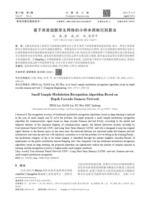
第47卷第4期Vol.47No.4计算机工程Computer Engineering2021年4月April 2021基于深度级联孪生网络的小样本调制识别算法冯磊,蒋磊,许华,苟泽中(空军工程大学信息与导航学院,西安710077)摘要:为解决传统基于深度学习的调制识别算法在小样本条件下识别准确率较低的问题,提出一种基于深度级联孪生网络的通信信号小样本调制识别算法。
根据通信信号时序图的时空特性,设计由卷积神经网络和长短时记忆网络级联的特征提取模块将原始信号特征映射至特征空间,同时在孪生网络架构下对提取的特征进行距离度量并以相似性约束训练网络,避免特征提取模块在训练过程中出现过拟合现象,最终通过最近邻分类器识别待测样本的调制类别。
在DeepSig 公开调制数据集上的实验结果表明,与传统基于深度学习的调制识别算法相比,该算法能有效降低训练过程中所需的样本量,且在小样本条件下的识别准确率更高。
关键词:卷积神经网络;长短时记忆网络;孪生网络;小样本;调制识别开放科学(资源服务)标志码(OSID ):中文引用格式:冯磊,蒋磊,许华,等.基于深度级联孪生网络的小样本调制识别算法[J ].计算机工程,2021,47(4):108-114.英文引用格式:FENG Lei ,JIANG Lei ,XU Hua ,et al.Small sample modulation recognition algorithm based on depth cascade siamese network [J ].Computer Engineering ,2021,47(4):108-114.Small Sample Modulation Recognition Algorithm Based onDepth Cascade Siamese NetworkFENG Lei ,JIANG Lei ,XU Hua ,GOU Zezhong(Information and Navigation College ,Air Force Engineering University ,Xi ’an 710077,China )【Abstract 】The recognition accuracy of traditional modulation recognition algorithms based on deep learning is reducedin the case of small sample size.To solve the problem ,this paper proposes a small sample modulation recognition algorithm for communication signal based on deep cascade Siamese network.Firstly ,according to the spatial and temporal features of the sequence diagram of communication signals ,the feature extraction module cascaded by Convolutional Neural Network (CNN )and Long Short Term Memory (LSTM )network is designed to map the original signal features to the feature space.At the same time ,the extracted features are measured under the Siamese network architecture ,and train the network with similarity constraints to avoid the problem of over fitting in the training.Finally ,the modulation category of the to be tested samples is identified through the nearest neighbor classifier.Results of experiments on the public modulation dataset DeepSig show that compared with the traditional modulation recognition algorithms based on deep learning ,the proposed algorithm can significantly reduce the number of samples required in training ,and the recognition accuracy is higher under small sample conditions.【Key words 】Convolutional Neural Network (CNN );Long Short Term Memory (LSTM )network ;Siamese network ;small sample ;modulation recognition DOI :10.19678/j.issn.1000-3428.00584720概述自从2012年Hinton 团队的深度卷积神经网络AlexNet 在ImageNet 挑战赛上获得冠军后[1],深度学习技术得到快速发展,各种针对语音识别和图像分类任务的新型深度网络被不断提出并取得了很好的处理效果,而基于深度学习技术的通信信号调制识别方法也成为当前国内外的研究热点。
常用的深度学习模型深度学习是一种涉及人工神经网络的机器学习方法,主要用于处理大型数据集,使模型能够更准确地预测和分类数据。
它已成为人工智能领域的一个热点,在计算机视觉、语音识别、自然语言处理等众多领域有广泛的应用。
本文将介绍常用的深度学习模型。
一、前馈神经网络(Feedforward Neural Network)前馈神经网络是最简单和最基本的深度学习模型,也是其他深度学习模型的基础。
它由输入层、隐藏层和输出层组成。
每层都由若干个神经元节点组成,节点与上一层或下一层的所有节点相连,并带有权重值。
前馈神经网络使用反向传播算法来训练模型,使它能够预测未来的数据。
二、卷积神经网络(Convolutional Neural Network)卷积神经网络是一种用于图像处理的深度学习模型,它能够对图像进行分类、分割、定位等任务。
它的核心是卷积层和池化层。
卷积层通过滤波器来识别图像中的特征,池化层则用于下采样,以减少计算量,同时保留重要特征。
卷积神经网络具有良好的特征提取能力和空间不变性。
三、递归神经网络(Recurrent Neural Network)递归神经网络是一种用于序列数据处理的深度学习模型,它能够处理可变长度的数据,如语音识别、自然语言处理等任务。
它的核心是循环层,每个循环层都可以接受来自上一次迭代的输出,并将其传递到下一次迭代。
递归神经网络具有记忆能力,能够学习序列数据的上下文信息。
四、长短时记忆网络(Long Short-Term Memory)长短时记忆网络是一种改进的递归神经网络,它能够处理长序列数据,并避免传统递归神经网络的梯度消失问题。
它的核心是LSTM单元,每个LSTM单元由输入门、遗忘门和输出门组成,能够掌握序列数据的长期依赖关系。
五、生成对抗网络(Generative Adversarial Networks)生成对抗网络是一种概率模型,由生成器和判别器两部分组成。
生成器用于生成假数据,判别器则用于将假数据与真实数据进行区分。

·技术前沿·航天电子对抗2021年第1期基于深度学习的雷达辐射源识别算法殷雪凤,武斌(西安电子科技大学电子工程学院,陕西西安710126)摘要:为解决雷达辐射源识别中特征提取困难、低信噪比条件下识别效率低的问题,提出了一种基于一维卷积神经网络和长短期记忆网络的深度学习智能识别算法,构建了一个CNN‑LSTM网络,能实现对不同脉内调制方式雷达辐射源的端到端识别。
该网络首先利用卷积层学习信号局部特征,然后将卷积层输出的结果输入长短期记忆网络,学习信号的全局特征,最终构造逻辑回归分类完成分类识别任务。
仿真结果表明,该算法较单一卷积神经网络模型具有更好的识别效果,抗噪声效果更强,在-6dB信噪比的条件下,识别的准确率仍能够达到90%以上。
关键词:卷积神经网络;长短期记忆网络;雷达辐射源识别;深度学习中图分类号:TN971+.5;TN974文献标志码:ARadar emitter identification algorithm based on deep learningYin Xuefeng,Wu Bin(School of Electronic Engineering,Xidian University,Xi’an710126,Shanxi,China)Abstract:In order to solve problems of feature extraction and low recognition efficiency under low signal-to-noise ratio in radar emitter identification,a deep learning intelligent recognition algorithm is proposed based onone-dimensional convolutional neural network and long short-term memory(CNN-LSTM)network.A CNN-LSTM network is constructed,which can realize end-to-end identification of different pulse modulation radarsources.The convolutional layers are used to learn the local characteristics of the signal by this network,and thelong short-term memory layer is used to learn the global characteristics.Finally a logistic regression classificationis constructed to complete the recognition task.Simulation results show that the algorithm has better recognitioneffect and stronger anti-noise effect compared with the single convolutional neural network model.Under the con‑dition of-6dB signal-to-noise ratio,the recognition accuracy can still reach more than90%.Key words:convolutional neural network;long short-term memory network;radar emitter identification;deep learning0引言雷达辐射源识别(REI/RER)技术是电子战中至关重要的一部分,是电子支援措施(ESM)的核心和雷达对抗系统中的关键技术[1]。
卷积神经网络在字符识别方面的应用一、概述二、背景三、人脑视觉机理四、关于特征4.1、特征表示的粒度4.2、初级(浅层)特征表示4.3、结构性特征表示4.4、需要有多少个特征, 五、Deep Learning的基本思想六、浅层学习(Shallow Learning)和深度学习(Deep Learning)七、Deep learning与Neural Network 八、Deep learning训练过程8.1、传统神经网络的训练方法8.2、deep learning训练过程九、Deep Learning的常用模型或者方法9.1、AutoEncoder自动编码器9.2、Sparse Coding稀疏编码9.3、Restricted Boltzmann Machine(RBM)限制波尔兹曼机9.4、Deep BeliefNetworks深信度网络9.5、Convolutional Neural Networks卷积神经网络十、总结与展望十一、参考文献和Deep Learning学习资源一、概述Artificial Intelligence,也就是人工智能,就像长生不老和星际漫游一样,是人类最美好的梦想之一。
虽然计算机技术已经取得了长足的进步,但是到目前为止,还没有一台电脑能产生“自我”的意识。
是的,在人类和大量现成数据的帮助下,电脑可以表现的十分强大,但是离开了这两者,它甚至都不能分辨一个喵星人和一个汪星人。
图灵(图灵,大家都知道吧。
计算机和人工智能的鼻祖,分别对应于其著名的“图灵机”和“图灵测试”)在 1950 年的论文里,提出图灵试验的设想,即,隔墙对话,你将不知道与你谈话的,是人还是电脑。
这无疑给计算机,尤其是人工智能,预设了一个很高的期望值。
但是半个世纪过去了,人工智能的进展,远远没有达到图灵试验的标准。
这不仅让多年翘首以待的人们,心灰意冷,认为人工智能是忽悠,相关领域是“伪科学”。
但是自 2006 年以来,机器学习领域,取得了突破性的进展。
Convolutional Neural Networks卷积神经网络卷积神经网络是人工神经网络的一种,已成为当前语音分析和图像识别领域的研究热点。
它的权值共享网络结构使之更类似于生物神经网络,降低了网络模型的复杂度,减少了权值的数量。
该优点在网络的输入是多维图像时表现的更为明显,使图像可以直接作为网络的输入,避免了传统识别算法中复杂的特征提取和数据重建过程。
卷积网络是为识别二维形状而特殊设计的一个多层感知器,这种网络结构对平移、比例缩放、倾斜或者共他形式的变形具有高度不变性。
CNNs是受早期的延时神经网络(TDNN)的影响。
延时神经网络通过在时间维度上共享权值降低学习复杂度,适用于语音和时间序列信号的处理。
CNNs是第一个真正成功训练多层网络结构的学习算法。
它利用空间关系减少需要学习的参数数目以提高一般前向BP算法的训练性能。
CNNs作为一个深度学习架构提出是为了最小化数据的预处理要求。
在CNN中,图像的一小部分(局部感受区域)作为层级结构的最低层的输入,信息再依次传输到不同的层,每层通过一个数字滤波器去获得观测数据的最显著的特征。
这个方法能够获取对平移、缩放和旋转不变的观测数据的显著特征,因为图像的局部感受区域允许神经元或者处理单元可以访问到最基础的特征,例如定向边缘或者角点。
2)卷积神经网络的网络结构图:卷积神经网络的概念示范:输入图像通过和三个可训练的滤波器和可加偏置进行卷积,滤波过程如图一,卷积后在C1层产生三个特征映射图,然后特征映射图中每组的四个像素再进行求和,加权值,加偏置,通过一个Sigmoid函数得到三个S2层的特征映射图。
这些映射图再进过滤波得到C3层。
这个层级结构再和S2一样产生S4。
最终,这些像素值被光栅化,并连接成一个向量输入到传统的神经网络,得到输出。
一般地,C层为特征提取层,每个神经元的输入与前一层的局部感受野相连,并提取该局部的特征,一旦该局部特征被提取后,它与其他特征间的位置关系也随之确定下来;S层是特征映射层,网络的每个计算层由多个特征映射组成,每个特征映射为一个平面,平面上所有神经元的权值相等。
长短期记忆网络在自然语言处理中的应用长短期记忆网络(Long Short-Term Memory, LSTM)是一种神经网络模型,它的出现解决了传统的RNN(Recurrent Neural Network)模型无法处理长序列数据的问题。
在自然语言处理中,LSTM具有极高的应用价值,可以用于文本分类、命名实体识别、机器翻译等任务。
本文将探讨LSTM在自然语言处理中的应用。
一、LSTM的基本原理LSTM的基本模型由一个单位(unit)和记忆细胞(memory cell)组成。
记忆细胞是LSTM的核心,其中包含了一些门(gates)来控制信息的流入与流出。
LSTM的门有三种:输入门(input gate)、遗忘门(forget gate)和输出门(output gate)。
输入门:用于控制新信息的流入。
在每个时间步上,输入门会根据当前输入和上一个时间步的隐藏状态计算出一个0-1之间的权重向量。
这个向量将控制哪些信息会进入到当前的记忆细胞中。
遗忘门:用于控制旧信息的保留。
在每个时间步上,遗忘门会根据当前的输入和上一个时间步的隐藏状态计算出一个0-1之间的权重向量。
这个向量将指定哪些信息从上一个记忆细胞中被保留下来,并传递到当前的记忆细胞中。
输出门:用于控制记忆细胞中哪些信息将被用作当前时间步的输出。
在每个时间步上,输出门会根据当前的输入和隐藏状态计算出一个0-1之间的权重向量。
这个向量将筛选出记忆细胞中需要输出的信息。
通过这些门的控制,LSTM能够有效地处理长序列数据,避免了传统的RNN模型中存在的梯度消失和爆炸的问题。
二、LSTM在文本分类中的应用文本分类是NLP中最基本的任务之一,它的目标是将一些文本分类到预定义的类别之中。
LSTM的输入是一个词向量序列,输出是表示输入文本分类的向量。
在LSTM中,输入序列中的每个词向量都会被传递到一个LSTM单位中。
每个LSTM单位将根据它之前和它接收到的输入计算出一个隐藏状态并输出到下一个LSTM单位。
convlstm分类ConvLSTM分类是一种集成了卷积神经网络(Convolutional Neural Network,CNN)和长短期记忆网络(Long Short-Term Memory,LSTM)的神经网络分类方法。
它通常被用于处理视频(包括动态图像和连续帧)等序列数据,将时间维度加入到CNN分类中,从而可以更好地对序列数据进行处理和分类。
接下来,我们将分步骤阐述ConvLSTM分类方法。
第一步:卷积神经网络卷积神经网络(CNN)是一种常用的深度学习算法,在图像分类、目标检测等领域都具有优秀的表现。
对于图像分类问题,CNN通过多个卷积层提取图像特征,再通过全连接层进行分类。
其中,卷积层可以提取局部特征,全连接层可以学习到全局特征。
第二步:长短期记忆网络长短期记忆网络(LSTM)是一种适用于序列数据处理的神经网络。
相较于传统的循环神经网络(Recurrent Neural Network,RNN),LSTM可以更好地处理长序列、避免梯度消失/梯度爆炸等问题。
在LSTM中,每个单元内部包含输出门(Output Gate)、输入门(Input Gate)、遗忘门(Forget Gate)和细胞状态(Cell State),可以同时学习到序列中当前状态和历史状态的信息。
第三步:ConvLSTMConvLSTM是Convolutional LSTM的缩写,是一种结合了CNN和LSTM的网络结构,可以在对序列数据进行处理的同时利用卷积提取空间信息。
ConvLSTM的主要思想是将LSTM单元替换成卷积核,通过卷积操作实现对序列数据的处理。
此外,ConvLSTM还可以通过交替堆叠多个ConvLSTM层来增加模型深度,提高分类性能。
第四步:ConvLSTM分类ConvLSTM分类是将ConvLSTM应用于序列分类任务的方法。
在ConvLSTM分类任务中,通过将原始数据划分为训练集和测试集,对训练集进行训练,对测试集进行测试,最终得到对序列数据进行分类的准确性评估。
深度学习中的循环神经网络训练技巧分享循环神经网络(Recurrent Neural Networks,RNN)是一种在深度学习中广泛应用的模型,用于处理序列数据,例如语音识别、自然语言处理和时间序列预测等任务。
然而,由于RNN模型的复杂性和长期依赖问题,有效地训练RNN模型一直是一个具有挑战性的任务。
在本文中,我们将分享一些深度学习中的循环神经网络训练技巧,帮助读者克服一些常见的训练困难。
1. 梯度剪裁(Gradient Clipping)由于RNN模型中存在长期依赖的问题,训练过程中可能出现梯度爆炸的情况,导致模型无法正确学习。
为了解决这个问题,可以采用梯度剪裁技术。
梯度剪裁通过设置一个梯度阈值,当梯度的范数超过该阈值时,将梯度按比例缩放,以防止梯度爆炸的问题。
这个技巧可以提高模型的稳定性和收敛速度。
2. 逆序输入(Reverse Input)在处理序列数据时,逆序输入的技巧可以帮助模型更好地捕捉到长期依赖关系。
传统的RNN模型处理序列数据时往往是按照时间顺序依次输入,而逆序输入则是将序列数据进行逆序处理,让模型首先获取到序列的后面部分,有助于提高模型对序列结构的理解能力。
3. 双向RNN(Bidirectional RNN)双向RNN是一种使用两个相互独立的RNN模型来处理序列数据的方法。
其中一个RNN按照正向顺序处理序列数据,另一个RNN按照逆向顺序处理序列数据,最后将两个RNN的输出进行合并,以获得更全面的序列信息。
双向RNN可以更好地捕捉到序列数据中的上下文信息,提高模型的性能。
4. 注意力机制(Attention Mechanism)注意力机制是一种让模型自动关注输入序列中重要部分的技巧。
传统的RNN模型在处理长序列时,可能会忽略一些重要的上下文信息,导致性能下降。
通过引入注意力机制,模型可以根据当前的状态自动选择输入序列中有用的信息进行处理,提高模型对序列数据的理解能力。
注意力机制在机器翻译和文本摘要等任务中取得了显著的性能提升。
cv相关算法模型计算机视觉(Computer Vision,简称CV)是人工智能领域的一个重要分支,致力于让计算机具备感知和理解图像或视频的能力。
在CV相关算法模型中,有许多经典的算法和模型被广泛应用于图像处理、目标检测、图像分割等领域。
本文将介绍几个常见的CV算法模型,并探讨其应用和优缺点。
一、卷积神经网络(Convolutional Neural Networks,简称CNN)卷积神经网络是一种深度学习模型,模拟了人类视觉系统的工作原理,通过多层卷积和池化操作提取图像特征,并通过全连接层进行分类。
CNN在图像分类、目标检测和图像分割等任务上取得了显著的成果。
然而,CNN在处理大规模数据和复杂背景下的性能仍有待提高。
二、循环神经网络(Recurrent Neural Networks,简称RNN)循环神经网络是一种具有记忆功能的神经网络,通过将当前输入和前一时刻的输出进行循环计算,可以处理序列数据。
在CV领域,RNN常用于图像描述生成、视频分析等任务。
然而,由于RNN的计算过程是串行的,导致其在处理长序列时容易出现梯度消失或梯度爆炸的问题。
三、生成对抗网络(Generative Adversarial Networks,简称GAN)生成对抗网络由生成器和判别器两个模型组成,通过对抗学习的方式,使生成器生成的样本更加逼真。
GAN在图像生成、图像转换等任务上取得了很好的效果,如生成逼真的人脸图像、将草图转换为真实图像等。
然而,GAN的训练过程相对不稳定,容易出现模式崩溃和模式坍塌的问题。
四、目标检测算法模型目标检测是CV领域的一个重要任务,旨在从图像中准确地找出并定位出感兴趣的目标。
目前,一些主流的目标检测算法模型包括:基于区域的卷积神经网络(RCNN)、快速的RCNN(Fast RCNN)、更快的RCNN(Faster RCNN)和单阶段检测器(YOLO、SSD)。
这些模型在目标检测的准确性和速度上有不同的权衡。
人工智能之卷积神经网络人工智能之机器学习主要有三大类:1)分类;2)回归;3)聚类。
今天我们重点探讨一下卷积神经网络(CNN)算法。
前言:人工智能机器学习有关算法内容,请参见公众号“科技优化生活”之前相关文章。
人工智能之机器学习主要有三大类:1)分类;2)回归;3)聚类。
今天我们重点探讨一下卷积神经网络(CNN)算法。
20世纪60年代,Hubel和Wiesel在研究猫脑皮层中用于局部敏感和方向选择的神经元时发现其独特的网络结构可以有效地降低反馈神经网络的复杂性,继而提出了卷积神经网络CNN(Convolutional Neural Networks)。
1980年,K.Fukushima提出的新识别机是卷积神经网络的第一个实现网络。
随后,更多的科研工作者对该网络进行了改进。
其中,具有代表性的研究成果是Alexander和Taylor 提出的“改进认知机”,该方法综合了各种改进方法的优点并避免了耗时的误差反向传播。
现在,CNN已经成为众多科学领域的研究热点之一,特别是在模式分类领域,由于该网络避免了对图像的复杂前期预处理,可以直接输入原始图像,因而得到了更为广泛的应用。
CNN概念:在机器学习中,卷积神经网络CNN(Convolutional Neural Network)是一种前馈神经网络,它的人工神经元可以响应一部分覆盖范围内的周围单元,可以应用于语音识别、图像处理和图像识别等领域。
CNN引入意义:在全连接神经网络中(下面左图),每相邻两层之间的每个神经元之间都是有边相连的。
当输入层的特征维度变得很高时,这时全连接网络需要训练的参数就会增大很多,计算速度就会变得很慢。
而在卷积神经网络CNN中(下面右图),卷积层的神经元只与前一层的部分神经元节点相连,即它的神经元间的连接是非全连接的,且同一层中某些神经元之间的连接的权重w和。
机器学习技术中的循环神经网络模型介绍机器学习是一门研究如何使计算机可以自动进行学习的技术,而循环神经网络(Recurrent Neural Network,简称RNN)则是机器学习中的一种重要神经网络模型。
RNN模型具有记忆能力,可以处理序列数据,并且在语音识别、自然语言处理、机器翻译等领域取得了很多成果。
循环神经网络模型中最重要的特点是共享权重和循环连接。
共享权重意味着在模型的不同时间步骤中,相同位置的权重参数是共享的,这使得RNN可以有效地处理不定长的序列数据。
循环连接则使得当前时间步的输入不仅仅依赖于当前时刻的输入,还依赖于前一时刻的输出。
这种具有记忆性的结构使RNN能够在处理序列数据时考虑到各个时刻的上下文信息。
在循环神经网络模型中,最基本的结构是简单循环神经网络(Simple Recurrent Neural Network,简称SRNN)。
SRNN的基本单元是一个隐含层,通常使用tanh或sigmoid激活函数。
隐含层的输出会被作为下一个时间步的输入,这样隐含层的信息可以在不同的时间步骤中传递下去。
SRNN由于存在梯度消失或梯度爆炸的问题,难以处理长距离依赖的序列数据。
为了解决SRNN的问题,长短期记忆网络(Long Short-Term Memory,简称LSTM)被提出。
LSTM是一种特殊的RNN结构,通过引入门控单元和记忆单元,有效地解决了梯度消失和梯度爆炸问题。
LSTM模型能够更好地捕捉序列数据中的长期依赖关系。
LSTM中的关键组成部分是门控单元(Gate Cell),包括输入门(Input Gate)、遗忘门(Forget Gate)和输出门(Output Gate)。
输入门决定是否更新记忆单元的内容,遗忘门决定从记忆单元中遗忘哪些信息,输出门决定从记忆单元输出哪些信息。
这些门控单元通过一个非线性函数将输入、上一时间步的输出和记忆单元的内容综合起来,实现了对序列数据的灵活建模。
循环神经网络 RNN发展史概述循环神经网络(Recurrent Neural Network, RNN)是一类以序列(sequence)数据为输入,在序列的演进方向进行递归(recursion)且所有节点(循环单元)按链式连接的递归神经网络(recursive neural network)。
对循环神经网络的研究始于二十世纪80-90年代,并在二十一世纪初发展为深度学习(deep learning)算法之一,其中双向循环神经网络(Bidirectional RNN, Bi-RNN)和长短期记忆网络(Long Short-Term Memory networks,LSTM)是常见的循环神经网络。
1982年,美国加州理工学院物理学家John Hopfield发明了一种单层反馈神经网络Hopfield Network,用来解决组合优化问题。
这是最早的RNN的雏形。
86年,另一位机器学习的泰斗Michael I.Jordan 定义了Recurrent的概念,提出Jordan Network。
1990年,美国认知科学家Jeffrey L.Elman对Jordan Network进行了简化,并采用BP算法进行训练,便有了如今最简单的包含单个自连接节点的RNN模型。
但此时RNN由于梯度消失(Gradient Vanishing)及梯度爆炸(Gradient Exploding)的问题,训练非常困难,应用非常受限。
直到1997年,瑞士人工智能研究所的主任Jurgen Schmidhuber提出长短期记忆(LSTM),LSTM使用门控单元及记忆机制大大缓解了早期RNN训练的问题。
同样在1997年,Mike Schuster提出双向RNN模型(Bidirectional RNN)。
这两种模型大大改进了早期RNN结构,拓宽了RNN的应用范围,为后续序列建模的发展奠定了基础。
此时RNN虽然在一些序列建模任务上取得了不错的效果,但由于计算资源消耗大,后续几年一直没有太大的进展。
第42卷第9期自动化学报Vol.42,No.9 2016年9月ACTA AUTOMATICA SINICA September,2016图像理解中的卷积神经网络常亮1,2邓小明3周明全1,2武仲科1,2袁野3,4杨硕3,4王宏安3摘要近年来,卷积神经网络(Convolutional neural networks,CNN)已在图像理解领域得到了广泛的应用,引起了研究者的关注.特别是随着大规模图像数据的产生以及计算机硬件(特别是GPU)的飞速发展,卷积神经网络以及其改进方法在图像理解中取得了突破性的成果,引发了研究的热潮.本文综述了卷积神经网络在图像理解中的研究进展与典型应用.首先,阐述卷积神经网络的基础理论;然后,阐述其在图像理解的具体方面,如图像分类与物体检测、人脸识别和场景的语义分割等的研究进展与应用.关键词卷积神经网络,图像理解,深度学习,图像分类,物体检测引用格式常亮,邓小明,周明全,武仲科,袁野,杨硕,王宏安.图像理解中的卷积神经网络.自动化学报,2016,42(9): 1300−1312DOI10.16383/j.aas.2016.c150800Convolutional Neural Networks in Image Understanding CHANG Liang1,2DENG Xiao-Ming3ZHOU Ming-Quan1,2WU Zhong-Ke1,2YUAN Ye3,4YANG Shuo3,4WANG Hong-An3Abstract Convolutional neural networks(CNN)have been widely applied to image understanding,and they have arose much attention from researchers.Specifically,with the emergence of large image sets and the rapid development of GPUs, convolutional neural networks and their improvements have made breakthroughs in image understanding,bringing about wide applications into this area.This paper summarizes the up-to-date research and typical applications for convolutional neural networks in image understanding.Wefirstly review the theoretical basis,and then we present the recent advances and achievements in major areas of image understanding,such as image classification,object detection,face recognition, semantic image segmentation etc.Key words Convolutional neural networks(CNN),image understanding,deep learning,image classification,object detectionCitation Chang Liang,Deng Xiao-Ming,Zhou Ming-Quan,Wu Zhong-Ke,Yuan Ye,Yang Shuo,Wang Hong-An. Convolutional neural networks in image understanding.Acta Automatica Sinica,2016,42(9):1300−13121986年,Rumelhart等[1]提出人工神经网络的反向传播算法(Back propagation,BP),掀起了神经网络在机器学习中的研究热潮.神经网络中存在大量的参数,存在容易发生过拟合、训收稿日期2015-12-11录用日期2016-05-03Manuscript received December11,2015;accepted May3,2016国家自然科学基金(61402040,61473276),中国科学院青年创新促进会资助Supported by National Natural Science Foundation of China (61402040,61473276)and Youth Innovation Promotion Associ-ation,Chinese Academy of Sciences本文责任编委柯登峰Recommended by Associate Editor KE Deng-Feng1.北京师范大学信息科学与技术学院北京1008752.教育部虚拟现实应用工程研究中心北京1008753.中国科学院软件研究所人机交互北京市重点实验室北京1001904.中国科学院大学计算机与控制学院北京1000491.College of Information Science and Technology,Beijing Normal University,Beijing1008752.Engineering Research Center of Virtual Reality and Applications,Ministry of Educa-tion,Beijing1008753.Beijing Key Laboratory of Human-Computer Interactions,Institute of Software,Chinese Academy of Sciences,Beijing1001904.School of Computer and Control Engineering,University of Chinese Academy of Sciences,Beijing 100049练时间长的缺陷,但是与基于规则的学习相比已经具有优越性.基于统计学习理论的支持向量机[2]、Boosting、Logistic回归方法可以被看作具有一层隐节点或者不含隐节点的学习模型,被称为浅层机器学习模型.浅层学习模型通常需要由人工方法获取好的样本特征,在此基础上进行识别和预测,因此方法的有效性很大程度上受到特征提取的制约[3].2006年,Hinton等[4]在Science上提出了深度学习.这篇文章的两个主要观点是:1)多隐层的人工神经网络具有优异的特征学习能力,学习到的数据更能反映数据的本质特征,有利于可视化或分类;2)深度神经网络在训练上的难度,可以通过逐层无监督训练有效克服.理论研究表明为了学习到可表示高层抽象特征的复杂函数,需要设计深度结构.深度结构由多层非线性算子构成,典型设计是具有多层隐节点的神经网络.随着网络层数的加大,如何搜索深度结构的参数空间成为具有挑战性的任务.近年来,深度学习取得成功的主要原因有:1)在训练9期常亮等:图像理解中的卷积神经网络1301数据上,大规模训练数据的出现(如ImageNet[5]),为深度学习提供了好的训练资源;2)计算机硬件的飞速发展(特别是GPU的出现)使得训练大规模神经网络成为可能.与浅层学习模型相比,深度学习构造了具有多隐层的学习模型,设计了有效的学习算法并能够加速计算,从而能够对大数据进行处理;通过深度学习能够得到更高层的特征,从而提高样本的识别率或预测的准确率.卷积神经网络(Convolutional neural net-works,CNN)是一种带有卷积结构的深度神经网络,卷积结构可以减少深层网络占用的内存量,也可以减少网络的参数个数,缓解模型的过拟合问题. 1989年,LeCun等[6]在手写数字识别中采用神经网络误差反向传播算法,在网络结构设计中加入下采样(Undersampling)与权值共享(Weight shar-ing).1998年,LeCun等[7]提出用于文档识别的卷积神经网络,为了保证一定程度的平移、尺度、畸变不变性,CNN设计了局部感受野、共享权重和空间或时间下采样,提出用于字符识别的卷积神经网络LeNet-5.LeNet-5由卷积层、下采样层、全连接层构成,该系统在小规模手写数字识别中取得了较好的结果.2012年,Krizhevsky等[8]采用称为AlexNet的CNN在ImageNet竞赛图像分类任务中取得了最好的成绩,是CNN在大规模图像分类中的巨大成功.AlexNet网络具有更深层的结构,并设计了ReLU(Rectified linear unit)作为非线性激活函数以及Dropout来避免过拟合.在图像分类中,一个重要的图像数据库是ImageNet[5].针对具有80000个同义词的词汇网络(WordNet),ImageNet 旨在分别使用500∼1000个清晰的全分辨率图像来表示其中的大部分词汇,这样就形成了上百万张有标记的图像,它们通过词汇网络的语义结构组织起来.ImageNet总共包括12个子树、5247个同义词集、320万图像,是目标检测、图像分类、图像定位研究的优越资源,ImageNet在大规模、准确度、分层结构方面为计算机视觉研究者提供了前所未有的机会.表1是ImageNet竞赛历年来图像分类任务的部分领先结果.在AlexNet之后,研究者又进一步改善网络性能,提出能有效分类检测的R-CNN(Region-based CNN)[9]、SPP(Spatial pyra-mid pooling)-net[10]、GoogLeNet[11]、VGG(Visual geometry group)[12]等.为了更好地改进卷积神经网络,使其在应用中发挥更大的功效,研究者不仅从应用的特殊性、网络的结构等方面进一步探讨卷积神经网络,而且从其中的网络层设计、损失函数的设计、激活函数、正则项等多方面对现有网络进行改进,取得了一系列成果.计算机视觉的中心任务就是通过对图像或图像序列的分析,得到景物的尽可能完全正确的描述[13].图像理解与计算机视觉紧密相关,研究内容交叉重合,图像理解侧重在图像分析的基础上,理解图像内容的含义以及解释原来的客观场景,从而指导和规划行动[14].图像理解是深度学习应用最早的领域,也是其应用最广的领域之一.随着互联网大数据的兴起,深度学习在大规模图像的处理中显示了不可替代的优越性.卷积神经网络的研究已经在图像理解中广泛应用[3].本文着重阐述卷积神经网络的理论和面向图像理解几个不同方面的卷积神经网络的提出、进展和应用,包括:图像分类和物体检测、人脸识别和验证、场景的语义分割和深度恢复、人体关节检测,通过这些介绍希望能帮助读者了解相关工作的方法和思路并启发新的研究思路.表1ImageNet竞赛历年来图像分类任务的部分领先结果Table1Representative top ranked results in imageclassification task of“ImageNet Large Scale VisualRecognition Challenge”公布时间机构Top-5错误率(%)2015.12.10MSRA 3.57[15]2014.8.18Google 6.66[11]2014.8.18Oxford7.33[12]2013.11.14NYU11.72012.10.13U.Toronto16.4[8]1卷积神经网络卷积神经网络是深度学习的一种,已成为当前图像理解领域的研究热点[6,16−17]它的权值共享网络结构使之更类似于生物神经网络,降低了网络模型的复杂度,减少了权值的数量.这个优点在网络的输入是多维图像时表现得更为明显,图像可以直接作为网络的输入,避免了传统识别算法中复杂的特征提取和数据重建过程.卷积网络是为识别二维形状而特殊设计的一个多层感知器,这种网络结构对平移、比例缩放以及其他形式的变形具有一定不变性.在典型的CNN中,开始几层通常是卷积层和下采样层的交替,在靠近输出层的最后几层网络通常是全连接网络(如图1所示).卷积神经网络的训练过程主要是学习卷积层的卷积核参数和层间连接权重等网络参数,预测过程主要是基于输入图像和网络参数计算类别标签.卷积神经网络的关键是:网络结构(含卷积层、下采样层、全连接层等)和反向传播算法等.在本节中,我们先介绍典型CNN的网络结构和反向传播算法,然后概述常用的其他CNN网络结构和方法.神经网络参数的中文名称主要参考文献[18]卷积神经网络的结构和反向传播算法主要参考文献[17].1302自动化学报42卷图1卷积神经网络示例Fig.1Illustration of convolutional neural networks1.1网络结构1.1.1卷积层在卷积层,上一层的特征图(Feature map)被一个可学习的卷积核进行卷积,然后通过一个激活函数(Activation function),就可以得到输出特征图.每个输出特征图可以组合卷积多个特征图的值[17]:x l j =f(u lj)u l j =i∈M jx l−1i∗k lij+b lj(1)其中,u l j称为卷积层l的第j个通道的净激活(Net activation),它通过对前一层输出特征图x l−1i进行卷积求和与偏置后得到的,x l j是卷积层l的第j个通道的输出.f(·)称为激活函数,通常可使用sig-moid和tanh等函数.M j表示用于计算u lj的输入特征图子集,k l ij是卷积核矩阵,b l j是对卷积后特征图的偏置.对于一个输出特征图x l j,每个输入特征图x l−1i对应的卷积核k l ij可能不同,“*”是卷积符号.1.1.2下采样层下采样层将每个输入特征图通过下面的公式下采样输出特征图[17]:x l j =f(u lj)u l j =βljdown(x l−1j)+b lj(2)其中,u l j称为下采样层l的第j通道的净激活,它由前一层输出特征图x l−1i进行下采样加权、偏置后得到,β是下采样层的权重系数,b l j是下采样层的偏置项.符号down(·)表示下采样函数,它通过对输入特征图x l−1j通过滑动窗口方法划分为多个不重叠的n×n图像块,然后对每个图像块内的像素求和、求均值或最大值,于是输出图像在两个维度上都缩小了n倍.1.1.3全连接层在全连接网络中,将所有二维图像的特征图拼接为一维特征作为全连接网络的输入.全连接层l 的输出可通过对输入加权求和并通过激活函数的响应得到[17]:x l=f(u l)u l=w l x l−1+b l (3)其中,u l称为全连接层l的净激活,它由前一层输出特征图x l−1进行加权和偏置后得到的.w l是全连接网络的权重系数,b l是全连接层l的偏置项.1.2反向传播算法神经网络有两类基本运算模式:前向传播和学习.前向传播是指输入信号通过前一节中一个或多个网络层之间传递信号,然后在输出层得到输出的过程.反向传播算法是神经网络有监督学习中的一种常用方法,其目标是根据训练样本和期望输出来估计网络参数.对于卷积神经网络而言,主要优化卷积核参数k、下采样层网络权重β、全连接层网络权重w和各层的偏置参数b等.反向传播算法的本质在于允许我们对每个网络层计算有效误差,并由此推导出一个网络参数的学习规则,使得实际网络输出更加接近目标值[18].我们以平方误差损失函数的多分类问题为例介绍反向传播算法的思路.考虑一个多分类问题的训练总误差,定义为输出端的期望输出值和实际输出值的差的平方[17]:E(w,β,k,b)=12Nn=1t n−y n 2(4)其中,t n是第n个样本的类别标签真值,y n是第n个样本通过前向传播网络预测输出的类别标签.对于多分类问题,输出类别标签常用一维向量表示,即输入样本对应的类别标签维度为正数,输出类别标签的其他维为0或负数,这取决于选择的激活函数类型,当激活函数选为sigmoid,输出标签为0,当激活函数为tanh,输出标签为−1.反向传播算法主要基于梯度下降方法,网络参数首先被初始化为随机值,然后通过梯度下降法向训练误差减小的方向调整.接下来,我们以多个“卷积层–采样层”连接多个全连接层的卷积神经网络为例介绍反向传播算法.首先介绍网络第l层的灵敏度(Sensitiv-ity)[17−18]:δl=∂E∂u l(5)其中,δl描述了总误差E怎样随着净激活u l而变化.反向传播算法实际上通过所有网络层的灵敏度9期常亮等:图像理解中的卷积神经网络1303建立总误差对所有网络参数的偏导数,从而得到使得训练误差减小的方向.1.2.1卷积层为计算卷积层l的灵敏度,需要用下一层下采样层l+1的灵敏度表示卷积层l的灵敏度,然后计算总误差E对卷积层参数(卷积核参数k、偏置参数b)的偏导数.由于下采样层的灵敏度尺寸小于卷积层的灵敏度尺寸,因此需要将下采样层l+1的灵敏度上采样到卷积层l的灵敏度大小,然后将第l层净激活的激活函数偏导与从第l+1层的上采样得到的灵敏度逐项相乘.分别由式(1)和(2),通过链式求导可得第l层中第j个通道的灵敏度[17]:δl j =∂E∂u lj=βl+1j(f (u lj)◦up(δl+1j))(6)其中,up(·)表示一个上采样操作,符号◦表示每个元素相乘.若下采样因子为n,则up(·)将每个像素在水平和垂直方向上复制n次,于是就可以从l+1层的灵敏度上采样成卷积层l的灵敏度大小.函数up(·)可以用Kronecker乘积up(x)≡x⊗1n×n来实现.然后,使用灵敏度对卷积层l中的参数计算偏导.对于总误差E对偏移量b l j的偏导,可以对卷积层l的灵敏度中所有节点进行求和来计算:∂E ∂b lj =u,v(δlj)u,v(7)对于总误差关于卷积核参数的偏导,由式(1),使用链式求导时需要用所有与该卷积核相乘的特征图元素来求偏导:∂E ∂k lij =u,v(δlj)u,v(p l−1i)u,v(8)其中,(p l−1i )u,v是在计算x lj时,与k l ij逐元素相乘的x l−1i元素.1.2.2下采样层为计算下采样层l的灵敏度,需要用下一层卷积层l+1的灵敏度表示下采样层l的灵敏度,然后计算总误差E对下采样参数权重系数β、偏置参数b的偏导数.为计算我们需要下采样层l的灵敏度,我们必须找到当前层的灵敏度与下一层的灵敏度的对应点,这样才能对灵敏度δ进行递推.另外,需要乘以输入特征图与输出特征图之间的连接权值,这个权值实际上就是卷积核的参数.分别由式(1)和(2),通过链式求导可得第l层第j个通道的灵敏度[17]:δl j =f (u lj)◦conv2(δl+1j,rot180(k l+1j) ,full )(9)其中,对卷积核旋转180度使用卷积函数计算互相关(在Matlab中,可用conv2函数实现),对卷积边界进行补零处理.然后,总误差对偏移量b的偏导与前面卷积层的一样,只要对灵敏度中所有元素的灵敏度求和即可:∂E∂b lj=u,v(δlj)u,v(10)对于下采样权重β,我们先定义下采样算子d lj=down(x l−1j),然后可通过下面的公式计算总误差E对β的偏导:∂E∂βlj=u,v(δlj◦d lj)u,v(11)这里我们假定下采样层的下一层为卷积层,如果下一层为全连接层,也可以做类似的推导.1.2.3全连接层全连接层l的灵敏度可通过下式计算:δl=(w l+1)Tδl+1◦f (u l)(12)输出层的神经元灵敏度可由下面的公式计算:δL=f (u L)◦(y n−t n)(13)总误差对偏移项的偏导如下:∂E∂b l=∂E∂u l∂u l∂b l=δl(14)接下来可以对每个神经元运用灵敏度进行权值更新.对一个给定的全连接层l,权值更新方向可用该层的输入x l−1和灵敏度δl的内积来表示:∂E∂w l=x l−1(δl)T(15)1.2.4网络参数更新过程卷积层参数可用下式更新:∆k lij=−η∂E∂k lij(16)∆b l=−η∂E∂b l(17)下采样层参数可用下式更新:∆βl=−η∂E∂βl(18)∆b l=−η∂E∂b l(19)全连接层参数可用下式更新:∆w l=−η∂E∂w l(20)1304自动化学报42卷其中,对于每个网络参数都有一个特定的学习率η.若学习率太小,则训练的速度慢;若学习率太大,则可导致系统发散.在实际问题中,如果总误差在学习过程中发散,那么将学习率调小;反之,如果学习速度过慢,那么将学习率调大.1.3常用的其他网络结构和方法1.3.1卷积层传统卷积神经网络的卷积层采用线性滤波器与非线性激活函数,一种改进的方法在卷积层使用多层感知机模型作为微型神经网络,通过在输入图像中滑动微型神经网络来得到特征图,该方法能够增加神经网络的表示能力,被称为Network in net-work[19].为了解决既能够保证网络的稀疏性,又能够利用稠密矩阵的高性能计算,Szegedy等[11]提出Inception网络.Inception网络的一层含有一个池化操作和三类卷积操作:1×1、3×3、5×5卷积.1.3.2池化池化(Pooling)是卷积神经网络中一个重要的操作,它能够使特征减少,同时保持特征的局部不变性.常用的池化操作有:空间金字塔池化(Spatial pyramid pooling,SPP)[10]、最大池化(Max pooling)、平均池化(Mean pooling)、随机池化(Stochastic pooling)[20]等.本文第1.1.2节介绍的下采样层实际上也属于池化.1.3.3激活函数常用激活函数有:ReLU[8]、Leakly ReLU[21]、Parametric ReLU、Randomized ReLU、ELU等.1.3.4损失函数损失函数的选择在卷积神经网络中起重要作用,代表性的损失函数有:平方误差损失、互熵损失(Cross entropy loss)、Hinge损失等.1.3.5优化方法和技巧卷积神经网络常用的优化方法包含随机梯度下降方法(Stochastic gradient descent,SGD),常用的技巧有权值初始化[8]、权值衰减(Weight de-cay)[18]、Batch normalization[22]等.1.4卷积神经网络的优势卷积神经网络在下采样层可以保持一定局部平移不变形,在卷积层通过感受野和权值共享减少了神经网络需要训练的参数的个数.每个神经元只需要感受局部的图像区域,在更高层将这些感受不同局部区域的神经元综合起来就可以得到全局的信息.因此,可以减少网络连接的数目,即减少神经网络需要训练的权值参数的个数.由于同一特征通道上的神经元权值相同,所以网络可以并行学习,这也是卷积网络相对于神经元彼此相连网络的一大优势.卷积神经网络以其权值共享的特殊结构在图像理解领域中有着独特的优越性,通过权值共享降低了网络的复杂性.总之,卷积神经网络相比于一般神经网络在图像理解中有其特殊的优点:1)网络结构能较好适应图像的结构;2)同时进行特征提取和分类,使得特征提取有助于特征分类;3)权值共享可以减少网络的训练参数,使得神经网络结构变得更简单、适应性更强.2卷积神经网络在图像理解中的进展与应用本节将介绍卷积神经网络在图像分类与物体检测、人脸识别和验证、语义图像分割等方面的进展与应用.2.1图像分类和物体检测图像分类和物体检测是图像理解中的核心问题之一.图像分类是指给定图像,对图像的类别进行预测;物体检测是指对于图像中的同一物体或者同一类别物体进行检测,找到可能出现物体的区域.在图像分类和物体检测中,传统的方法包含基于词袋(Bag of words,BOW)的方法和基于变形模板模型(Deformable part models,DPM)[23]的方法等.这些方法虽然在某些特定应用(如人脸检测、行人检测等)中取得了很好的效果,但在准确性方面仍存在较大提升空间.随着深度学习的兴起,人们将深度学习应用于图像分类和物体检测问题中,并在许多应用中取得明显好于传统方法的结果.在图像分类中,Krizhevsky等[8]提出了新型卷积神经网络结构(AlexNet),GoogLeNet[11]和VGG[12]通过加深网络层数同时保证优化性能,设计了更深层次的卷积神经网络.在物体检测中,研究者使用区域选择性搜索[9]等技术提升检测的准确率,通过加入感兴趣区域池化层(Region of interest(ROI)pooling layer)[24]和空间金字塔池化[10]等技术加速网络计算速度.此外,也有一部分工作将卷积神经网络特征与传统视觉识别模型结合起来.Girshick等[25]利用深度学习的特征代替原有人工设计的方向梯度直方图(Histogram of oriented gradient,HOG)特征[26]建立变形模板,提升了传统变形模板方法(DPM)的识别率,并且在取得了与完全使用深度学习方法可比结果的同时,提升了检测速度.表2给出部分具有代表性的图像分类和物体检测模型对比.接下来,我们分别介绍面向图像分类和物体检测任务的AlexNet及代表性的改进方法、其他代表性的改进方向.2.1.1AlexNet及代表性的改进方法Krizhevsky等[8]提出新型卷积神经网络结构(简称为AlexNet,其网络结构如图2所示),并在9期常亮等:图像理解中的卷积神经网络1305图2AlexNet 卷积神经网络结构示意图[8]Fig.2Network architecture of AlexNet convolutional neural networks [8]ImageNet ILSVRC-2012图像分类问题中取得最好成绩(Top-5错误率为15.3%),其结果明显好于使用传统方法的第二名取得的结果(Top-5错误率为26.2%).该方法训练了一个端对端(End to end)的卷积神经网络实现图像特征提取和分类,网络结构共7层,包含5层卷积层和2层全连接层.AlexNet 在训练阶段使用了Dropout 技巧,并通过图像平移、图像水平翻转、调整图像灰度等方法扩充训练数据集,后者一方面通过扩充样本缓解了神经网络的过拟合以及对网络参数优化时陷入局部最优的问题,也使得训练得到的网络对局部平移和光照变化具有一定的不变性.为了加快网络训练的速度,AlexNet 采用ReLU 代替传统神经网络常用的激活函数tanh/sigmod,ReLU 是一种非饱和非线性(Non-saturating nonlinearity)变换.Overfeat [27]首次使用同一个模型完成图像分类、定位和物体检测三个任务,其主要观点是通过共享部分网络完成这三个任务,能相互促进每个任务的结果.Overfeat 继承了AlexNet 的网络结构,主要区别在于:AlexNet 在提出时主要面向图像分类任务,Overfeat 可以完成图像分类、定位和物体检测三个任务;Overfeat 在训练时输入固定大小的图像,测试时用多尺度输入,没有使用AlexNet 中的对比度归一化,采用无重叠区域的最大池化,前两层的特征图更大.对于分类与检测问题,常采用滑动窗口对每一个图像块进行检测,从而确定目标物体的类别与位置,即都需要一个滑动窗口对整幅图像进行密集采样.为提高计算效率,Overfeat 舍弃在图像层级的滑动,转而在特征层级进行滑动,明显减少了滑动窗口个数.为了避免特征层级采样带来的稀疏问题,Overfeat 采用多次采样插值的方法解决.对于图像分类、定位和物体检测问题的统一,Overfeat 采用复用权重的方式,即在每一个尺度上同时运行分类网络和定位回归网络.对于每一个尺度,分类网络给出了图像块的类别概率分布,回归网络进一步为每一类给出了包围盒和置信度.最后,综合这些信息,给出分类与检测结果.Overfeat 虽然提出了将分类、定位、检测任务一起解决的思想,但这三个任务在训练阶段仍是分开进行的[24].AlexNet 用于物体检测时,需要在图像金字塔上采用滑动窗口的方式逐个判断,随着图像的增大待检测区域的数目呈平方上升.为了解决这一问题,Girshick 等将候选框(Region proposals)方法与卷积神经网络相结合(Girshick 等称之为R-CNN),采用仅对候选框逐个使用卷积神经网络判断的方式,不仅提高了物体检测的效率,也提高了检测的精度,在VOC2012上取得了当时最好的检测平均精度mAP (Mean average precision),把在该数据集上的历史最好检测平均精度提高了约30%[9].R-CNN 通过选择性搜索方法(Selective search)[28]对图像进行过分割(Over-segmentation)得到大量分割块,根据分割图像块之间的纹理相似性和位置关系对分割图像块进行合并,可以得到许多连通的稳定区域.由于这些稳定区域通常包含待检测物体,也称之为候选区域.对于这些候选区域R-CNN,通过AlexNet 网络可以得到具有较强分辨力的特征,最后用这个特征进行分类.该方法用于物体检测时,为了提高物体定位精度,采用了类似于DPM 方法[23]中使用的包围盒回归方法(Bounding box regres-sion).与基于滑动窗口的物体检测方法相比,使用候选框将显著减少判断的窗口个数,提高物体检测效率;此外通过调整候选框方法,可以在保证召回率。
guage text)and can model complex temporal dynamics;yetthey can be optimized with backpropagation.Our recurrent long-term models are directly connected to modern visual convnet models and can be jointly trained to simultaneously learn temporal dynamics and convolutional perceptual rep-resentations.Our results show such models have distinct advantages over state-of-the-art models for recognition or generation which are separately defined and/or optimized.1.IntroductionRecognition and description of images and videos is a fundamental challenge of computer vision.Dramaticprogress has been achieved by supervised convolutional models on image recognition tasks,and a number of exten-sions to process video have been recently proposed.Ideally,a video model should allow processing of variable lengthinput sequences,and also provide for variable length out-puts,including generation of full-length sentence descrip-tions that go beyond conventional one-versus-all prediction tasks.In this paper we propose long-term recurrent convo-lutional networks(LRCNs),a novel architecture for visual recognition and description which combines convolutional layers and long-range temporal recursion and is end-to-end trainable(see Figure1).We instantiate our architecture for specific video activity recognition,image caption genera-1a rtion,and video description tasks as described below.To date,CNN models for video processing have success-fully considered learning of3-D spatio-temporalfilters over raw sequence data[13,2],and learning of frame-to-frame representations which incorporate instantaneous opticflow or trajectory-based models aggregated overfixed windows or video shot segments[16,33].Such models explore two extrema of perceptual time-series representation learning: either learn a fully general time-varying weighting,or apply simple temporal pooling.Following the same inspiration that motivates current deep convolutional models,we advo-cate for video recognition and description models which are also deep over temporal dimensions;i.e.,have temporal re-currence of latent variables.RNN models are well known to be“deep in time”;e.g.,explicitly so when unrolled,and form implicit compositional representations in the time do-main.Such“deep”models predated deep spatial convolu-tion models in the literature[31,44].Recurrent Neural Networks have long been explored in perceptual applications for many decades,with varying re-sults.A significant limitation of simple RNN models which strictly integrate state information over time is known as the “vanishing gradient”effect:the ability to backpropogate an error signal through a long-range temporal interval becomes increasingly impossible in practice.A class of models which enable long-range learning wasfirst proposed in[12], and augments hidden state with nonlinear mechanisms to cause state to propagate without modification,be updated, or be reset,using simple memory-cell like neural gates. While this model proved useful for several tasks,its util-ity became apparent in recent results reporting large-scale learning of speech recognition[10]and language transla-tion models[38,5].We show here that long-term recurrent convolutional models are generally applicable to visual time-series mod-eling;we argue that in visual tasks where static orflat tem-poral models have previously been employed,long-term RNNs can provide significant improvement when ample training data are available to learn or refine the representa-tion.Specifically,we show LSTM-type models provide for improved recognition on conventional video activity chal-lenges and enable a novel end-to-end optimizable mapping from image pixels to sentence-level natural language de-scriptions.We also show that these models improve gen-eration of descriptions from intermediate visual representa-tions derived from conventional visual models.We instantiate our proposed architecture in three experi-mental settings(see Figure3).First,we show that directly connecting a visual convolutional model to deep LSTM net-works,we are able to train video recognition models that capture complex temporal state dependencies(Figure3left; Section4).While existing labeled video activity datasets may not have actions or activities with extremely complex time dynamics,we nonetheless see improvements on the or-der of4%on conventional benchmarks.Second,we explore direct end-to-end trainable image to sentence mappings.Strong results for machine translation tasks have recently been reported[38,5];such models are encoder/decoder pairs based on LSTM networks.We pro-pose a multimodal analog of this model,and describe an architecture which uses a visual convnet to encode a deep state vector,and an LSTM to decode the vector into an natu-ral language string(Figure3middle;Section5).The result-ing model can be trained end-to-end on large-scale image and text datasets,and even with modest training provides competitive generation results compared to existing meth-ods.Finally,we show that LSTM decoders can be driven di-rectly from conventional computer vision methods which predict higher-level discriminative labels,such as the se-mantic video role tuple predictors in[30](Figure3right; Section6).While not end-to-end trainable,such models offer architectural and performance advantages over previ-ous statistical machine translation-based approaches,as re-ported below.We have realized a generalized“LSTM”-style RNN model in the widely-adopted open source deep learning framework Caffe[14],incorporating the specific LSTM units of[46,38,5].2.Background:Recurrent Neural Networks(RNNs)Traditional RNNs(Figure2,left)can learn complex tem-poral dynamics by mapping input sequences to a sequence of hidden states,and hidden states to outputs via the follow-ing recurrence equations(Figure2,left):h t=g(W xh x t+W hh h t−1+b h)z t=g(W hz h t+b z)where g is an element-wise non-linearity,such as a sigmoid or hyperbolic tangent,x t is the input,h t∈R N is the hidden state with N hidden units,and y t is the output at time t. For a length T input sequence x1,x2,...,x T ,the updates above are computed sequentially as h1(letting h0=0),y1, h2,y2,...,h T,y T.Though RNNs have proven successful on tasks such as speech recognition[42]and text generation[37],it can be difficult to train them to learn long-term dynamics,likely due in part to the vanishing and exploding gradients prob-lem[12]that can result from propagating the gradients down through the many layers of the recurrent network, each corresponding to a particular timestep.LSTMs pro-vide a solution by incorporating memory units that allow the network to learn when to forget previous hidden states and when to update hidden states given new information.of the architecture described in[9],which was derived from the LSTM initially proposed in[12]).In addition to a hidden unit h t∈R N,the LSTM in-cludes an input gate i t∈R N,forget gate f t∈R N,output gate o t∈R N,input modulation gate g t∈R N,and mem-ory cell c t∈R N.The memory cell unit c t is a summation of two things:the previous memory cell unit c t−1which is modulated by f t,and g t,a function of the current input and previous hidden state,modulated by the input gate i t. Because i t and f t are sigmoidal,their values lie within the range[0,1],and i t and f t can be thought of as knobs that the LSTM learns to selectively forget its previous memory or consider its current input.Likewise,the output gate o t learns how much of the memory cell to transfer to the hid-den state.These additional cells enable the LSTM to learn extremely complex and long-term temporal dynamics the RNN is not capable of learning.Additional depth can be added to LSTMs by stacking them on top of each other,us-ing the hidden state of the LSTM in layer l−1as the input to the LSTM in layer l.Recently,LSTMs have achieved impressive results on language tasks such as speech recognition[10]and ma-chine translation[38,5].Analogous to CNNs,LSTMs are model that can learn to recognize and synthesize temporal dynamics for tasks involving sequential data(inputs or out-puts),visual,linsguistical or otherwise.Figure1depicts the core of our approach.Our LRCN model works by pass-ing each visual input v t(an image in isolation,or a frame from a video)through a feature transformationφV(v t) parametrized by V to produce afixed-length vector rep-resentationφt∈R d.Having computed the feature-space representation of the visual input sequence φ1,φ2,...,φT , the sequence model then takes over.In its most general form,a sequence model parametrized by W maps an input x t and a previous timestep hidden state h t−1to an output z t and updated hidden state h t.There-fore,inference must be run sequentially(i.e.,from top to bottom,in the Sequence Learning box of Figure1),by computing in order:h1=f W(x1,h0)=f W(x1,0),then h2=f W(x2,h1),etc.,up to h T.Some of our models stack multiple LSTMs atop one another as described in Section2.Thefinal step in predicting a distribution P(y t)at timestep t is to take a softmax over the outputs z t of the sequential model,producing a distribution over the(in our case,finite and discrete)space C of possible per-timestepoutputs:P(y t=c)=exp(W zc z t,c+b c)c ∈Cexp(W zc z t,c +b c)The success of recent very deep models for object recog-nition[22,34,39]suggests that strategically composing many“layers”of non-linear functions can result in very powerful models for perceptual problems.For large T, the above recurrence indicates that the last few predictions from a recurrent network with T timesteps are computed by a very“deep”(T-layered)non-linear function,suggesting that the resulting recurrent model may have similar repre-sentational power to a T-layer neural network.Critically, however,the sequential model’s weights W are reused at every timestep,forcing the model to learn generic timestep-to-timestep dynamics(as opposed to dynamics directly con-ditioned on t,the sequence index)and preventing the pa-rameter size from growing in proportion to the maximum number of timesteps.In most of our experiments,the visual feature transfor-mationφcorresponds to the activations in some layer of a large ing a visual transformationφV(.)which is time-invariant and independent at each timestep has the important advantage of making the expensive convolutional inference and training parallelizable over all timesteps of the input,facilitating the use of fast contemporary CNN im-plementations whose efficiency relies on independent batch processing,and end-to-end optimization of the visual and sequential model parameters V and W.We consider three vision problems(activity recognition, image description and video description)which instantiate one of the following broad classes of sequential learning tasks:1.Sequential inputs,fixed outputs(Figure3,left):x1,x2,...,x T →y.The visual activity recognition problem can fall under this umbrella,with videos of arbitrary length T as input,but with the goal of pre-dicting a single label like running or jumping drawn from afixed vocabulary.2.Fixed inputs,sequential outputs(Figure3,middle):x→ y1,y2,...,y T .The image description problem fits in this category,with a non-time-varying image as input,but a much larger and richer label space consist-ing of sentences of any length.3.Sequential inputs and outputs(Figure3,right):x1,x2,...,x T → y1,y2,...,y T .Finally,it’s easy to imagine tasks for which both the visual input and output are time-varying,and in general the number of input and output timesteps may differ(i.e.,we may have T=T ).In the video description task,for exam-ple,the input and output are both sequential,and thenumber of frames in the video should not constrain the length of(number of words in)the natural-language description.In the previously described formulation,each instance has T inputs x1,x2,...,x T and T outputs y1,y2,...,y T . We describe how we adapt this formulation in our hybrid model to tackle each of the above three problem settings. With sequential inputs and scalar outputs,we take a late fusion approach to merging the per-timestep predictions y1,y2,...,y T into a single prediction y for the full se-quence.Withfixed-size inputs and sequential outputs,we simply duplicate the input x at all T timesteps x t:=x(not-ing this can be done cheaply due to the time-invariant vi-sual feature extractor).Finally,for a sequence-to-sequence problem with(in general)different input and output lengths, we take an“encoder-decoder”approach inspired by[46].In this approach,one sequence model,the encoder,is used to map the input sequence to afixed-length vector,then an-other sequence model,the decoder,is used to unroll this vector to sequential outputs of arbitrary length.Under this model,the system as a whole may be thought of as having T+T timesteps of input and output,wherein the input is processed and the decoder outputs are ignored for thefirst T timesteps,and the predictions are made and“dummy”inputs are ignored for the latter T timesteps.Under the proposed system,the weights(V,W)of the model’s visual and sequential components can be learned jointly by maximizing the likelihood of the ground truth outputs y t conditioned on the input data and labels up to that point(x1:t,y1:t−1)In particular,we minimize the negative log likelihood L(V,W)=−log P V,W(y t|x1:t,y1:t−1)of the training data(x,y).One of the most appealing aspects of the described sys-tem is the ability to learn the parameters“end-to-end,”such that the parameters V of the visual feature extractor learn to pick out the aspects of the visual input that are rele-vant to the sequential classification problem.We train our LRCN models using stochastic gradient descent with mo-mentum,with backpropagation used to compute the gradi-ent∇L(V,W)of the objective L with respect to all param-eters(V,W).We next demonstrate the power of models which are both deep in space and deep in time by exploring three appli-cations:activity recognition,image description,and video description.4.Activity recognitionActivity recognition is an example of thefirst sequen-tial learning task described above;T individual frames are inputs into T convolutional networks which are then con-nected to a single-layer LSTM with256hidden units.A large body of recent work has proposed deep architecturesLSTMC N N building thefrontFigure 3:Task-specific instantiations of our LRCN model for activity recognition,image description,and video description.for activity recognition ([16,33,13,2,1]).[33,16]both propose convolutional networks which learn filters based on a stack of N input frames.Though we analyze clips of 16frames in this work,we note that the LRCN system is more flexible than [33,16]since it is not constrained to analyz-ing fixed length inputs and could potentially learn to rec-ognize complex video sequences (e.g .,cooking sequences as presented in 6).[1,2]use recurrent neural networks to learn temporal dynamics of either traditional vision features ([1])or deep features ([2]),but do not train their models end-to-end and do not pre-train on larger object recognition databases for important performance gains.We explore two variants of the LRCN architecture:one in which the LSTM is placed after the first fully connected layer of the CNN (LRCN-fc 6)and another in which the LSTM is placed after the second fully connected layer of the CNN (LRCN-fc 7).We train the LRCN networks with video clips of 16frames.The LRCN predicts the video class at each time step and we average these predictions for final classification.At test time,we extract 16frame clips with a stride of 8frames from each video and average across clips.We also consider both RGB and flow inputs.Flow is computed with [4]and transformed into a “flow image”by centering x and y flow values around 128and mul-tiplying by a scalar such that flow values fall between 0and 255.A third channel for the flow image is created by calculating the flow magnitude.The CNN base of the LRCN is a hybrid of the Caffe [14]reference model,a mi-nor variant of AlexNet [22],and the network used by Zeiler &Fergus [47].The net is pre-trained on the 1.2M image ILSVRC-2012[32]classification training subset of the Im-ageNet [7]dataset,giving the network a strong initialization to facilitate faster training and prevent over-fitting to the rel-atively small video datasets.When classifying center crops,the top-1classification accuracy is 60.2%and 57.4%for the hybrid and Caffe reference models,respectively.In our baseline model,T video frames are individually classified by a CNN.As in the LSTM model,whole video classifica-tion is done by averaging scores across all video frames.4.1.EvaluationWe evaluate our architecture on the UCF-101dataset [36]which consists of over 12,000videos categorized into 101human action classes.The dataset is split into three splits,with a little under 8,000videos in the training set for each split.We report accuracy for split-1.Figure 1,columns 2-3,compare video classification of our proposed models (LRCN-fc 6,LRCN-fc 7)against the baseline architecture for both RGB and flow inputs.Each LRCN network is trained end-to-end.To determine if end-to-end training is necessary,we also train a LRCN-fc 6network in which only the LSTM parameters are learned.The fully fine-tuned network increases performance from 70.47%to 71.12%,demonstrating that end-to-end fine-tuning is indeed beneficial.The LRCN-fc 6network yields the best results for both RGB and flow and improves upon the baseline network by 2.12%and 4.75%respectively.RGB and flow networks can be combined by comput-ing a weighted average of network scores as proposed in [33].Like [33],we report two weighted averages of the predictions from the RGB and flow networks in Table 1(right).Since the flow network outperforms the RGB net-work,weighting the flow network higher unsurprisingly leads to better accuracy.In this case,LRCN outperforms the baseline single-frame model by 3.88%.The LRCN shows clear improvement over the baseline single-frame system and approaches the accuracy achieved by other deep models.[33]report the results on UCF-101Input Type Weighted Average Model RGB Flow1/2,1/21/3,2/3 Single frame65.4053.20––Single frame(ave.)69.0072.2075.7179.04 LRCN-fc671.1276.9581.9782.92 LRCN-fc770.6869.36––Table1:Activity recognition:Comparing single frame models to LRCN networks for activity recognition in the UCF-101[36] dataset,with both RGB andflow inputs.Our LRCN model con-sistently and strongly outperforms a model based on predictions from the underlying convolutional network architecture alone.by computing a weighted average betweenflow and RGB networks(86.4%for split1and87.6%averaging over all splits).Though[16]does not report numbers on the sepa-rate splits of UCF-101,the average split accuracy is65.4% which is substantially lower than our LRCN model.5.Image descriptionIn contrast to activity recognition,the static image de-scription task only requires a single convolutional network since the input consists of a single image.A variety of deep and multi-modal models[8,35,19,20,15,25,20,18]have been proposed for image description;in particular,[20,18] combine deep temporal models with convolutional repre-sentations.[20],utilizes a“vanilla”RNN as described in Section2,potentially making learning long-term tempo-ral dependencies difficult.Contemporaneous with and most similar to our work is[18],which proposes a different ar-chitecture that uses the hidden state of an LSTM encoder at time T as the encoded representation of the length T in-put sequence.It then maps this sequence representation, combined with the visual representation from a convnet, into a joint space from which a separate decoder predicts words.This is distinct from our arguably simpler architec-ture,which takes as per-timestep input a copy of the static input image,along with the previous word.We present empirical results showing that our integrated LRCN archi-tecture outperforms these prior approaches,none of which comprise an end-to-end optimizable system over a hierar-chy of visual and temporal parameters.We now describe our instantiation of the LRCN architec-ture for the image description task.At each timestep,both the image features and the previous word are provided as in-puts to the sequential model,in this case a stack of LSTMs (each with1000hidden units),which is used to learn the dynamics of the time-varying output sequence,natural lan-guage.At timestep t,the input to the bottom-most LSTM is the embedded ground truth word from the previous timestep w t−1.For sentence generation,the input becomes a sample ˆw t−1from the model’s predicted distribution at the previous timestep.The second LSTM in the stack fuses the outputs of the bottom-most LSTM with the image representation φV(x)to produce a joint representation of the visual and language inputs up to time t.(The visual modelφV(x)used in this experiment is the base Caffe[14]reference model, very similar to the well-known AlexNet[22],pre-trained on ILSVRC-2012[32]as in Section4.)Any further LSTMs in the stack transform the outputs of the LSTM below,and the fourth LSTM’s outputs are inputs to the softmax which produces a distribution over words p(w t|w1:t−1).Following[19],we refer to the use of the bottom-most LSTM to exclusively process the language input(with no visual input)as the factored version of the model,and study the importance of this by comparing it to an unfactored vari-ant.See Figure4for details on the variants we study.Without any explicit language modeling or defined syn-tax structure,the described LRCN system learns mappings from pixel intensity values to natural language descriptions that are often semantically descriptive and grammatically correct.5.1.EvaluationWe evaluate our image description model on both image retrieval and image annotation generation.Wefirst show the effectiveness of our model by quantitatively evaluating it on the image retrieval task proposed by[26]and seen in [25,15,35,8,18].Our model is trained on the combined training sets of the Flickr30k[28](28,000training images) and COCO2014[24]dataset(80,000training images).We report results on Flickr30k[28],with30,000images and five sentence annotations per image.We use1000images each for test and validation and the remaining28,000for training.Image retrieval results are recorded in Table2and re-port median rank,Med r,of thefirst retrieved ground truth image and Recall@K,the number of sentences for which the correct image is retrieved in the top-K.Our model consistently outperforms the strong baselines from recent work[18,25,15,35,8]as can be seen in Table2.Here, we make a note that the new OxfordNet model in[18]out-performs our model on the retrieval task.However,Ox-fordNet[18]utilizes a better-performing convolutional net-work to get the additional edge over the base ConvNet[18]. The strength of our temporal model(and integration of the temporal and visual models)can be more directly measured against the ConvNet[18]result,which uses the same base CNN architecture[22]pretrained on the same data.In Table3,we report image-to-caption retrieval results for each of the architectural variants in Figure4,as well as a four-layer version(LRCN4f)of the factored model.Based on the facts that LRCN2f outperforms the LRCN4f model, and LRCN1u outperforms LRCN2u,there seems to be little to be gained from naively stacking additional LSTM layers atop an existing network.On the other hand,a compari-of the LRCN architectures.See Figure4for diagrams of these ar-chitectures.The results indicate that the“factorization”is impor-tant to the LRCN’s retrieval performance,while simply stacking additional LSTM layers does not seem to improve performance. son of the LRCN2f and LRCN2u results indicatees that the “factorization”in the architecture is quite important to the model’s retrieval performance.To evaluate sentence generation,we use the BLEU[27] metric which was designed for automated evaluation of sta-tistical machine translation.BLEU is a modified form of precision that compares N-gram fragments of the hypothe-sis translation with multiple reference translations.We use BLEU as a measure of similarity of the descriptions.The unigram scores(B-1)account for the adequacy of(or the information retained)by the translation,while longer N-gram scores(B-2,B-3)account for thefluency.We com-pare our results with[25](on Flickr30k),and two strong reported in Table4.Additionally,we report results on the new COCO2014[24]dataset which has80,000training im-ages,and40,000validation images.Similar to Flickr30k, each image is annotated with5or more image annotations. We isolate5,000images from the validation set for testing purposes and the results are reported in Table4.Based on the B-1scores in Table4,generation using LRCN performs comparably with m-RNN[25]in terms of the information conveyed in the description.Furthermore, LRCN significantly outperforms the baselines and the m-RNN with regard to thefluency(B-2,B-3)of the genera-tion,indicating the LRCN retains more of the bigrams and trigrams from the human-annotated descriptions.In addition to standard quantitative evaluations,we also employ Amazon Mechnical Turkers(AMT)to evaluate the generated sentences.Given an image and a set of descrip-tions from different models,we ask Turkers to rank the sentences based on correctness,grammar and relevance.Correctness Grammar Relevance TreeTalk[23] 4.08 4.35 3.98 OxfordNet[18] 3.71 3.46 3.70 NN[18] 3.44 3.20 3.49 LRCN fc8(ours) 3.74 3.19 3.72 LRCN ft(ours) 3.47 3.01 3.50 Captions 2.55 3.72 2.59Table5:Image description:Human evaluator rankings from1-6 (low is good)averaged for each method and criterion.We eval-uated on785Flickr images selected by the authors of[18]for the purposes of comparison against this similar contemporary ap-proach.We compared sentences from our model to the ones made publicly available by[18].As seen in Table5,ourfine-tuned(ft)LRCN model performs on par with the Nearest Neighbour(NN)on correctness and relevance,and better on grammar.We show example sentence generations in Fig-ure6.6.Video descriptionIn video description we must generate a variable length stream of words,similar to Section5.[11,30,17,3,6,17, 40,41]propose methods for generating sentence descrip-tions for video,but to our knowledge we present thefirst application of deep models to the vision description task.The LSTM framework allows us to model the video as a variable length input stream as discussed in Section3. However,due to limitations of available video description datasets we take a different path.We rely on more“tra-ditional”activity and video recognition processing for the input and use LSTMs for generating a sentence.Wefirst distinguish the following architectures for video description(see Figure5).For each architecture,we assume we have predictions of objects,subjects,and verbs present in the video from a CRF based on the full video input.In this way,we observe the video as whole at each time step, not incrementally frame by frame.(a)LSTM encoder&decoder with CRF max.(Fig-ure5(a))Thefirst architecture is motivated by the video de-scription approach presented in[30].Theyfirst recognize a semantic representation of the video using the maximum a posterior estimate(MAP)of a CRF taking in video features as unaries.This representation, e.g. person,cut,cutting board ,is then concatenated to a input sentence(person cut cutting board)which is translated to a natural sentence(a person cuts on the board)using phrase-based statistical ma-chine translation(SMT)[21].We replace the SMT with an LSTM,which has shown state-of-the-art performance for machine translation between languages[38,5].The archi-tecture(shown in Figure5(a))has an encoder LSTM(or-Architecture Input BLEU SMT[30]CRF max24.9 SMT[29]CRF prob26.9(a)LSTM Encoder-Decoder(ours)CRF max25.3(b)LSTM Decoder(ours)CRF max27.4(c)LSTM Decoder(ours)CRF prob28.8 Table6:Video description:Results on detailed description of TACoS multilevel[29],in%,see Section6for details.ange)which encodes the one-hot vector(binary index vec-tor in a vocabulary)of the input sentence as done in[38]. This allows for variable-length inputs.(Note that the input sentence might have a different number of words than el-ements of the semantic representation.)At the end of the encoder stage,thefinal hidden unit must remember all nec-essary information before being input into the decoder stage (pink)in which the hidden representation is decoded into a sentence,one word at each time step.We use the same two-layer LSTM for encoding and decoding.(b)LSTM decoder with CRF max.(Figure5(b))In this variant we exploit that the semantic representation can be encoded as a singlefixed length vector.We provide the entire visual input representation at each time step to the LSTM,analogous to how an entire image is provided as an input to the LSTM in image description.(c)LSTM decoder with CRF prob.(Figure5(c))A benefit of using LSTMs for machine translation compared to phrase-based SMT[21]is that it can naturally incorpo-rate probability vectors during training and test time which allows the LSTM to learn uncertainties in visual generation rather than relying on MAP estimates.The architecture is the the same as in(b),but we replace max predictions with probability distributions.6.1.EvaluationWe evaluate our approach on the TACoS multilevel [29]dataset,which has44,762video/sentence pairs(about 40,000for training/validation).We compare to[30]who use max prediction as well as a variant presented in[29] which takes CRF probabilities at test time and uses a word lattice tofind an optimal sentence prediction.Since we use the max prediction as well as the probability scores pro-vided by[29],we have an identical visual representation.[29]uses dense trajectories[43]and SIFT features as well as temporal context reasoning modeled in a CRF.Table6shows the BLEU-4score.The results show that (1)the LSTM outperforms an SMT-based approach to video description;(2)the simpler decoder architecture(b)and(c) achieve better performance than(a),likely because the in-put does not need to be memorized;and(3)our approach achieves28.8%,clearly outperforming the best reported number of26.9%on TACoS multilevel by[29].More broadly,these results show that our architecture。