Precise executable interprocedural slices

ARM平台下的反汇编目的作为代码插桩过程的前提，首先需要对于所提供的二进制代码进行必要的分析，了解ELF文件的结构以及ARM平台的指令编码，将二进制01码翻译成为用户可读的汇编代码。

通过对于汇编代码的分析，用户可以得到程序应用中各个函数起始地址以及程序各个模块的流程调用等重要信息，为代码插桩提供详细的数据。

经过插桩的代码最后通过再一次汇编的过程输出到目标文件。

因此，正确、快速地进行平台下的反汇编工作显得十分关键。

ARM平台介绍[1-2]ARM（Advanced RISC Machines）是微处理器行业的一家知名企业，设计了大量高性能、廉价、耗能低的RISC（精简指令集计算机）处理器、相关技术及软件。

技术具有性能高、成本低和能耗低等特点。

经历过早期自己设计和制造芯片的不景气之后，公司自己开始不制造芯片，只将芯片的设计方案授权（licensing）给其他公司，由它们来生产，形成了较为独特的盈利模式。

RISC结构优先选取使用频率最高的简单指令，避免复杂指令；将指令长度固定，指令格式和寻地方式种类减少；以控制逻辑为主，不用或少用微码控制等。

ARM处理器在秉承RISC体系优点的基础上，进行了针对嵌入式系统的功能扩展，使得指令更加灵活，处理器性能在嵌入式平台上更加突出。

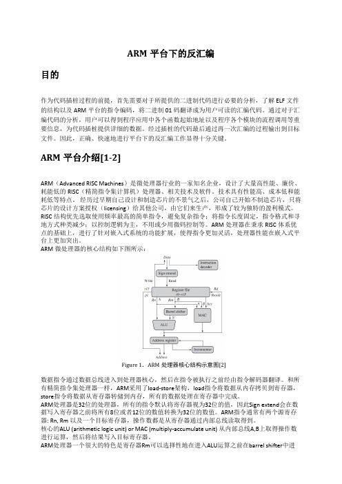
ARM微处理器的核心结构如下图所示：Figure 1．ARM处理器核心结构示意图[2]数据指令通过数据总线进入到处理器核心，然后在指令被执行之前经由指令解码器翻译。

和所有精简指令集处理器一样，ARM采用了load-store架构，load指令将数据从内存拷贝到寄存器，store指令将数据从寄存器转储到内存，所有的数据处理在寄存器中完成。

ARM处理器是32位的处理器，所有的指令默认将寄存器视为32位的值，因此Sign extend会在数据写入寄存器之前将所有8位或者12位的数值转换为32位的数值。

ARM指令通常有两个源寄存器: Rn, Rm 以及一个目标寄存器，操作数都是从寄存器通过内部总线读取得到。

专利名称：PRIORITY CONTROL SYSTEM FOR INTERPRETER发明人：YAMADA KENICHI申请号：JP1039088申请日：19880120公开号：JPH01185759A公开日：19890725专利内容由知识产权出版社提供摘要：PURPOSE:To attain the priority processing of a command by executing the processing of the priority command data in a priority interpreter immediately after priority command data inputted to a First-In First-Out (FIFO) buffer is detected. CONSTITUTION:A normal interpreter 2 sequentially processes command data CD in the FIFO buffer 3 in the order of the time of their generation. An input processing part 1A controls the input of command data at a prescribed period prior to the normal interpreter 2, while said part retrieves command data CD and immediately gives an execution right to the normal interpreter 2 when priority command data CDA is inputted to the FIFO buffer 3. The priority interpreter 2A extracts priority command data CDA, and gives the execution right to the normal interpreter 2 after the priority command data is processed. Thus, the priority processing of command data can be executed.申请人：FUJI ELECTRIC CO LTD,FUJI FACOM CORP更多信息请下载全文后查看。

IncrediBuild⼯具使⽤及设置（转）虽然现在计算机的运算速度不断提⾼, 但⼤型软件的编译速度仍然是个漫长的过程,我所在的项⽬, 软件⼤⼩约为200K⾏, 在VC6下的编译时间为3分钟(P4 1.8G, 512M), 在交叉编译时更慢, 提⾼编译速度将能够直接提⾼前期调测的效率. 本⽂将介绍提⾼编译速度的有效⽅法之⼀ - 分布式编译.分布式编译的原理很简单, 就是将编译的整个⼯作量通过分布计算的⽅法分配到多个计算机上执⾏, 这样可以获得极⼤的效率提升. 由于分布式计算的技术相对成熟, 现在可以见到的分布式编译软件也较多. ⼀般来说, ⼀个分布式编译软件不是⼀个编译器, ⽽是附着在某个编译器上的分布计算管理软件, 使得对于特定的编译器可以实现分布式编译.常见的分布式编译器通常是对应于特定的C/C++编译器, 如Gcc, Visual C++, 因为这些编译器使⽤相当⼴泛且开放度⾼. 因⽽实现分布式编译的意义更⼤. 下⾯分别以Visual C++和Gcc为例说明两个典型的分布式编译软件:1)IncrediBuild这是⼀个对应Visual C++ 的分布式编译软件, 通过Visual C++强⼤的IDE扩展功能, 它有着⾮常友好的界⾯, 可以将整个分布式编译过程直观的展现给⽤户, 并且它通过⼀个"虚拟机"的技术, 使能编译的参与者可以与编译发起者有着不同的系统配置(Windows操作系统版本, 库⽂件等),甚⾄⽆需在参与者机器上安装Visual C++.IncrediBuild需要⼀个特定的计算机做仲裁者, 其他的所有计算机作为客户, 有了仲裁者的好处是, 可以有它来统⼀安排所有客户端所发起的编译请求, ⼀旦某个客户发起编译请求, 则仲裁者会根据其他客户的CPU空闲情况⽽安排分布式编译, 当多个客户同时发起编译请求时, 仲裁者会⾃动平衡分布计算负担,使得编译参与者不会占⽤过多的CPU.在我们的项⽬中, 使⽤IncrediBuild的结果如下:未使⽤: 3分钟5客户: 40秒10客户: 25秒可见IncrediBuild对编译性能的巨⼤提升, 并且在取得如此性能提升的同时, 仲裁者和编译参与者的CPU占⽤率很低. 保持相当⾼的可⽤性, 这是很难得的.IncridiBuild的缺点是⽬前仅⽀持Visual C++ 6编译器和.Net编译器, 也仅适⽤于Windows平台. 适⽤范围相对较窄.2)DistCC这是⼀个GNU的分布式C++编译器, 适⽤于⼀切Gcc兼容的C++编译器, DistCC也具有很好的跨平台特性, ⽀持Linux, XFree86, CygWin等平台. 使⽤范围相当⼴泛.DistCC和IncrediBuild的差别在与DistCC不使⽤仲裁者, 直接由客户端对其他客户端发起编译请求. 所以每个客户端都需要知道其他客户端的位置, 并且当多个客户发起编译请求时不易做平衡处理.下⾯说⼀下怎样利⽤increbuild实现分布式编译1.make⽂件夹⾥⾯的Gsm2.mak修改make⼯具的编译项为IncredBuild增加运⾏参数#@echo tools/make.exe -fmake/comp.mak -r -R COMPONENT=$* ... $(strip $(COMPLOGDIR))/$*.log@if /I %OS% EQU WINDOWS_NT /(if /I $(BM_NEW) EQU TRUE /(XGConsole /command="tools/make.exe -fmake/comp.mak -k -r -R $(strip $(CMD_ARGU)) COMPONENT=$* > $(strip $(COMPLOGDIR))/$*.log 2>&1" /NOLOGO /profile="tools/XGConsole.xml") /else /(XGConsole /command="tools/make.exe -fmake/comp.mak -r -R $(strip $(CMD_ARGU)) COMPONENT=$* > $(strip $(COMPLOGDIR))/$*.log 2>&1" /NOLOGO /profile="tools/XGConsole.xml") /) /else /(if /I $(BM_NEW) EQU TRUE /(tools/make.exe -fmake/comp.mak -k -r -R $(strip $(CMD_ARGU)) COMPONENT=$* > $(strip $(COMPLOGDIR))/$*.log) /else /(tools/make.exe -fmake/comp.mak -r -R $(strip $(CMD_ARGU)) COMPONENT=$* > $(strip $(COMPLOGDIR))/$*.log) /)@type $(strip $(COMPLOGDIR))/$*.log >> $(LOG)@perl ./tools/chk_lib_err_warn.pl $(strip $(COMPLOGDIR))/$*.log2.tools⼯具夹⾥⾯加⼊ XGConsole.xml内容为<?xml version="1.0" encoding="UTF-8" standalone="no" ?><Profile FormatVersion="1"><Tools><Tool Filename="perl" AllowRemote="true" /><Tool Filename="make" AllowIntercept="true" /><Tool Filename="tcc" AllowRemote="true" /><Tool Filename="tcpp" AllowRemote="true" /><Tool Filename="armcc" AllowRemote="true" /><Tool Filename="armcpp" AllowRemote="true" /><Tool Filename="strcmpex" AllowRemote="true" /><Tool Filename="warp" AllowRemote="true" /></Tools></Profile>3.tools⼯具夹⾥⾯的make2.pl修改以下⼏⾏if (($action eq "update") || ($action eq "remake") || ($action eq "new") || ($action eq "bm_new") ||($action eq "c,r") || ($action eq "c,u")){if ($ENV{"NUMBER_OF_PROCESSORS"} > 1){if ($fullOpts eq ""){$fullOpts = "CMD_ARGU=-j$ENV{/"NUMBER_OF_PROCESSORS/"}";}else{$fullOpts .= ",-j$ENV{/"NUMBER_OF_PROCESSORS/"}";}}}改为if (($action eq "update") || ($action eq "remake") || ($action eq "new") || ($action eq "bm_new") ||($action eq "c,r") || ($action eq "c,u")){if ($ENV{"NUMBER_OF_PROCESSORS"} >= 1){if ($fullOpts eq ""){$fullOpts = "CMD_ARGU=-j$ENV{/"NUMBER_OF_PROCESSORS/"}"."0";}else{$fullOpts .= ",-j$ENV{/"NUMBER_OF_PROCESSORS/"}"."0";}}}$ENV{"NUMBER_OF_PROCESSORS"} = 10; //修改为你想要的进程数4.把tools⾥⾯的make.exe换成多任务的⽂件联合编译的功能引⼊分为下⾯⼏个要素：1．使能或禁⽌联合编译功能；2．检查XGC是否存在；3．定义可⽤的进程数；4．中间编译⽂件；5．编译命令；1.1. 使能或禁⽌联合编译的参数设定对于MTK平台，可以通过命令⾏⽅式参数“-disable_ib”，“-no_ib”或“-bm”。

Fortran 编译器---------------------------------------------------------------------------------------1. Fortran Powerstation 4.0Fortran Powerstation 4.0是最老的版本下载ftp://2006:2006@/36/-002123.ZIP---------------------------------------------------------------------------------------2.CVFCompaq Visual Fortran （CVF）, 当今PC平台上功能相当强大与完整的Fortran程序开发工具，还用于Abaqus的开发。

1997年，微软将Fortran PowerStation卖给DEC之后，微软就不再出版Fortran编译器了。

后来DEC并入了Compaq，再后来Compaq又和HP合并了。

现在最新的版本是HP出的Fortran for Windows v6.6，现在HP/Compaq已经不再开发Fortran了，CVF 6.6是最终的版本了，Compaq的Fortran开发小组已经投入Intel旗下，目前Intel 已经有Intel Visual Fortran 11.0。

Compaq Visual Fortran 6.6官方的单价也相当昂贵。

Compaq Visual Fortran 6.6 下载：/SoftDown.asp?ID=11937Compaq Visual Fortran 6.6 绿色版下载：/down/10915.htmlCompaq Visual Fortran 6.5 下载：/soft/fortran6.5.rarftp://2006:2006@/36/-002124.rar---------------------------------------------------------------------------------------3. IVFIntel Visual Fortran (IVF)将Compaq Visual Fortran* (CVF) 语言的丰富功能与英特尔代码生成及优化技术结合在一起。

【麦子学院】python命令执行3大方法总结在python开发中，我们常常需要执行命令，修改相关信息。

那对于初学者来说，python中如何执行命令呢？今天，小编就为大家分享3种python命令执行的方法。

1. 使用os.system("cmd")在python中，使用os.system("cmd")的最大特点是，其执行时程序会打出cmd在linux上执行的信息。

import osos.system("ls")2. 使用Popen模块产生新的processPopen是现在python开发者最喜欢使用的命令执行方法，虽然Popen不会像os.system方法一样，打出cmd在linux上执行的信息，但Popen支持多种参数和模式，使用前需要from subprocess import Popen, PIPE。

Popen方法很强大，这不容置疑，但其仍存在一个明显的缺陷，那就是他是一个阻塞方法。

如果运行cmd时产生的内容非常多，Popen函数就非常容易阻塞住。

解决办法是不使用wait()方法，但是也不能获得执行的返回值了。

Popen原型是：subprocess.Popen(args, bufsize=0, executable=None, stdin=None, stdout=None, stderr=None, preexec_fn=None, close_fds=False, shell=False, cwd=None, env=None, universal_newlines=False, startupinfo=None, creationflags=0)参数bufsize：指定缓冲。

参数executable用于指定可执行程序。

一般情况下我们通过args参数来设置所要运行的程序。

如果将参数shell设为 True，executable将指定程序使用的shell。

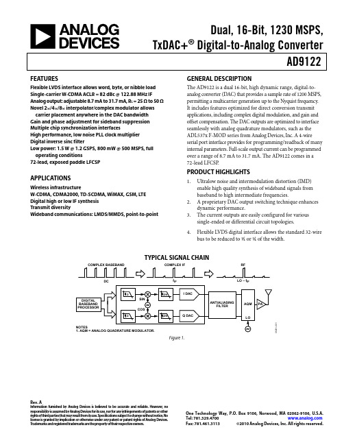
Dual, 16-Bit, 1230 MSPS,TxDAC+® Digital-to-Analog ConverterAD9122 Rev. AInformation furnished by Analresponsibility is assumed by Ana rights of third parties that may re license is granted by implication T rademarks and registered trad MA 02062-9106, U.S.A. Inc. All rights reserved.og Devices is believed to be accurate and reliable. However, nolog Devices for its use, nor for any infringements of patents or other sult from its use. Specifications subject to change without notice. No or otherwise under any patent or patent rights of Analog Devices. emarks are the property of their respective owners. One Technology Way, P.O. Box 9106, Norwood, Tel: 781.329.4700Fax: 781.461.3113 ©2010 Analog Devices,FEATURESFlexible LVDS interface allows word, byte, or nibble load Single-carrier W-CDMA ACLR = 82 dBc @ 122.88 MHz IF Analog output: adjustable 8.7 mA to 31.7 mA, R L = 25 Ω to 50 Ω Novel 2×/4×/8× interpolator/complex modulator allows carrier placement anywhere in the DAC bandwidthGain and phase adjustment for sideband suppression Multiple chip synchronization interfacesHigh performance, low noise PLL clock multiplierDigital inverse sinc filterLow power: 1.5 W @ 1.2 GSPS, 800 mW @ 500 MSPS, full operating conditions72-lead, exposed paddle LFCSPAPPLICATIONSWireless infrastructureW-CDMA, CDMA2000, TD-SCDMA, WiMAX, GSM, LTEDigital high or low IF synthesisTransmit diversityWideband communications: LMDS/MMDS, point-to-point GENERAL DESCRIPTIONThe AD9122 is a dual 16-bit, high dynamic range, digital-to-analog converter (DAC) that provides a sample rate of 1200 MSPS, permitting a multicarrier generation up to the Nyquist frequency. It includes features optimized for direct conversion transmit applications, including complex digital modulation, and gain and offset compensation. The DAC outputs are optimized to interface seamlessly with analog quadrature modulators, such as the ADL537x F-MOD series from Analog Devices, Inc. A 4-wire serial port interface provides for programming/readback of many internal parameters. Full-scale output current can be programmed over a range of 8.7 mA to 31.7 mA. The AD9122 comes in a 72-lead LFCSP.PRODUCT HIGHLIGHTS1.Ultralow noise and intermodulation distortion (IMD)enable high quality synthesis of wideband signals frombaseband to high intermediate frequencies.2. A proprietary DAC output switching technique enhancesdynamic performance.3.The current outputs are easily configured for varioussingle-ended or differential circuit topologies.4.Flexible LVDS digital interface allows the standard 32-wirebus to be reduced to ½ or ¼ of the width.TYPICAL SIGNAL CHAINCOMPLEX BASEBANDDC COMPLEX IFf IFRFLO – f IF8281-1 Figure 1.AD9122Rev. A | Page 2 of 60TABLE OF CONTENTSFeatures .............................................................................................. 1 Applications ....................................................................................... 1 General Description ......................................................................... 1 Product Highlights ........................................................................... 1 Typical Signal Chain ......................................................................... 1 Revision History ............................................................................... 3 Functional Block Diagram .............................................................. 4 Specifications ..................................................................................... 5 DC Specifications ......................................................................... 5 Digital Specifications ................................................................... 6 Digital Input Data Timing Specifications ................................. 6 AC Specifications .......................................................................... 7 Absolute Maximum Ratings ............................................................ 8 Thermal Resistance ...................................................................... 8 ESD Caution .................................................................................. 8 Pin Configuration and Function Descriptions ............................. 9 Typical Performance Characteristics ........................................... 11 Terminology .................................................................................... 17 Differences Between the AD9122R1 and AD9122R2 ............... 18 Theory of Operation ...................................................................... 19 Serial Port Operation ................................................................. 19 Data Format ................................................................................ 19 Serial Port Pin Descriptions ...................................................... 19 Serial Port Options ..................................................................... 20 Device Configuration Register Map and Descriptions ......... 21 LVDS Input Data Ports .................................................................. 33 Word Interface Mode ................................................................. 33 Byte Interface Mode ................................................................... 33 Nibble Interface Mode ............................................................... 33 FIFO Operation .......................................................................... 33 Interface Timing ......................................................................... 35 Digital Datapath .............................................................................. 37 Premodulation ............................................................................ 37 Interpolation Filters ................................................................... 37 NCO Modulation ....................................................................... 40 Datapath Configuration ............................................................ 40 Determining Interpolation Filter Modes ................................ 41 Datapath Configuration Example ............................................ 42 Data Rates vs. Interpolation Modes ......................................... 43 Coarse Modulation Mixing Sequences .................................... 43 Quadrature Phase Correction ................................................... 44 DC Offset Correction ................................................................ 44 Inverse Sinc Filter ....................................................................... 44 DAC Input Clock Configurations ................................................ 45 DAC Input Clock Configurations ............................................ 45 Analog Outputs............................................................................... 47 Transmit DAC Operation .......................................................... 47 Auxiliary DAC Operation ......................................................... 48 Baseband Filter Implementation .............................................. 49 Driving the ADL5375-15 .......................................................... 49 Reducing LO Leakage and Unwanted Sidebands .................. 50 Device Power Dissipation .............................................................. 51 Temperature Sensor ................................................................... 52 Multichip Synchronization ............................................................ 53 Synchronization with Clock Multiplication ............................... 53 Synchronization with Direct Clocking .................................... 54 Data Rate Mode Synchronization ............................................ 54 FIFO Rate Mode Synchronization ........................................... 55 Additional Synchronization Features ...................................... 55 Interrupt Request Operation ........................................................ 57 Interrupt Service Routine .......................................................... 57 Interface Timing Validation .......................................................... 58 SED Operation ............................................................................ 58 SED Example .............................................................................. 58 Example Start-Up Routine ........................................................ 59 Outline Dimensions ....................................................................... 60 Ordering Guide .. (60)AD9122Rev. A | Page 3 of 60REVISION HISTORY3/10—Rev. 0 to Rev. AChanges to Reflect Differences Between R1 and R2Silicon................................................................................... Universal Changes to Features Section ............................................................ 1 Changes to Table 1 ............................................................................ 5 Changes to Table 2 ............................................................................ 6 Changes to Table 5 ............................................................................ 7 Change to IOVDD Rating in Table 6 .............................................. 8 Changes to Table 8 ............................................................................ 9 Changes to Figure 10 to Figure 15 ................................................ 12 Added Differences Between the AD9122R1 and AD9122R2 Section, Added Figure 36 and Figure 37; RenumberedSequentially ...................................................................................... 18 Changes to Table 10 ........................................................................ 21 Changes to Table 11 ........................................................................ 23 Changes to FIFO Operation Section ............................................ 33 Changes to Resettling the FIFO Section and Replaced Table 13; Renumbered Sequentially; Added Serial Port Initiated FIFO Reset Section, and Added FRAME Initiated Relative FIFOReset Section .................................................................................... 34 Added FRAME Initiated Absolute FIFO Reset Section andReplaced Table 14 ............................................................................ 35 Changes to Figure 54 ...................................................................... 38 Changes to Table 18 ........................................................................ 39 Changes to SED Example Section ................................................. 58 Added Example Start-Up Routine Section .................................. 59 9/09—Revision 0: Initial VersionAD9122Rev. A | Page 4 of 60FUNCTIONAL BLOCK DIAGRAMD15P—D15ND0P—D0NIOUT1P IOUT1NIOUT2P IOUT2NFSADJREFIO DCI FRAME08281-002Figure 2. AD9122 Functional Block DiagramAD9122Rev. A | Page 5 of 60SPECIFICATIONSDC SPECIFICATIONST MIN to T MAX , AVDD33 = 3.3 V , DVDD18 = 1.8 V , CVDD18 =1.8 V , I OUTFS = 20 mA, maximum sample rate, unless otherwise noted. Table 1.Parameter Min Typ Max Unit RESOLUTION 16 Bits ACCURACY Differential Nonlinearity (DNL) ±2.1 LSB Integral Nonlinearity (INL) ±3.7 LSB MAIN DAC OUTPUTS Offset Error −0.001 0 +0.001 % FSR Gain Error (with Internal Reference) −3.6 ±2 +3.6 % FSR Full-Scale Output Current 18.66 19.6 31.66 mA Output Compliance Range −1.0 +1.0 V Output Resistance 10 MΩ Gain DAC Monotonicity Guaranteed Settling Time to Within ±0.5 LSB 20 ns MAIN DAC TEMPERATURE DRIFT Offset 0.04 ppm/°C Gain 100 ppm/°C Reference Voltage 30 ppm/°C REFERENCE Internal Reference Voltage 1.2 V Output Resistance 5 kΩ ANALOG SUPPLY VOLTAGES AVDD33 3.13 3.3 3.47 V CVDD18 1.71 1.8 1.89 V DIGITAL SUPPLY VOLTAGES DVDD18 1.71 1.8 1.89 V IOVDD 1.71 1.8/3.3 3.47 V POWER CONSUMPTION 2× Mode, f DAC = 491.22 MSPS, IF = 10 MHz, PLL Off 834 mW 2× Mode, f DAC = 491.22 MSPS, IF = 10 MHz, PLL On 913 mW 8× Mode, f DAC = 800 MSPS, IF = 10 MHz, PLL Off 1135 1241 mWAVDD33 55 57 mA CVDD18 85 90 mA DVDD18 444 495 mA Power-Down Mode (Register 0x01 = 0xF1) 6.5 18.8 mW Power Supply Rejection Ratio, AVDD33 −0.3 +0.3 % FSR/V OPERATING RANGE −40 +25 +85 °C1Based on a 10 kΩ external resistor.AD9122Rev. A | Page 6 of 60DIGITAL SPECIFICATIONST MIN to T MAX , AVDD33 = 1.8 V , IOVDD = 3.3 V , DVDD18 = 1.8 V , CVDD18 = 1.8 V , I OUTFS = 20 mA, maximum sample rate, unless otherwise noted.1LVDS receiver is compliant to the IEEE 1596 reduced range link, unless otherwise noted.DIGITAL INPUT DATA TIMING SPECIFICATIONSTable 3.Parameter Min Typ Max UnitLATENCY (DACCLK Cycles) 1× Interpolation (With or Without Modulation) 64 Cycles 2× Interpolation (With or Without Modulation) 135 Cycles 4× Interpolation (With or Without Modulation) 292 Cycles 8× Interpolation (With or Without Modulation) 608 Cycles Inverse Sinc 20 Cycles Fine Modulation 8 Cycles Power-Up Time 260 msAD9122Rev. A | Page 7 of 60AC SPECIFICATIONST MIN to T MAX , AVDD33 = 3.3 V , DVDD18 = 1.8 V , CVDD18 = 1.8 V , I OUTFS = 20 mA, maximum sample rate, unless otherwise noted. Table 4.ParameterMin Typ Max UnitSPURIOUS-FREE DYNAMIC RANGE (SFDR) f DAC = 100 MSPS, f OUT = 20 MHz 78 dBc f DAC = 200 MSPS, f OUT = 50 MHz 80 dBc f DAC = 400 MSPS, f OUT = 70 MHz 69 dBc f DAC = 800 MSPS, f OUT = 70 MHz72 dBc TWO-TONE INTERMODULATION DISTORTION (IMD) f DAC = 200 MSPS, f OUT = 50 MHz 84 dBc f DAC = 400 MSPS, f OUT = 60 MHz 86 dBc f DAC = 400 MSPS, f OUT = 80 MHz 84 dBc f DAC = 800 MSPS, f OUT = 100 MHz81 dBc NOISE SPECTRAL DENSITY (NSD) EIGHT-TONE, 500 kHz TONE SPACING f DAC = 200 MSPS, f OUT = 80 MHz −162 dBm/Hz f DAC = 400 MSPS, f OUT = 80 MHz −163 dBm/Hz f DAC = 800 MSPS, f OUT = 80 MHz−164 dBm/Hz W-CDMA ADJACENT CHANNEL LEAKAGE RATIO (ACLR), SINGLE CARRIER f DAC = 491.52 MSPS, f OUT = 10 MHz 84 dBc f DAC = 491.52 MSPS, f OUT = 122.88 MHz 82 dBc f DAC = 983.04 MSPS, f OUT = 122.88 MHz 83 dBc W-CDMA SECOND ACLR, SINGLE CARRIER f DAC = 491.52 MSPS, f OUT = 10 MHz 88 dBc f DAC = 491.52 MSPS, f OUT = 122.88 MHz 86 dBc f DAC = 983.04 MSPS, f OUT = 122.88 MHz88dBcTable 5. Interface SpeedsBus Width Interpolation Factorf BUS (Mbps)1.8 V ± 5% 1.8 V ± 2% 1.9 V ± 5% Nibble (4 Bits) 1×1100 1200 1230 2× (HB1) 1100 1200 1230 2× (HB2) 1100 1200 1230 4× 1100 1200 1230 8× 1100 1200 1230 Byte (8 Bits) 1×1100 1200 1230 2× (HB1) 1100 1200 1230 2× (HB2) 1100 1200 1230 4× 1100 1200 1230 8× 550 600 615 Word (16 Bits) 1×1100 1200 1230 2× (HB1) 900 1000 1000 2× (HB2) 1100 1200 1230 4× 550 600 615 8×275 300 307.5AD9122Rev. A | Page 8 of 60ABSOLUTE MAXIMUM RATINGSTHERMAL RESISTANCEThe exposed paddle (EPAD) must be soldered to the ground plane for the 72-lead, LFCSP . The EPAD performs as an electrical and thermal connection to the board.Typical θJA , θJB , and θJC are specified for a 4-layer board in still air. Airflow increases heat dissipation effectively reducing θJA and θJB . Table 7. Thermal ResistancePackage θJA θJB θJC Unit Conditions 72-Lead LFCSP_VQ 20.7 10.9 1.1 °C/W EPAD solderedESD CAUTIONStresses above those listed under Absolute Maximum Ratings may cause permanent damage to the device. This is a stress rating only; functional operation of the device at these or any other conditions above those indicated in the operationalsection of this specification is not implied. Exposure to absolute maximum rating conditions for extended periods may affect device reliability.AD9122Rev. A | Page 9 of 6008281-003D 11P D 11N D 10P D 10N D 9P D 9N D 8P D 8N D C I D C I D V D D 18D V S D 7P D 7N D 6P D 6N D 5P D 5N PIN CONFIGURATION AND FUNCTION DESCRIPTIONS12345678910111213141516CVDD18DACCLKP DACCLKNCVSS FRAMEP FRAMENIRQ D15P D15N NC IOVDD DVDD18D14P D14N D13P D13N 17D12P 18D12N 19202122232425262728293031323334P N S 3536545352515049484746454443424140393837RESET CS SCLK SDIO SDO DVDD18D0N D0P D1N D1P DVSS DVDD18D2N D2P D3N D3P D4N D4P727170696867666564636261605958575655C VD D 18C V D D 18REF C L K P R E F C L K N A V D D 33I O U T 1P I O U T 1N A V D D 33A V S S F S A D J R E F I O A V S S A V D D 33I O U T 2N I O U T 2P A V D D 33A V S S NCNOTES1. NC = NO CONNECT.2. EXPOSED PAD MUST BE CONNECTED TO AVSS.Figure 3. Pin ConfigurationAD9122Rev. A | Page 10 of 60AD9122050100150200250300350400450f OUT (MHz)TYPICAL PERFORMANCE CHARACTERISTICS0–10–20–30–40–50–60–70–80–90–100H A R M O N I C S (d B c)08281-10150100150200250300350400450f OUT (MHz)Figure 4. Harmonics vs. f OUT over f DATA , 2× Interpolation,Digital Scale = 0 dBFS, f SC = 20 mA0–10–20–30–40–50–60–70–80–90–100H A R M O N I C S (d B c )08281-10208281-1030–10–20–30–40–50–60–70–80–90–100050100150200250300350400450H A R M O N I C S (d B c )f OUT(MHz)08281-1040–10–20–30–40–50–60–70–80–90–10050100150200250300350400450H A R M O N I C S (d B c )f OUT (MHz)Figure 7. Second Harmonic vs. f OUT over Digital Scale, 2× Interpolation,f DATA = 400 MSPS, f SC= 20 mA08281-1050–10–20–30–40–50–60–70–80–90–10050100150200250300350400450H A R M O N I C S (d B c )f OUT (MHz)Figure 5. Harmonics vs. f OUT over f DATA , 4× Interpolation,Digital Scale = 0 dBFS, f SC = 20 mAFigure 8. Third Harmonic vs. f OUT over Digital Scale, 2× Interpolation,f DATA = 400 MSPS, f SC = 20 mA0–10–20–30–40–50–60–70–80–90–100H A R M O N I C S (d B c )100200300400500600700f OUT (MHz)08281-106Figure 6. Harmonics vs. f OUT over f DATA , 8× Interpolation,Digital Scale = 0 dBFS, f SC = 20 mA Figure 9. Second Harmonic vs. f OUT over f SC , 2× Interpolation,f DATA = 400 MSPS, Digital Scale = 0 dBFSAD9122–69–70–71–72–73–74–75–77H I G H E S T D I G I T A L S P U R (d B c )–78–79050100150200250300350400450f OUT (MHz)–7608281-10708281-110START 1.0MHz #RES BW 10kHzVBW 10kHzSTOP 500.0MHzSWEEP 6.017s (601 PTS)08281-111START 1.0MHz #RES BW 10kHzVBW 10kHzSTOP 800.0MHzSWEEP 9.634s (601 PTS)Figure 10. Highest Digital Spur vs. f OUT over f DATA , 2× Interpolation,Digital Scale = 0 dBFS, f SC = 20 mA–60–65–70–75–80–85H I G H E S T D I G I T A L S P U R (d B c )050100150200250300350400450f OUT (MHz)08281-108Figure 11. Highest Digital Spur vs. f OUT over f DATA , 4× Interpolation,Digital Scale = 0 dBFS, f SC = 20 mA–60–90–95–85–80–75–70–65H I G H E S T D I G I T A L S P U R (d B c )010*******400500600700f OUT (MHz)08281-109Figure 12. Highest Digital Spur vs. f OUT over f DATA , 8× Interpolation,Digital Scale = 0 dBFS, f SC = 20 mAFigure 13. 2× Interpolation, Single-Tone Spectrum, f DATA = 250 MSPS,f OUT= 101 MHzFigure 14. 4× Interpolation, Single-Tone Spectrum, f DATA = 200 MSPS,f OUT = 151 MHz08281-START 1.0MHz #RES BW 10kHzVBW 10kHzSTOP 800.0MHzSWEEP 9.634s (601 PTS)112Figure 15. 8× Interpolation, Single-Tone Spectrum, f DATA = 100 MSPS,f OUT = 131 MHzAD91220–90–80–70–60–50–40–30–20–10I M D (d B c )050100150200250300350400450f OUT (MHz)308281-11Figure 16. IMD vs. f OUT over f DATA , 2× Interpolation,Digital Scale = 0 dBFS, f SC = 20 mA0–80–70–60–50–40–30–20–10–90I M D (d B c )050100150200250300350400450f OUT (MHz)408281-11Figure 17. IMD vs. f OUT over f DATA , 4× Interpolation,Digital Scale = 0 dBFS, f SC = 20 mA0–80–70–60–50–40–30–20–10I M D (d B c )–100–90050100150200250300350400450f OUT(MHz)08281-115Figure 18. IMD vs. f OUT over f DATA , 8× Interpolation,Digital Scale = 0 dBFS, f SC = 20 mA0–90–80–70–60–50–40–30–20–10050100150200250300350400450I M D (d B c )f OUT(MHz)08281-116Figure 19. IMD vs. f OUT over Digital Scale, 2× Interpolation,f DATA = 400 MSPS, f SC = 20 mA–50–85–80–75–70–65–60–55050100150200250300350400450I M D (d B c )f OUT (MHz)08281-117Figure 20. IMD vs. f OUT over f SC , 2× Interpolation, f DATA = 400 MSPS,Digital Scale = 0 dBFS–40–90–85–80–75–70–65–60–55–50–45I M D (d B c)050100150200250300350400450f OUT (MHz)08281-118Figure 21. IMD vs. f OUT , PLL On vs. PLL Off, 4× Interpolation, f DATA = 200 MSPS,Digital Scale = 0 dBFS, f SC = 20 mAAD9122–152–156–154–158–160–162–164––166N S D (d B m /H z )50100150200250300350400450f OUT (MHz)908281-11Figure 22. 1-Tone NSD vs. f OUT over Interpolation Rate, Digital Scale = 0 dBFS,f SC = 20 mA, PLL Off–154–158–156–160–162–164–166–168N S D (d B m /H z )050100150200250300350400450f OUT (MHz)08281-12Figure 23. 1-Tone NSD vs. f OUT over Digital Scale, f DATA = 200 MSPS,4× Interpolation, f SC = 20 mA, PLL Off–158–159–160–161–162–163–164–165N S D (d B m /H z )–166050100150200250300350400450f OUT (MHz)08281-121Figure 24. 1-Tone NSD vs. f OUT over Interpolation Rate, Digital Scale = 0 dBFS,f SC = 20 mA, PLL On 161.0–165.5–165.0–164.5–164.0–163.5–163.0–162.5–162.0–161.5050100150200250300350400450N S D (d B m /H z )f OUT(MHz)08281-122Figure 25. 8-Tone NSD vs. f OUT over Interpolation Rate, Digital Scale = 0 dBFS,f SC = 20 mA, PLL Off–161.0–166.5–165.5–166.0–165.0–164.5–164.0–163.5–163.0–162.5–162.0–161.5050100150200250300350400450N S D (d B m /H z )fOUT (MHz)08281-123Figure 26. 8-Tone NSD vs. f OUT over Digital Scale, f DATA = 200 MSPS,4× Interpolation, f SC = 20 mA, PLL Off–160–161–162–163–164–165–166N S D (d B m /H z)050100150200250300350400450f OUT (MHz)08281-124Figure 27. 8-Tone NSD vs. f OUT over Interpolation Rate, Digital Scale = 0 dBFS,f SC = 20 mA, PLL OnAD9122–77–84–83–82–81–80–79–78A C L R (d B c )–050100150200250fOUT (MHz)50–55–60–65–70–75–80–85–900100200300400500A C L R (dB c )f OUT(MHz)08281-12508281-128Figure 28. 1-Carrier W-CDMA ACLR vs. f OUT over Digital Scale,Adjacent Channel, PLL Off–78–88–86–84–82–80–90A C L R (dB c )050100150200250fOUT (MHz)08281-126Figure 29. 1-Carrier W-CDMA ACLR vs. f OUT over f DAC ,Alternate Channel, PLL Off–70–90–85–80–75A C L R (dB c )–95050100150200250fOUT (MHz)08281-127Figure 30. 1-Carrier W-CDMA ACLR vs. f OUT over f DAC ,Second Alternate Channel, PLL Off Figure 31. 1-Carrier W-CDMA ACLR vs. f OUT , Adjacent Channel,PLL On vs. PLL Off–70–72–74–76–78–80–82–84–86–88–900100200300400500A C L R (dB c )f OUT(MHz)08281-129Figure 32. 1-Carrier W-CDMA ACLR vs. f OUT , Alternate Channel,PLL On vs. PLL Off–70–95–90–85–80–75A C L R (dB c)0100200300400500f OUT (MHz)08281-130Figure 33. 1-Carrier W-CDMA ACLR vs. f OUT , Second Alternate Channel,PLL On vs. PLL OffAD912208281-131START 133.06MHz #RES BW 30kHzVBW 30kHz STOP 166.94MHzSWEEP 143.6ms (601 PTS)START 125.88MHz #RES BW 30kHz VBW 30kHz STOP 174.42MHzSWEEP 206.9ms (601 PTS)TOTAL CARRIER POWER –11.19dBm/15.3600MHz RRC FILTER: OFF FILTER ALPHA 0.22REF CARRIER POWER –16.89dBm/3.84000MHzLOWER UPPER OFFSET FREQ INTEG BW dBc dBm dBc dBm 1–16.92dBm 5.000MHz 3.840MHz –65.88–82.76–67.52–84.40RMS RESULTS FREQ LOWER UPPER OFFSET REF BW dBc dBm dBc dBm CARRIER POWER 5.00MHz 3.840MHz –75.96–85.96–77.13–87.13–10.00dBm/10.00MHz 3.840MHz –85.33–95.33–85.24–95.253.840MHz15.00MHz2.888MHz–95.81–95.81–85.43–95.4308281-1322–16.89dBm 10.00MHz 3.840MHz –68.17–85.05–69.91–86.793–17.43dBm 15.00MHz 3.840MHz–70.42–87.31–71.40–88.284–17.64dBmFigure 35. 1-Carrier W-CDMA ACLR Performance, IF = ~150 MHzFigure 34. 4-Carrier W-CDMA ACLR Performance, IF = ~150 MHzAD9122 TERMINOLOGYIntegral Nonlinearity (INL)INL is defined as the maximum deviation of the actual analog output from the ideal output, determined by a straight line drawn from zero scale to full scale.Differential Nonlinearity (DNL)DNL is the measure of the variation in analog value, normalized to full scale, associated with a 1 LSB change in digital input code. Offset ErrorThe deviation of the output current from the ideal of zero is called offset error. For IOUT1P, 0 mA output is expected when the inputs are all 0s. For IOUT1N, 0 mA output is expected when all inputs are set to 1.Gain ErrorThe difference between the actual and ideal output span. The actual span is determined by the difference between the output when all inputs are set to 1 and the output when all inputs are set to 0.Output Compliance RangeThe range of allowable voltage at the output of a current output DAC. Operation beyond the maximum compliance limits can cause either output stage saturation or breakdown, resulting in nonlinear performance.Temperature DriftTemperature drift is specified as the maximum change from the ambient (25°C) value to the value at either T MIN or T MAX. For offset and gain drift, the drift is reported in ppm of full-scale range (FSR) per degree Celsius. For reference drift, the drift is reported in ppm per degree Celsius.Power Supply Rejection (PSR)The maximum change in the full-scale output as the supplies are varied from minimum to maximum specified voltages. Settling TimeThe time required for the output to reach and remain within a specified error band around its final value, measured fromthe start of the output transition.Spurious Free Dynamic Range (SFDR)The difference, in decibels, between the peak amplitude of the output signal and the peak spurious signal within the dc to the Nyquist frequency of the DAC. Typically, energy in this band is rejected by the interpolation filters. This specification, therefore, defines how well the interpolation filters work and the effect of other parasitic coupling paths to the DAC output.Signal-to-Noise Ratio (SNR)SNR is the ratio of the rms value of the measured output signal to the rms sum of all other spectral components below the Nyquist frequency, excluding the first six harmonics and dc. The value for SNR is expressed in decibels.Interpolation FilterIf the digital inputs to the DAC are sampled at a multiple rate of f DATA (interpolation rate), a digital filter can be constructed that has a sharp transition band near f DATA/2. Images that typically appear around f DAC (output data rate) can be greatly suppressed. Adjacent Channel Leakage Ratio (ACLR)The ratio in decibels relative to the carrier (dBc) between the measured power within a channel relative to its adjacent channel. Complex Image RejectionIn a traditional two-part upconversion, two images are created around the second IF frequency. These images have the effect of wasting transmitter power and system bandwidth. By placing the real part of a second complex modulator in series with the first complex modulator, either the upper or lower frequency image near the second IF can be rejected.。

在E语言中，可以使用系统调用函数来执行外部程序。

其中，createprocess函数是用于创建并启动新进程的函数之一。

下面是一个简单的示例，演示如何使用E语言调用createprocess 函数来执行外部程序：```c#include <stdio.h>#include <windows.h>int main() {STARTUPINFO startupInfo = { 0 };PROCESS_INFORMATION processInfo = { 0 };const char* programPath = "notepad.exe"; // 外部程序的路径const char* commandLine = programPath; // 传递给外部程序的命令行参数// 初始化startupInfo结构体startupInfo.cb = sizeof(startupInfo);startupInfo.lpReserved = NULL;startupInfo.lpDesktop = NULL;startupInfo.lpTitle = NULL;startupInfo.dwFlags = STARTF_USESTDHANDLES;// 创建并启动新进程if (!CreateProcess(NULL, // 指向应用程序名称的指针commandLine, // 指向命令行的指针NULL, // 安全属性，通常为NULLNULL, // 指向线程环境的指针，通常为NULLFALSE, // 不继承句柄标志0, // 进程映像标志，通常为0NULL, // 指向环境变量的指针，通常为NULLNULL, // 指向当前目录的指针&startupInfo, // STARTUPINFO结构体指针，用于获取进程句柄等信息&processInfo)) // 进程信息结构体指针{printf("CreateProcess failed with error: %d\n", GetLastError());return 1;}// 等待进程结束并获取退出代码WaitForSingleObject(processInfo.hProcess, INFINITE);GetExitCodeProcess(processInfo.hProcess, &exitCode);CloseHandle(processInfo.hProcess);CloseHandle(processInfo.hThread);printf("Program exited with code: %d\n", exitCode);return 0;}```上述代码使用CreateProcess函数创建了一个新进程，执行了notepad.exe程序，并等待进程结束并获取退出代码。

set-executionpolicy unrestricted 命令-概述说明以及解释1. 引言1.1 概述在计算机技术的发展中，安全性一直是一个非常重要的问题。

随着各种网络攻击和恶意软件的出现，保护计算机系统免受潜在的威胁变得越来越重要。

而在Windows操作系统中，PowerShell是一种强大的工具，它可以利用脚本语言来自动化执行各种系统管理任务。

然而，默认情况下，Windows PowerShell限制了可以运行的脚本的权限。

这是因为脚本的执行可能会带来潜在的安全风险，特别是当脚本来自未知来源时。

为了保护计算机系统的安全，Windows PowerShell默认将脚本的执行策略设置为限制模式。

然而，有时候我们需要在特定的情况下解除这个限制，以便能够运行脚本。

在这种情况下，可以使用"set-executionpolicy unrestricted"命令来修改PowerShell的执行策略，使得可以执行任何脚本，无论其来源是否可信。

本文将介绍set-executionpolicy unrestricted命令的概念、意义以及在实际应用中的一些注意事项。

首先，我们将提供一些背景知识，介绍PowerShell和脚本执行策略的基本概念。

接着，我们将详细探讨set-executionpolicy unrestricted命令的作用和意义，并说明在什么情况下使用它是有必要的。

最后，我们将总结这个命令的优缺点，并提供一些建议，来帮助读者在使用set-executionpolicy unrestricted命令时注意安全性和潜在的风险。

通过深入了解set-executionpolicy unrestricted命令，读者将能够更好地理解PowerShell脚本的执行策略，并在必要时灵活运用这个命令来满足自己的需求。

而在使用这个命令时，我们也要始终牢记系统安全的重要性，并采取适当的措施来确保脚本的来源可信和执行的安全性。

Code maturity level options代码成熟度选项Prompt for development and/or incomplete code/drivers显示尚在开发中或尚未完成的代码与驱动.除非你是测试人员或者开发者,否则请勿选择General setup常规设置Local version - append to kernel release在内核版本后面加上自定义的版本字符串(小于64字符),可以用"uname -a"命令看到Automatically append version information to the version string 自动在版本字符串后面添加版本信息,编译时需要有perl以及git仓库支持Support for paging of anonymous memory (swap)使用交换分区或者交换文件来做为虚拟内存System V IPCSystem V进程间通信(IPC)支持,许多程序需要这个功能.必选,除非你知道自己在做什么IPC NamespacesIPC命名空间支持,不确定可以不选POSIX Message QueuesPOSIX消息队列,这是POSIX IPC中的一部分BSD Process Accounting将进程的统计信息写入文件的用户级系统调用,主要包括进程的创建时间/创建者/内存占用等信息BSD Process Accounting version 3 file format使用新的第三版文件格式,可以包含每个进程的PID和其父进程的PID,但是不兼容老版本的文件格式Export task/process statistics through netlink通过netlink接口向用户空间导出任务/进程的统计信息,与BSD Process Accounting的不同之处在于这些统计信息在整个任务/进程生存期都是可用的Enable per-task delay accounting在统计信息中包含进程等候系统资源(cpu,IO同步,内存交换等)所花费的时间UTS NamespacesUTS名字空间支持,不确定可以不选Auditing support审计支持,某些内核模块(例如SELinux)需要它,只有同时选择其子项才能对系统调用进行审计Enable system-call auditing support支持对系统调用的审计Kernel .config support把内核的配置信息编译进内核中,以后可以通过scripts/extract-ikconfig脚本来提取这些信息Enable access to .config through /proc/config.gz允许通过/proc/config.gz访问内核的配置信息Cpuset support只有含有大量CPU(大于16个)的SMP系统或NUMA(非一致内存访问)系统才需要它Kernel->user space relay support (formerly relayfs)在某些文件系统上(比如debugfs)提供从内核空间向用户空间传递大量数据的接口Initramfs source file(s)initrd已经被initramfs取代,如果你不明白这是什么意思,请保持空白Optimize for size (Look out for broken compilers!)编译时优化内核尺寸(使用"-Os"而不是"-O2"参数编译),有时会产生错误的二进制代码Enable extended accounting over taskstats收集额外的进程统计信息并通过taskstats接口发送到用户空间Configure standard kernel features (for small systems)配置标准的内核特性(为小型系统)Enable 16-bit UID system calls允许对UID系统调用进行过时的16-bit包装Sysctl syscall support不需要重启就能修改内核的某些参数和变量,如果你也选择了支持/proc,将能从/proc/sys存取可以影响内核行为的参数或变量Load all symbols for debugging/kksymoops装载所有的调试符号表信息,仅供调试时选择Include all symbols in kallsyms在kallsyms中包含内核知道的所有符号,内核将会增大300KDo an extra kallsyms pass除非你在kallsyms中发现了bug并需要报告这个bug才打开该选项Support for hot-pluggable devices支持热插拔设备,如usb与pc卡等,Udev也需要它Enable support for printk允许内核向终端打印字符信息,在需要诊断内核为什么不能运行时选择BUG() support显示故障和失败条件(BUG和WARN),禁用它将可能导致隐含的错误被忽略Enable ELF core dumps内存转储支持,可以帮助调试ELF格式的程序Enable full-sized data structures for core在内核中使用全尺寸的数据结构.禁用它将使得某些内核的数据结构减小以节约内存,但是将会降低性能Enable futex support快速用户空间互斥体可以使线程串行化以避免竞态条件,也提高了响应速度.禁用它将导致内核不能正确的运行基于glibc的程序Enable eventpoll support支持事件轮循的系统调用Use full shmem filesystem完全使用shmem来代替ramfs.shmem是基于共享内存的文件系统(可能用到swap),在启用TMPFS后可以挂载为tmpfs供用户空间使用,它比简单的ramfs先进许多Use full SLAB allocator使用SLAB完全取代SLOB进行内存分配,SLAB是一种优秀的内存分配管理器,推荐使用Enable VM event counters for /proc/vmstat允许在/proc/vmstat中包含虚拟内存事件记数器Loadable module support可加载模块支持Enable loadable module support打开可加载模块支持,如果打开它则必须通过"make modules_install"把内核模块安装在/lib/modules/中Module unloading允许卸载已经加载的模块Forced module unloading允许强制卸载正在使用中的模块(比较危险)Module versioning support允许使用其他内核版本的模块(可能会出问题)Source checksum for all modules为所有的模块校验源码,如果你不是自己编写内核模块就不需要它Automatic kernel module loading让内核通过运行modprobe来自动加载所需要的模块,比如可以自动解决模块的依赖关系Block layer块设备层Enable the block layer块设备支持,使用硬盘/USB/SCSI设备者必选Support for Large Block Devices仅在使用大于2TB的块设备时需要Support for tracing block io actions块队列IO跟踪支持,它允许用户查看在一个块设备队列上发生的所有事件,可以通过blktrace程序获得磁盘当前的详细统计数据Support for Large Single Files仅在可能使用大于2TB的文件时需要IO SchedulersIO调度器Anticipatory I/O scheduler假设一个块设备只有一个物理查找磁头(例如一个单独的SATA硬盘),将多个随机的小写入流合并成一个大写入流,用写入延时换取最大的写入吞吐量.适用于大多数环境,特别是写入较多的环境(比如文件服务器) Deadline I/O scheduler使用轮询的调度器,简洁小巧,提供了最小的读取延迟和尚佳的吞吐量,特别适合于读取较多的环境(比如数据库)CFQ I/O scheduler使用QoS策略为所有任务分配等量的带宽,避免进程被饿死并实现了较低的延迟,可以认为是上述两种调度器的折中.适用于有大量进程的多用户系统Default I/O scheduler默认IO调度器Processor type and features中央处理器(CPU)类型及特性Symmetric multi-processing support对称多处理器支持,如果你有多个CPU或者使用的是多核CPU就选上.此时"Enhanced Real Time Clock Support"选项必须开启,"Advanced Power Management"选项必须关闭Subarchitecture Type处理器的子架构,大多数人都应当选择"PC-compatible"Processor family处理器系列,请按照你实际使用的CPU选择Generic x86 support通用x86支持,如果你的CPU能够在上述"Processor family"中找到就别选HPET Timer SupportHPET是替代8254芯片的新一代定时器,i686及以上级别的主板都支持,可以安全的选上Maximum number of CPUs支持的最大CPU数,每增加一个内核将增加8K体积SMT (Hyperthreading) scheduler support支持Intel的超线程(HT)技术Multi-core scheduler support针对多核CPU进行调度策略优化Preemption Model内核抢占模式No Forced Preemption (Server)适合服务器环境的禁止内核抢占Voluntary Kernel Preemption (Desktop)适合普通桌面环境的自愿内核抢占Preemptible Kernel (Low-Latency Desktop)适合运行实时程序的主动内核抢占Preempt The Big Kernel Lock可以抢占大内核锁,应用于实时要求高的场合,不适合服务器环境Machine Check Exception让CPU检测到系统故障时通知内核,以便内核采取相应的措施(如过热关机等)Check for non-fatal errors on AMD Athlon/Duron / Intel Pentium 4 每5秒检测一次这些cpu的非致命错误并纠正它们,同时记入日志check for P4 thermal throttling interrupt当P4的cpu过热时显示一条警告消息Enable VM86 support虚拟X86支持,在DOSEMU下运行16-bit程序或XFree86通过BIOS初始化某些显卡的时候才需要Toshiba Laptop supportToshiba笔记本模块支持Dell laptop supportDell笔记本模块支持Enable X86 board specific fixups for reboot修正某些旧x86主板的重起bug,这种主板基本绝种了/dev/cpu/microcode - Intel IA32 CPU microcode support使用不随Linux内核发行的IA32微代码,你必需有IA32微代码二进制文件,仅对Intel的CPU有效/dev/cpu/*/msr - Model-specific register support在多cpu系统中让特权CPU访问x86的MSR寄存器/dev/cpu/*/cpuid - CPU information support能从/dev/cpu/x/cpuid获得CPU的唯一标识符(CPUID)Firmware Drivers固件驱动程序BIOS Enhanced Disk Drive calls determine boot disk有些BIOS支持从某块特定的硬盘启动(如果BIOS不支持则可能无法启动),目前大多数BIOS还不支持BIOS update support for DELL systems via sysfs仅适用于DELL机器Dell Systems Management Base Driver仅适用于DELL机器High Memory Support最高内存支持,总内存小于等于1G的选"off",大于4G的选"64G" Memory split如果你不是绝对清楚自己在做什么,不要改动这个选项Memory model一般选"Flat Memory",其他选项涉及内存热插拔64 bit Memory and IO resources使用64位的内存和IO资源Allocate 3rd-level pagetables from highmem在内存很多(大于4G)的机器上将用户空间的页表放到高位内存区,以节约宝贵的低端内存Math emulation数学协处理器仿真,486DX以上的cpu就不要选它了MTRR (Memory Type Range Register) support打开它可以提升PCI/AGP总线上的显卡2倍以上的速度,并且可以修正某些BIOS错误Boot from EFI supportEFI是一种可代替传统BIOS的技术(目前的Grub/LILO尚不能识别它),但是现在远未普及Enable kernel irq balancing让内核将irq中断平均分配给多个CPU以进行负载均衡,但是要配合irqbanlance守护进程才行Use register arguments使用"-mregparm=3"参数编译内核,将前3个参数以寄存器方式进行参数调用,可以生成更紧凑和高效的代码Enable seccomp to safely compute untrusted bytecode只有嵌入式系统可以不选Timer frequency内核时钟频率,桌面推荐"1000 HZ",服务器推荐"100 HZ"或"250 HZ" kexec system call提供kexec系统调用,可以不必重启而切换到另一个内核kernel crash dumps被kexec启动后产生内核崩溃转储Physical address where the kernel is loaded内核加载的物理地址,除非你知道自己在做什么,否则不要修改.在提供kexec系统调用的情况下可能要修改它Support for hot-pluggable CPUs对热插拔CPU提供支持Compat VDSO support如果Glibc版本大于等于2.3.3就不选,否则就选上Power management options电源管理选项Power Management support电源管理有APM和ACPI两种标准且不能同时使用.即使关闭该选项,X86上运行的Linux也会在空闲时发出HLT指令将CPU进入睡眠状态Legacy Power Management API传统的电源管理API,比如软关机和系统休眠等接口Power Management Debug Support仅供调试使用Driver model /sys/devices/.../power/state files内核帮助文档反对使用该选项,即将被废除ACPI (Advanced Configuration and Power Interface) Support 必须运行acpid守护程序ACPI才能起作用.ACPI是为了取代APM而设计的,因此应该尽量使用ACPI而不是APMAC Adapter如果你的系统可以在AC和电池之间转换就可以选Battery通过/proc/acpi/battery向用户提供电池状态信息,用电池的笔记本可以选Button守护程序捕获Power,Sleep,Lid按钮事件,并根据/proc/acpi/event做相应的动作,软件控制的poweroff需要它Video仅对集成在主板上的显卡提供ACPI2.0支持,且不是所有集成显卡都支持Generic Hotkey统一的热键驱动,建议不选Fan允许通过用户层的程序来对系统风扇进行控制(开,关,查询状态),支持它的硬件并不多Dock支持由ACPI控制的集线器(docking stations)Processor让ACPI处理空闲状态,并使用ACPI C2和C3处理器状态在空闲时节省电能,同时它还被cpufreq的"Performance-state drivers"选项所依赖Thermal Zone系统温度过高时可以利用ACPI thermal zone及时调整工作状态以避免你的CPU被烧毁ASUS/Medion Laptop ExtrasASUS笔记本专用,以提供额外按钮的支持,用户可以通过/proc/acpi/asus来打开或者关闭LCD的背光/调整亮度/定制LED的闪烁指示等功能IBM ThinkPad Laptop ExtrasIBM ThinkPad专用Toshiba Laptop ExtrasToshiba笔记本专用Disable ACPI for systems before Jan 1st this year输入四位数的年份,在该年的1月1日前不使用ACPI的功能("0"表示一直使用)Debug Statements详细的ACPI调试信息,不搞开发就别选Power Management Timer Support这个Timer在所有ACPI兼容的平台上都可用,且不会受PM功能的影响,建议总是启用它.如果你在kernel log中看到了'many lost ticks'那就必须启用它ACPI0004,PNP0A05 and PNP0A06 Container Driver支持内存和CPU的热插拔Smart Battery System支持依赖于I2C的"智能电池".这种电池非常老旧且罕见,还与当前的ACPI标准兼容性差APM (Advanced Power Management) BIOS SupportAPM在SMP机器上必须关闭,一般来说当前的笔记本都支持ACPI,所以应尽量关闭该该选项Ignore USER SUSPEND只有NEC Versa M系列的笔记本才需要选择这一项Enable PM at boot time系统启动时即启用APM,选上这个选项能让系统自动的进行电源管理,但常常导致启动时死机Make CPU Idle calls when idle系统空闲时调用空闲指令(halt),只有老式的CPU才需要选它,且对于SMP 系统必须关闭Enable console blanking using APM在屏幕空白时关闭LCD背光,事实上对所有的笔记本都无效RTC stores time in GMT将硬件时钟应该设为格林威治时间,否则视为本地时间.建议你使用GMT,这样你无须为时区的改变而担心Allow interrupts during APM BIOS calls允许APM的BIOS调用时中断,IBM Thinkpad的一些新机器需要这项.如果休眠时挂机(包括睡下去就醒不来),可以试试它Use real mode APM BIOS call to power off此驱动为某些有Bug的BIOS准备,如果你的系统不能正常关机或关机时崩溃,可以试试它CPU Frequency scaling允许动态改变CPU主频,达到省电和降温的目的,必须同时启用下面的一种governor才行Enable CPUfreq debugging允许对CPUfreq进行调试CPU frequency translation statistics通过sysfs文件系统输出CPU频率变换的统计信息CPU frequency translation statistics details输出详细的CPU频率变换统计信息Default CPUFreq governor默认的CPU频率调节器'performance' governor'性能'优先,静态的将频率设置为cpu支持的最高频率'powersave' governor'节能'优先,静态的将频率设置为cpu支持的最低频率'userspace' governor for userspace frequency scaling既允许手动调整cpu频率,也允许用户空间的程序动态的调整cpu频率(需要额外的调频软件,比如cpufreqd)'ondemand' cpufreq policy governor'立即响应',周期性的考察CPU负载并自动的动态调整cpu频率(不需要额外的调频软件),适合台式机'conservative' cpufreq governor'保守',和'ondemand'相似,但是频率的升降是渐变式的(幅度不会很大),更适合用于笔记本/PDA/AMD64环境ACPI Processor P-States driver将ACPI2.0的处理器性能状态报告给CPUFreq processor drivers以决定如何调整频率,该选项依赖于ACPI->Processor{省略的部分请按照自己实际使用的CPU选择}/proc/acpi/processor/../performance interface内核帮助文档反对使用该选项,即将被废除Relaxed speedstep capability checks放松对系统的speedstep兼容性检查,仅在某些老旧的Intel系统上需要打开Bus options (PCI, PCMCIA, EISA, MCA, ISA)总线选项PCI supportPCI支持,如果使用了PCI或PCI Express设备就必选PCI access modePCI访问模式,强列建议选"Any"(系统将优先使用"MMConfig",然后使用"BIOS",最后使用"Direct"检测PCI设备)PCI Express supportPCI Express支持(目前主要用于显卡和千兆网卡)PCI Express Hotplug driver如果你的主板和设备都支持PCI Express热插拔就可以选上Use polling mechanism for hot-plug events对热插拔事件采用轮询机制,仅用于测试目的Root Port Advanced Error Reporting support由PCI Express AER驱动程序处理发送到Root Port的错误信息Message Signaled Interrupts (MSI and MSI-X)PCI Express支持两类中断:INTx使用传统的IRQ中断,可以与现行的PCI 总线的驱动程序和操作系统兼容;MSI则是通过inbound Memory Write触发和发送中断,更适合多CPU系统.可以使用"pci=nomsi"内核引导参数关闭MSIPCI Debugging将PCI调试信息输出到系统日志里Interrupts on hypertransport devices允许本地的hypertransport设备使用中断ISA support现在基本上没有ISA的设备了,如果你有就选吧MCA support微通道总线,老旧的IBM的台式机和笔记本上可能会有这种总线NatSemi SCx200 support在使用AMD Geode处理器的机器上才可能有PCCARD (PCMCIA/CardBus) supportPCMCIA卡(主要用于笔记本)支持Enable PCCARD debugging仅供调试16-bit PCMCIA support一些老的PCMCIA卡使用16位的CardBus32-bit CardBus support当前的PCMCIA卡基本上都是32位的CardBusCardBus yenta-compatible bridge support使用PCMCIA卡的基本上都需要选择这一项,子项请按照自己实际使用的PCMCIA卡选择{省略的部分请按照自己实际使用的PCMCIA卡选择}PCI Hotplug SupportPCI热插拔支持,如果你有这样的设备就到子项中去选吧Executable file formats可执行文件格式Kernel support for ELF binariesELF是开放平台下最常用的二进制文件格式,支持动态连接,支持不同的硬件平台.除非你知道自己在做什么,否则必选Kernel support for a.out and ECOFF binaries早期UNIX系统的可执行文件格式,目前已经被ELF格式取代Kernel support for MISC binaries允许插入二进制的封装层到内核中,使用Java,.NET,Python,Lisp等语言编写的程序时需要它Networking网络Networking options网络选项Network packet debugging在调试不合格的包时加上额外的附加信息,但在遇到Dos攻击时你可能会被日志淹没Packet socket这种Socket可以让应用程序(比如tcpdump,iptables)直接与网络设备通讯,而不通过内核中的其它中介协议Packet socket: mmapped IO让Packet socket驱动程序使用IO映射机制以使连接速度更快Unix domain sockets一种仅运行于本机上的效率高于TCP/IP的Socket,简称Unix socket.许多程序都使用它在操作系统内部进行进程间通信(IPC),比如X Window和syslogTransformation user configuration interface为IPsec(可在ip层加密)之类的工具提供XFRM用户配置接口支持Transformation sub policy supportXFRM子策略支持,仅供开发者使用PF_KEY sockets用于可信任的密钥管理程序和操作系统内核内部的密钥管理进行通信,IPsec依赖于它TCP/IP networkingTCP/IP协议当然要选IP: multicasting群组广播,似乎与网格计算有关,仅在使用MBONE的时候才需要IP: advanced router高级路由,如果想做一个路由器就选吧IP: policy routing策略路由IP: equal cost multipath用于路由的基于目的地址的负载均衡IP: verbose route monitoring显示冗余的路由监控信息IP: kernel level autoconfiguration在内核启动时自动配置ip地址/路由表等,需要从网络启动的无盘工作站才需要这个东西IP: tunnelingIP隧道,将一个IP报文封装在另一个IP报文内的技术IP: GRE tunnels over IP基于IP的GRE(通用路由封装)隧道IP: multicast routing多重传播路由IP: ARP daemon support这东西尚处于试验阶段就已经被废弃了IP: TCP syncookie support抵抗SYN flood攻击的好东西,要启用它必须同时启用/proc文件系统和"Sysctl support",然后在系统启动并挂载了/proc之后执行"echo1 >/proc/sys/net/ipv4/tcp_syncookies"命令IP: AH transformationIPsec验证头(AH)实现了数据发送方的验证处理,可确保数据既对于未经验证的站点不可用也不能在路由过程中更改IP: ESP transformationIPsec封闭安全负载(ESP)实现了发送方的验证处理和数据加密处理,用以确保数据不会被拦截/查看或复制IP: IPComp transformationIPComp(IP静荷载压缩协议),用于支持IPsecIP: IPsec transport modeIPsec传输模式,常用于对等通信,用以提供内网安全.数据包经过了加密但IP头没有加密,因此任何标准设备或软件都可查看和使用IP头IP: IPsec tunnel modeIPsec隧道模式,用于提供外网安全(包括虚拟专用网络).整个数据包(数据头和负载)都已经过加密处理且分配有新的ESP头/IP头和验证尾,从而能够隐藏受保护站点的拓扑结构IP: IPsec BEET modeIPsec BEET模式INET: socket monitoring interfacesocket监视接口,一些Linux本地工具(如:包含ss的iproute2)需要使用它TCP: advanced congestion control高级拥塞控制,如果没有特殊需求(比如无线网络)就别选了,内核会自动将默认的拥塞控制设为"Cubic"并将"Reno"作为候补IP: Virtual Server ConfigurationIP虚拟服务器允许你基于多台物理机器构建一台高性能的虚拟服务器,不玩集群就别选了The IPv6 protocol你要是需要IPv6就选吧NetLabel subsystem supportNetLabel子系统为诸如CIPSO与RIPSO之类能够在分组信息上添加标签的协议提供支持,如果你看不懂就别选了Security Marking对网络包进行安全标记,类似于nfmark,但主要是为安全目的而设计,如果你不明白的话就别选Network packet filtering (replaces ipchains)Netfilter可以对数据包进行过滤和修改,可以作为防火墙("packet filter"或"proxy-based")或网关(NAT)或代理(proxy)或网桥使用.选中此选项后必须将"Fast switching"关闭,否则将前功尽弃Network packet filtering debugging仅供开发者调试Netfilter使用Bridged IP/ARP packets filtering如果你希望使用一个针对桥接的防火墙就打开它Core Netfilter Configuration核心Netfilter配置(当包流过Chain时如果match某个规则那么将由该规则的target来处理,否则将由同一个Chain中的下一个规则进行匹配,若不match所有规则那么最终将由该Chain的policy进行处理) Netfilter netlink interface允许Netfilter在与用户空间通信时使用新的netlink接口.netlink Socket是Linux用户态与内核态交流的主要方法之一,且越来越被重视.Netfilter NFQUEUE over NFNETLINK interface通过NFNETLINK接口对包进行排队Netfilter LOG over NFNETLINK interface通过NFNETLINK接口对包记录.该选项废弃了ipt_ULOG和ebg_ulog机制,并打算在将来废弃基于syslog的ipt_LOG和ip6t_LOG模块Layer 3 Independent Connection tracking独立于第三层的链接跟踪,通过广义化的ip_conntrack支持其它非IP协议的第三层协议Netfilter Xtables support如果你打算使用ip_tables,ip6_tables,arp_tables之一就必须选上"CLASSIFY" target support允许为包设置优先级,一些排队规则(atm,cbq,dsmark,pfifo_fast,htb,prio)需要使用它"CONNMARK" target support类似于"MARK",但影响的是连接标记的值"DSCP" target support允许对ip包头部的DSCP(Differentiated Services Codepoint)字段进行修改,该字段常用于Qos"MARK" target support允许对包进行标记(通常配合ip命令使用),这样就可以改变路由策略或者被其它子系统用来改变其行为"NFQUEUE" target Support用于替代老旧的QUEUE(iptables内建的target之一),因为NFQUEUE能支持最多65535个队列,而QUEUE只能支持一个"NOTRACK" target support允许规则指定哪些包不进入链接跟踪/NAT子系统"SECMARK" target support允许对包进行安全标记,用于安全子系统"CONNSECMARK" target support针对链接进行安全标记,同时还会将连接上的标记还原到包上(如果链接中的包尚未进行安全标记),通常与SECMARK target联合使用"comment" match support允许你在iptables规则集中加入注释"connbytes" per-connection counter match support允许针对单个连接内部每个方向(进/出)匹配已经传送的字节数/包数"connmark" connection mark match support允许针对每个会话匹配先前由"CONNMARK"设置的标记值"conntrack" connection tracking match support连接跟踪匹配,是"state"的超集,它允许额外的链接跟踪信息,在需要设置一些复杂的规则(比如网关)时很有用"DCCP" protocol match supportDCCP是打算取代UDP的新传输协议,它在UDP的基础上增加了流控和拥塞控制机制,面向实时业务"DSCP" match support允许对IP包头的DSCP字段进行匹配"ESP" match support允许对IPSec包中的ESP头进行匹配,使用IPsec的话就选上吧"helper" match support加载特定协议的连接跟踪辅助模块,由该模块过滤所跟踪的连接类型的包,比如ip_conntrack_ftp模块"length" match support允许对包的长度进行匹配"limit" match support允许根据包的进出速率进行规则匹配,常和"LOG target"配合使用以抵抗某些Dos攻击"mac" address match support允许根据以太网的MAC进行匹配,常用于无线网络环境"mark" match support允许对先前由"MARK"标记的特定标记值进行匹配IPsec "policy" match support使用IPsec就选上吧Multiple port match support允许对TCP或UDP包同时匹配多个端口(通常情况下只能匹配一个端口) "physdev" match support允许对到达的或将要离开的物理桥端口进行匹配"pkttype" packet type match support允许对封包目的地址类别(广播/群播/直播)进行匹配"quota" match support允许对总字节数的限额值进行匹配"realm" match support允许对iptables中的路由子系统中的realm值进行匹配"sctp" protocol match support流控制传输协议(SCTP),十年以后也许能够普及的东西"state" match support这是对包进行分类的有力工具,它允许利用连接跟踪信息对连接中处于特定状态的包进行匹配"statistic" match support允许根据一个给定的百分率对包进行周期性的或随机性的匹配"string" match support允许根据包所承载的数据中包含的特定字符串进行匹配"tcpmss" match support允许根据TCP SYN包头中的MSS(最大分段长度)选项的值进行匹配IP: Netfilter Configuration针对IPv4的Netfilter配置Connection tracking (required for masq/NAT)链接跟踪.可用于报文伪装或地址转换,也可用于增强包过滤能力Connection tracking flow accounting允许针对每个连接记录已经传送的字节/包数,常用于connbytes match Connection mark tracking support允许对连接进行标记,与针对单独的包进行标记的不同之处在于它是针对连接流的.CONNMARK target和connmark match需要它的支持Connection tracking security mark support允许对连接进行安全标记,通常这些标记包(SECMARK)复制到其所属连接(CONNSECMARK),再从连接复制到其关联的包(SECMARK)Connection tracking events连接跟踪事件支持.如果启用这个选项,连接跟踪代码将提供一个notifier链,它可以被其它内核代码用来获知连接跟踪状态的改变Connection tracking netlink interface支持基于netlink的用户空间接口SCTP protocol connection tracking supportSCTP是IP网面向多媒体通信的新一代的流控制传输协议FTP protocol supportFTP协议IRC protocol supportIRC协议是一种用来实时聊天协议,用过mIRC的人应当不陌生NetBIOS name service protocol supportNetBIOS名字服务协议TFTP protocol supportTFTP是基于UDP的比FTP简单的文件传输协议Amanda backup protocol supportAmanda备份协议PPTP protocol support点对点隧道协议(PPTP)是一种支持多协议虚拟专用网络的网络技术,ADSL 用户对它应该很熟悉H.323 protocol supportITU-T提出的用于IP电话的协议SIP protocol supportIETE提出的用于IP电话的协议IP Userspace queueing via NETLINK已废弃IP tables support (required for filtering/masq/NAT)要用iptables就肯定要选上IP range match support允许对ip地址的范围进行匹配TOS match support允许对ip包头的TOS(Type Of Service)字段进行匹配recent match support可以创建一个或多个刚刚使用过的ip地址列表,然后根据这些列表进行匹配ECN match support允许对TCP/IP包头的ECN(Explicit Congestion Notification)字段进行匹配.ECN是一种显式拥塞通知技术,它不但要求路由器支持而且要求端到端主机的支持,其基本思想是当路由器发生早期拥塞时不是丢弃包而是尽量对包进行标记,接收方接到带有ECN提示的包时,通知发送方网络即将发生拥塞,也就是它通过对包的标记提示TCP源即将发生拥塞,从而引发拥塞避免算法AH match support允许对IPSec包头的AH字段进行匹配TTL match support允许对ip包头的TTL(生存期)字段进行匹配Owner match support允许对本地生成的包按照其宿主(user,group,process,session)进行匹配address type match support允许对地址类型(单播,本地,广播)进行匹配。

schedule_preempt_disabled 原理
在计算机操作系统中，`schedule_preempt_disabled`通常是指一种禁用抢占调度（preemption）的机制。

抢占是指操作系统中的调度器可以中断当前正在执行的任务，并切换到另一个任务。

禁用抢占意味着在某个临界区域内，操作系统不会中断正在执行的任务，确保该任务能够连续地执行一段时间，而不会被其他任务抢占。

这种机制通常用于一些对于中断处理时间非常敏感的情况，比如在内核代码中的关键区域（critical section）或者在实时系统中。

当禁用抢占时，可以避免由于任务切换引起的额外开销和不确定性，确保在关键区域内的代码能够按照预期的顺序执行，从而提高系统的可预测性和实时性。

具体原理如下：
1. 禁用抢占：在进入关键区域之前，系统会禁用抢占，防止调度器在这段时间内中断当前任务。

这通常是通过设置一个标志位或者调用相关的系统调用来实现的。

2. 执行关键区域代码：在禁用抢占的状态下，执行关键区域内的代码。

这些代码可能是对共享资源的访问或者其他一些对系统状态产生影响的操作。

3. 恢复抢占：在离开关键区域时，系统会重新允许抢占，使得调度器可以在需要的时候中断当前任务并切换到其他任务。

需要注意的是，禁用抢占是一种权衡。

虽然它可以提高系统的实时性和可预测性，但也可能导致系统在某些情况下响应性较差。

因此，开发人员在使用这种机制时需要仔细考虑，并确保在关键区域内的代码执行时间尽可能短，以减小系统被阻塞的时间。