AUC Estimation
- 格式:pdf
- 大小:192.42 KB
- 文档页数:10

机器学习专业词汇中英⽂对照activation 激活值activation function 激活函数additive noise 加性噪声autoencoder ⾃编码器Autoencoders ⾃编码算法average firing rate 平均激活率average sum-of-squares error 均⽅差backpropagation 后向传播basis 基basis feature vectors 特征基向量batch gradient ascent 批量梯度上升法Bayesian regularization method 贝叶斯规则化⽅法Bernoulli random variable 伯努利随机变量bias term 偏置项binary classfication ⼆元分类class labels 类型标记concatenation 级联conjugate gradient 共轭梯度contiguous groups 联通区域convex optimization software 凸优化软件convolution 卷积cost function 代价函数covariance matrix 协⽅差矩阵DC component 直流分量decorrelation 去相关degeneracy 退化demensionality reduction 降维derivative 导函数diagonal 对⾓线diffusion of gradients 梯度的弥散eigenvalue 特征值eigenvector 特征向量error term 残差feature matrix 特征矩阵feature standardization 特征标准化feedforward architectures 前馈结构算法feedforward neural network 前馈神经⽹络feedforward pass 前馈传导fine-tuned 微调first-order feature ⼀阶特征forward pass 前向传导forward propagation 前向传播Gaussian prior ⾼斯先验概率generative model ⽣成模型gradient descent 梯度下降Greedy layer-wise training 逐层贪婪训练⽅法grouping matrix 分组矩阵Hadamard product 阿达马乘积Hessian matrix Hessian 矩阵hidden layer 隐含层hidden units 隐藏神经元Hierarchical grouping 层次型分组higher-order features 更⾼阶特征highly non-convex optimization problem ⾼度⾮凸的优化问题histogram 直⽅图hyperbolic tangent 双曲正切函数hypothesis 估值,假设identity activation function 恒等激励函数IID 独⽴同分布illumination 照明inactive 抑制independent component analysis 独⽴成份分析input domains 输⼊域input layer 输⼊层intensity 亮度/灰度intercept term 截距KL divergence 相对熵KL divergence KL分散度k-Means K-均值learning rate 学习速率least squares 最⼩⼆乘法linear correspondence 线性响应linear superposition 线性叠加line-search algorithm 线搜索算法local mean subtraction 局部均值消减local optima 局部最优解logistic regression 逻辑回归loss function 损失函数low-pass filtering 低通滤波magnitude 幅值MAP 极⼤后验估计maximum likelihood estimation 极⼤似然估计mean 平均值MFCC Mel 倒频系数multi-class classification 多元分类neural networks 神经⽹络neuron 神经元Newton’s method ⽜顿法non-convex function ⾮凸函数non-linear feature ⾮线性特征norm 范式norm bounded 有界范数norm constrained 范数约束normalization 归⼀化numerical roundoff errors 数值舍⼊误差numerically checking 数值检验numerically reliable 数值计算上稳定object detection 物体检测objective function ⽬标函数off-by-one error 缺位错误orthogonalization 正交化output layer 输出层overall cost function 总体代价函数over-complete basis 超完备基over-fitting 过拟合parts of objects ⽬标的部件part-whole decompostion 部分-整体分解PCA 主元分析penalty term 惩罚因⼦per-example mean subtraction 逐样本均值消减pooling 池化pretrain 预训练principal components analysis 主成份分析quadratic constraints ⼆次约束RBMs 受限Boltzman机reconstruction based models 基于重构的模型reconstruction cost 重建代价reconstruction term 重构项redundant 冗余reflection matrix 反射矩阵regularization 正则化regularization term 正则化项rescaling 缩放robust 鲁棒性run ⾏程second-order feature ⼆阶特征sigmoid activation function S型激励函数significant digits 有效数字singular value 奇异值singular vector 奇异向量smoothed L1 penalty 平滑的L1范数惩罚Smoothed topographic L1 sparsity penalty 平滑地形L1稀疏惩罚函数smoothing 平滑Softmax Regresson Softmax回归sorted in decreasing order 降序排列source features 源特征sparse autoencoder 消减归⼀化Sparsity 稀疏性sparsity parameter 稀疏性参数sparsity penalty 稀疏惩罚square function 平⽅函数squared-error ⽅差stationary 平稳性(不变性)stationary stochastic process 平稳随机过程step-size 步长值supervised learning 监督学习symmetric positive semi-definite matrix 对称半正定矩阵symmetry breaking 对称失效tanh function 双曲正切函数the average activation 平均活跃度the derivative checking method 梯度验证⽅法the empirical distribution 经验分布函数the energy function 能量函数the Lagrange dual 拉格朗⽇对偶函数the log likelihood 对数似然函数the pixel intensity value 像素灰度值the rate of convergence 收敛速度topographic cost term 拓扑代价项topographic ordered 拓扑秩序transformation 变换translation invariant 平移不变性trivial answer 平凡解under-complete basis 不完备基unrolling 组合扩展unsupervised learning ⽆监督学习variance ⽅差vecotrized implementation 向量化实现vectorization ⽮量化visual cortex 视觉⽪层weight decay 权重衰减weighted average 加权平均值whitening ⽩化zero-mean 均值为零Letter AAccumulated error backpropagation 累积误差逆传播Activation Function 激活函数Adaptive Resonance Theory/ART ⾃适应谐振理论Addictive model 加性学习Adversarial Networks 对抗⽹络Affine Layer 仿射层Affinity matrix 亲和矩阵Agent 代理 / 智能体Algorithm 算法Alpha-beta pruning α-β剪枝Anomaly detection 异常检测Approximation 近似Area Under ROC Curve/AUC Roc 曲线下⾯积Artificial General Intelligence/AGI 通⽤⼈⼯智能Artificial Intelligence/AI ⼈⼯智能Association analysis 关联分析Attention mechanism 注意⼒机制Attribute conditional independence assumption 属性条件独⽴性假设Attribute space 属性空间Attribute value 属性值Autoencoder ⾃编码器Automatic speech recognition ⾃动语⾳识别Automatic summarization ⾃动摘要Average gradient 平均梯度Average-Pooling 平均池化Letter BBackpropagation Through Time 通过时间的反向传播Backpropagation/BP 反向传播Base learner 基学习器Base learning algorithm 基学习算法Batch Normalization/BN 批量归⼀化Bayes decision rule 贝叶斯判定准则Bayes Model Averaging/BMA 贝叶斯模型平均Bayes optimal classifier 贝叶斯最优分类器Bayesian decision theory 贝叶斯决策论Bayesian network 贝叶斯⽹络Between-class scatter matrix 类间散度矩阵Bias 偏置 / 偏差Bias-variance decomposition 偏差-⽅差分解Bias-Variance Dilemma 偏差 – ⽅差困境Bi-directional Long-Short Term Memory/Bi-LSTM 双向长短期记忆Binary classification ⼆分类Binomial test ⼆项检验Bi-partition ⼆分法Boltzmann machine 玻尔兹曼机Bootstrap sampling ⾃助采样法/可重复采样/有放回采样Bootstrapping ⾃助法Break-Event Point/BEP 平衡点Letter CCalibration 校准Cascade-Correlation 级联相关Categorical attribute 离散属性Class-conditional probability 类条件概率Classification and regression tree/CART 分类与回归树Classifier 分类器Class-imbalance 类别不平衡Closed -form 闭式Cluster 簇/类/集群Cluster analysis 聚类分析Clustering 聚类Clustering ensemble 聚类集成Co-adapting 共适应Coding matrix 编码矩阵COLT 国际学习理论会议Committee-based learning 基于委员会的学习Competitive learning 竞争型学习Component learner 组件学习器Comprehensibility 可解释性Computation Cost 计算成本Computational Linguistics 计算语⾔学Computer vision 计算机视觉Concept drift 概念漂移Concept Learning System /CLS 概念学习系统Conditional entropy 条件熵Conditional mutual information 条件互信息Conditional Probability Table/CPT 条件概率表Conditional random field/CRF 条件随机场Conditional risk 条件风险Confidence 置信度Confusion matrix 混淆矩阵Connection weight 连接权Connectionism 连结主义Consistency ⼀致性/相合性Contingency table 列联表Continuous attribute 连续属性Convergence 收敛Conversational agent 会话智能体Convex quadratic programming 凸⼆次规划Convexity 凸性Convolutional neural network/CNN 卷积神经⽹络Co-occurrence 同现Correlation coefficient 相关系数Cosine similarity 余弦相似度Cost curve 成本曲线Cost Function 成本函数Cost matrix 成本矩阵Cost-sensitive 成本敏感Cross entropy 交叉熵Cross validation 交叉验证Crowdsourcing 众包Curse of dimensionality 维数灾难Cut point 截断点Cutting plane algorithm 割平⾯法Letter DData mining 数据挖掘Data set 数据集Decision Boundary 决策边界Decision stump 决策树桩Decision tree 决策树/判定树Deduction 演绎Deep Belief Network 深度信念⽹络Deep Convolutional Generative Adversarial Network/DCGAN 深度卷积⽣成对抗⽹络Deep learning 深度学习Deep neural network/DNN 深度神经⽹络Deep Q-Learning 深度 Q 学习Deep Q-Network 深度 Q ⽹络Density estimation 密度估计Density-based clustering 密度聚类Differentiable neural computer 可微分神经计算机Dimensionality reduction algorithm 降维算法Directed edge 有向边Disagreement measure 不合度量Discriminative model 判别模型Discriminator 判别器Distance measure 距离度量Distance metric learning 距离度量学习Distribution 分布Divergence 散度Diversity measure 多样性度量/差异性度量Domain adaption 领域⾃适应Downsampling 下采样D-separation (Directed separation)有向分离Dual problem 对偶问题Dummy node 哑结点Dynamic Fusion 动态融合Dynamic programming 动态规划Letter EEigenvalue decomposition 特征值分解Embedding 嵌⼊Emotional analysis 情绪分析Empirical conditional entropy 经验条件熵Empirical entropy 经验熵Empirical error 经验误差Empirical risk 经验风险End-to-End 端到端Energy-based model 基于能量的模型Ensemble learning 集成学习Ensemble pruning 集成修剪Error Correcting Output Codes/ECOC 纠错输出码Error rate 错误率Error-ambiguity decomposition 误差-分歧分解Euclidean distance 欧⽒距离Evolutionary computation 演化计算Expectation-Maximization 期望最⼤化Expected loss 期望损失Exploding Gradient Problem 梯度爆炸问题Exponential loss function 指数损失函数Extreme Learning Machine/ELM 超限学习机Letter FFactorization 因⼦分解False negative 假负类False positive 假正类False Positive Rate/FPR 假正例率Feature engineering 特征⼯程Feature selection 特征选择Feature vector 特征向量Featured Learning 特征学习Feedforward Neural Networks/FNN 前馈神经⽹络Fine-tuning 微调Flipping output 翻转法Fluctuation 震荡Forward stagewise algorithm 前向分步算法Frequentist 频率主义学派Full-rank matrix 满秩矩阵Functional neuron 功能神经元Letter GGain ratio 增益率Game theory 博弈论Gaussian kernel function ⾼斯核函数Gaussian Mixture Model ⾼斯混合模型General Problem Solving 通⽤问题求解Generalization 泛化Generalization error 泛化误差Generalization error bound 泛化误差上界Generalized Lagrange function ⼴义拉格朗⽇函数Generalized linear model ⼴义线性模型Generalized Rayleigh quotient ⼴义瑞利商Generative Adversarial Networks/GAN ⽣成对抗⽹络Generative Model ⽣成模型Generator ⽣成器Genetic Algorithm/GA 遗传算法Gibbs sampling 吉布斯采样Gini index 基尼指数Global minimum 全局最⼩Global Optimization 全局优化Gradient boosting 梯度提升Gradient Descent 梯度下降Graph theory 图论Ground-truth 真相/真实Letter HHard margin 硬间隔Hard voting 硬投票Harmonic mean 调和平均Hesse matrix 海塞矩阵Hidden dynamic model 隐动态模型Hidden layer 隐藏层Hidden Markov Model/HMM 隐马尔可夫模型Hierarchical clustering 层次聚类Hilbert space 希尔伯特空间Hinge loss function 合页损失函数Hold-out 留出法Homogeneous 同质Hybrid computing 混合计算Hyperparameter 超参数Hypothesis 假设Hypothesis test 假设验证Letter IICML 国际机器学习会议Improved iterative scaling/IIS 改进的迭代尺度法Incremental learning 增量学习Independent and identically distributed/i.i.d. 独⽴同分布Independent Component Analysis/ICA 独⽴成分分析Indicator function 指⽰函数Individual learner 个体学习器Induction 归纳Inductive bias 归纳偏好Inductive learning 归纳学习Inductive Logic Programming/ILP 归纳逻辑程序设计Information entropy 信息熵Information gain 信息增益Input layer 输⼊层Insensitive loss 不敏感损失Inter-cluster similarity 簇间相似度International Conference for Machine Learning/ICML 国际机器学习⼤会Intra-cluster similarity 簇内相似度Intrinsic value 固有值Isometric Mapping/Isomap 等度量映射Isotonic regression 等分回归Iterative Dichotomiser 迭代⼆分器Letter KKernel method 核⽅法Kernel trick 核技巧Kernelized Linear Discriminant Analysis/KLDA 核线性判别分析K-fold cross validation k 折交叉验证/k 倍交叉验证K-Means Clustering K – 均值聚类K-Nearest Neighbours Algorithm/KNN K近邻算法Knowledge base 知识库Knowledge Representation 知识表征Letter LLabel space 标记空间Lagrange duality 拉格朗⽇对偶性Lagrange multiplier 拉格朗⽇乘⼦Laplace smoothing 拉普拉斯平滑Laplacian correction 拉普拉斯修正Latent Dirichlet Allocation 隐狄利克雷分布Latent semantic analysis 潜在语义分析Latent variable 隐变量Lazy learning 懒惰学习Learner 学习器Learning by analogy 类⽐学习Learning rate 学习率Learning Vector Quantization/LVQ 学习向量量化Least squares regression tree 最⼩⼆乘回归树Leave-One-Out/LOO 留⼀法linear chain conditional random field 线性链条件随机场Linear Discriminant Analysis/LDA 线性判别分析Linear model 线性模型Linear Regression 线性回归Link function 联系函数Local Markov property 局部马尔可夫性Local minimum 局部最⼩Log likelihood 对数似然Log odds/logit 对数⼏率Logistic Regression Logistic 回归Log-likelihood 对数似然Log-linear regression 对数线性回归Long-Short Term Memory/LSTM 长短期记忆Loss function 损失函数Letter MMachine translation/MT 机器翻译Macron-P 宏查准率Macron-R 宏查全率Majority voting 绝对多数投票法Manifold assumption 流形假设Manifold learning 流形学习Margin theory 间隔理论Marginal distribution 边际分布Marginal independence 边际独⽴性Marginalization 边际化Markov Chain Monte Carlo/MCMC 马尔可夫链蒙特卡罗⽅法Markov Random Field 马尔可夫随机场Maximal clique 最⼤团Maximum Likelihood Estimation/MLE 极⼤似然估计/极⼤似然法Maximum margin 最⼤间隔Maximum weighted spanning tree 最⼤带权⽣成树Max-Pooling 最⼤池化Mean squared error 均⽅误差Meta-learner 元学习器Metric learning 度量学习Micro-P 微查准率Micro-R 微查全率Minimal Description Length/MDL 最⼩描述长度Minimax game 极⼩极⼤博弈Misclassification cost 误分类成本Mixture of experts 混合专家Momentum 动量Moral graph 道德图/端正图Multi-class classification 多分类Multi-document summarization 多⽂档摘要Multi-layer feedforward neural networks 多层前馈神经⽹络Multilayer Perceptron/MLP 多层感知器Multimodal learning 多模态学习Multiple Dimensional Scaling 多维缩放Multiple linear regression 多元线性回归Multi-response Linear Regression /MLR 多响应线性回归Mutual information 互信息Letter NNaive bayes 朴素贝叶斯Naive Bayes Classifier 朴素贝叶斯分类器Named entity recognition 命名实体识别Nash equilibrium 纳什均衡Natural language generation/NLG ⾃然语⾔⽣成Natural language processing ⾃然语⾔处理Negative class 负类Negative correlation 负相关法Negative Log Likelihood 负对数似然Neighbourhood Component Analysis/NCA 近邻成分分析Neural Machine Translation 神经机器翻译Neural Turing Machine 神经图灵机Newton method ⽜顿法NIPS 国际神经信息处理系统会议No Free Lunch Theorem/NFL 没有免费的午餐定理Noise-contrastive estimation 噪⾳对⽐估计Nominal attribute 列名属性Non-convex optimization ⾮凸优化Nonlinear model ⾮线性模型Non-metric distance ⾮度量距离Non-negative matrix factorization ⾮负矩阵分解Non-ordinal attribute ⽆序属性Non-Saturating Game ⾮饱和博弈Norm 范数Normalization 归⼀化Nuclear norm 核范数Numerical attribute 数值属性Letter OObjective function ⽬标函数Oblique decision tree 斜决策树Occam’s razor 奥卡姆剃⼑Odds ⼏率Off-Policy 离策略One shot learning ⼀次性学习One-Dependent Estimator/ODE 独依赖估计On-Policy 在策略Ordinal attribute 有序属性Out-of-bag estimate 包外估计Output layer 输出层Output smearing 输出调制法Overfitting 过拟合/过配Oversampling 过采样Letter PPaired t-test 成对 t 检验Pairwise 成对型Pairwise Markov property 成对马尔可夫性Parameter 参数Parameter estimation 参数估计Parameter tuning 调参Parse tree 解析树Particle Swarm Optimization/PSO 粒⼦群优化算法Part-of-speech tagging 词性标注Perceptron 感知机Performance measure 性能度量Plug and Play Generative Network 即插即⽤⽣成⽹络Plurality voting 相对多数投票法Polarity detection 极性检测Polynomial kernel function 多项式核函数Pooling 池化Positive class 正类Positive definite matrix 正定矩阵Post-hoc test 后续检验Post-pruning 后剪枝potential function 势函数Precision 查准率/准确率Prepruning 预剪枝Principal component analysis/PCA 主成分分析Principle of multiple explanations 多释原则Prior 先验Probability Graphical Model 概率图模型Proximal Gradient Descent/PGD 近端梯度下降Pruning 剪枝Pseudo-label 伪标记Letter QQuantized Neural Network 量⼦化神经⽹络Quantum computer 量⼦计算机Quantum Computing 量⼦计算Quasi Newton method 拟⽜顿法Letter RRadial Basis Function/RBF 径向基函数Random Forest Algorithm 随机森林算法Random walk 随机漫步Recall 查全率/召回率Receiver Operating Characteristic/ROC 受试者⼯作特征Rectified Linear Unit/ReLU 线性修正单元Recurrent Neural Network 循环神经⽹络Recursive neural network 递归神经⽹络Reference model 参考模型Regression 回归Regularization 正则化Reinforcement learning/RL 强化学习Representation learning 表征学习Representer theorem 表⽰定理reproducing kernel Hilbert space/RKHS 再⽣核希尔伯特空间Re-sampling 重采样法Rescaling 再缩放Residual Mapping 残差映射Residual Network 残差⽹络Restricted Boltzmann Machine/RBM 受限玻尔兹曼机Restricted Isometry Property/RIP 限定等距性Re-weighting 重赋权法Robustness 稳健性/鲁棒性Root node 根结点Rule Engine 规则引擎Rule learning 规则学习Letter SSaddle point 鞍点Sample space 样本空间Sampling 采样Score function 评分函数Self-Driving ⾃动驾驶Self-Organizing Map/SOM ⾃组织映射Semi-naive Bayes classifiers 半朴素贝叶斯分类器Semi-Supervised Learning 半监督学习semi-Supervised Support Vector Machine 半监督⽀持向量机Sentiment analysis 情感分析Separating hyperplane 分离超平⾯Sigmoid function Sigmoid 函数Similarity measure 相似度度量Simulated annealing 模拟退⽕Simultaneous localization and mapping 同步定位与地图构建Singular Value Decomposition 奇异值分解Slack variables 松弛变量Smoothing 平滑Soft margin 软间隔Soft margin maximization 软间隔最⼤化Soft voting 软投票Sparse representation 稀疏表征Sparsity 稀疏性Specialization 特化Spectral Clustering 谱聚类Speech Recognition 语⾳识别Splitting variable 切分变量Squashing function 挤压函数Stability-plasticity dilemma 可塑性-稳定性困境Statistical learning 统计学习Status feature function 状态特征函Stochastic gradient descent 随机梯度下降Stratified sampling 分层采样Structural risk 结构风险Structural risk minimization/SRM 结构风险最⼩化Subspace ⼦空间Supervised learning 监督学习/有导师学习support vector expansion ⽀持向量展式Support Vector Machine/SVM ⽀持向量机Surrogat loss 替代损失Surrogate function 替代函数Symbolic learning 符号学习Symbolism 符号主义Synset 同义词集Letter TT-Distribution Stochastic Neighbour Embedding/t-SNE T – 分布随机近邻嵌⼊Tensor 张量Tensor Processing Units/TPU 张量处理单元The least square method 最⼩⼆乘法Threshold 阈值Threshold logic unit 阈值逻辑单元Threshold-moving 阈值移动Time Step 时间步骤Tokenization 标记化Training error 训练误差Training instance 训练⽰例/训练例Transductive learning 直推学习Transfer learning 迁移学习Treebank 树库Tria-by-error 试错法True negative 真负类True positive 真正类True Positive Rate/TPR 真正例率Turing Machine 图灵机Twice-learning ⼆次学习Letter UUnderfitting ⽋拟合/⽋配Undersampling ⽋采样Understandability 可理解性Unequal cost ⾮均等代价Unit-step function 单位阶跃函数Univariate decision tree 单变量决策树Unsupervised learning ⽆监督学习/⽆导师学习Unsupervised layer-wise training ⽆监督逐层训练Upsampling 上采样Letter VVanishing Gradient Problem 梯度消失问题Variational inference 变分推断VC Theory VC维理论Version space 版本空间Viterbi algorithm 维特⽐算法Von Neumann architecture 冯 · 诺伊曼架构Letter WWasserstein GAN/WGAN Wasserstein⽣成对抗⽹络Weak learner 弱学习器Weight 权重Weight sharing 权共享Weighted voting 加权投票法Within-class scatter matrix 类内散度矩阵Word embedding 词嵌⼊Word sense disambiguation 词义消歧Letter ZZero-data learning 零数据学习Zero-shot learning 零次学习Aapproximations近似值arbitrary随意的affine仿射的arbitrary任意的amino acid氨基酸amenable经得起检验的axiom公理,原则abstract提取architecture架构,体系结构;建造业absolute绝对的arsenal军⽕库assignment分配algebra线性代数asymptotically⽆症状的appropriate恰当的Bbias偏差brevity简短,简洁;短暂broader⼴泛briefly简短的batch批量Cconvergence 收敛,集中到⼀点convex凸的contours轮廓constraint约束constant常理commercial商务的complementarity补充coordinate ascent同等级上升clipping剪下物;剪报;修剪component分量;部件continuous连续的covariance协⽅差canonical正规的,正则的concave⾮凸的corresponds相符合;相当;通信corollary推论concrete具体的事物,实在的东西cross validation交叉验证correlation相互关系convention约定cluster⼀簇centroids 质⼼,形⼼converge收敛computationally计算(机)的calculus计算Dderive获得,取得dual⼆元的duality⼆元性;⼆象性;对偶性derivation求导;得到;起源denote预⽰,表⽰,是…的标志;意味着,[逻]指称divergence 散度;发散性dimension尺度,规格;维数dot⼩圆点distortion变形density概率密度函数discrete离散的discriminative有识别能⼒的diagonal对⾓dispersion分散,散开determinant决定因素disjoint不相交的Eencounter遇到ellipses椭圆equality等式extra额外的empirical经验;观察ennmerate例举,计数exceed超过,越出expectation期望efficient⽣效的endow赋予explicitly清楚的exponential family指数家族equivalently等价的Ffeasible可⾏的forary初次尝试finite有限的,限定的forgo摒弃,放弃fliter过滤frequentist最常发⽣的forward search前向式搜索formalize使定形Ggeneralized归纳的generalization概括,归纳;普遍化;判断(根据不⾜)guarantee保证;抵押品generate形成,产⽣geometric margins⼏何边界gap裂⼝generative⽣产的;有⽣产⼒的Hheuristic启发式的;启发法;启发程序hone怀恋;磨hyperplane超平⾯Linitial最初的implement执⾏intuitive凭直觉获知的incremental增加的intercept截距intuitious直觉instantiation例⼦indicator指⽰物,指⽰器interative重复的,迭代的integral积分identical相等的;完全相同的indicate表⽰,指出invariance不变性,恒定性impose把…强加于intermediate中间的interpretation解释,翻译Jjoint distribution联合概率Llieu替代logarithmic对数的,⽤对数表⽰的latent潜在的Leave-one-out cross validation留⼀法交叉验证Mmagnitude巨⼤mapping绘图,制图;映射matrix矩阵mutual相互的,共同的monotonically单调的minor较⼩的,次要的multinomial多项的multi-class classification⼆分类问题Nnasty讨厌的notation标志,注释naïve朴素的Oobtain得到oscillate摆动optimization problem最优化问题objective function⽬标函数optimal最理想的orthogonal(⽮量,矩阵等)正交的orientation⽅向ordinary普通的occasionally偶然的Ppartial derivative偏导数property性质proportional成⽐例的primal原始的,最初的permit允许pseudocode伪代码permissible可允许的polynomial多项式preliminary预备precision精度perturbation 不安,扰乱poist假定,设想positive semi-definite半正定的parentheses圆括号posterior probability后验概率plementarity补充pictorially图像的parameterize确定…的参数poisson distribution柏松分布pertinent相关的Qquadratic⼆次的quantity量,数量;分量query疑问的Rregularization使系统化;调整reoptimize重新优化restrict限制;限定;约束reminiscent回忆往事的;提醒的;使⼈联想…的(of)remark注意random variable随机变量respect考虑respectively各⾃的;分别的redundant过多的;冗余的Ssusceptible敏感的stochastic可能的;随机的symmetric对称的sophisticated复杂的spurious假的;伪造的subtract减去;减法器simultaneously同时发⽣地;同步地suffice满⾜scarce稀有的,难得的split分解,分离subset⼦集statistic统计量successive iteratious连续的迭代scale标度sort of有⼏分的squares平⽅Ttrajectory轨迹temporarily暂时的terminology专⽤名词tolerance容忍;公差thumb翻阅threshold阈,临界theorem定理tangent正弦Uunit-length vector单位向量Vvalid有效的,正确的variance⽅差variable变量;变元vocabulary词汇valued经估价的;宝贵的Wwrapper包装分类:。
专业术语、缩略语中英对照表缩略语英文全称中文全称ABE Average Bioequivalence 平均生物等效性AC Active control 阳性对照ADE Adverse Drug Event 药物不良事件!ADR Adverse Drug Reaction 药物不良反应AE Adverse Event 不良事件AI Assistant Investigator 助理研究者ALB Albumin 白蛋白ALD Approximate Lethal Dose 近似致死剂量ALP Alkaline phosphatase 碱性磷酸酶ALT Alanine aminotransferase 丙氨酸转氨酶ANDA Abbreviated New Drug Application 简化新药申请ANOVA Analysis of variance 方差分析AST Aspartate aminotransferase 天冬氨酸转氨酶|ATR Attenuated total reflection 衰减全反射法BA Bioavailability 生物利用度BE Bioequivalence 生物等效性BMI Body Mass Index 体质指数BUN Blood urea nitrogen 血尿素氮%CATD Computer-assisted trial design 计算机辅助试验设计CDER Center of Drug Evaluation and Research 药品评价和研究中心CFR Code of Federal Regulation 美国联邦法规CI Co-Investigator 合作研究者CI Confidence Interval 可信区间$COI Coordinating Investigator 协调研究者CRC Clinical Research Coordinator 临床研究协调者CRF Case Report/Record Form 病历报告表/病例记录表CRO Contract Research Organization 合同研究组织CSA Clinical Study Application 临床研究申请、CTA Clinical Trial Application 临床试验申请CTP Clinical Trial Protocol 临床试验方案CTR Clinical Trial Report 临床试验报告CTX Clinical Trial Exemption 临床试验免责CHMP Committee for Medicinal 人用药委会)Products for Human UseDSC Differential scanning 差示扫描热量计DSMB Data Safety and monitoring Board 数据安全及监控委员会EDC Electronic Data Capture 电子数据采集系统EDP Electronic Data Processing 电子数据处理系统^EWP Europe Working Party 欧洲工作组FDA Food and Drug Administration 美国食品与药品管理局FR Final Report 总结报告GCP Good Clinical Practice 药物临床试验质量管理规范GCP Good Laboratory Practice 药物非临床试验质量管理规范:GLU Glucose 葡萄糖GMP Good Manufacturing Practice 药品生产质量管理规范HEV Health economic evaluation 健康经济学评价IB Investigat or’s Brochure研究者手册IBE IndividualBioequivalence 个体生物等效性]IC Informed Consent 知情同意ICF Informed Consent Form 知情同意书ICH International Conference on Harmonization 国际协调会议IDM Independent Data Monitoring 独立数据监察IDMC Independent Data Monitoring Committee 独立数据监察委员会…IEC Independent Ethics Committee 独立伦理委员会IND Investigational New Drug 新药临床研究IRB Institutional Review Board 机构审查委员会ITT Intention-to –treat 意向性分析IVD In Vitro Diagnostic 体外诊断;IVRS Interactive Voice Response System 互动语音应答系统LD50 Medial lethal dose 半数致死剂量LLOQ Lower Limit of quantitation 定量下限LOCF Last observation carry forward 最接近一次观察的结转LOQ Limit of Quantitation 检测限,MA Marketing Approval/Authorization 上市许可证MCA Medicines Control Agency 英国药品监督局MHW Ministry of Health and Welfare 日本卫生福利部MRT Mean residence time 平均滞留时间MTD Maximum Tolerated Dose 最大耐受剂量"ND Not detectable 无法定量NDA New Drug Application 新药申请NEC New Drug Entity 新化学实体NIH National Institutes of Health 国家卫生研究所(美国)NMR Nuclear Magnetic Resonance 核磁共振^PD Pharmacodynamics 药效动力学PI Principal Investigator 主要研究者PK Pharmacokinetics 药物动力学PL Product License 产品许可证PMA Pre-market Approval (Application) 上市前许可(申请)(PP Per protocol 符合方案集PSI Statisticians in the Pharmaceutical Industry 制药业统计学家协会QA Quality Assurance 质量保证QAU Quality Assurance Unit 质量保证部门QC Quality Control 质量控制。
![[学习]房室模型的确定及参数计算](https://uimg.taocdn.com/9b25900f0b4c2e3f57276376.webp)
基于快速求解高斯混合模型的流量聚类算法党小超;毛鹏鑫;郝占军【摘要】Based on the cluster algorithm may make classification on multiple attributes , this paper proposes a clustering algorithm based on quick solution of GMM to study the classification of network traffic and achieve a better clustering effect. It is shown that it is more appropriate on traffic clustering than other algorithm. The simulation results with matlab indicate that this method is of excellent clustering precision and after the initial clustering center of the EM algorithm, it has a better accuracy of cost estimation to solve GMM, and effectively raises the convergence speed of the EM algorithm.%基于聚类算法可以对多个属性聚类的特点,提出一种基于快速求解高斯混合模型的聚类算法,用于研究网络流量的分类,使其达到更佳的聚类效果。
通过与其他算法比较,讨论了该种方法在流量聚类中的适用性。
仿真结果表明,该方法聚类精度高,经过初始聚类中心后的EM算法用于求解GMM有较高的估算准确性,有效地提高了EM算法的收敛速度。
【期刊名称】《计算机工程与应用》【年(卷),期】2015(000)008【总页数】6页(P96-101)【关键词】K-Means算法;参数初始化;高斯混合模型;流量聚类【作者】党小超;毛鹏鑫;郝占军【作者单位】西北师范大学计算机科学与工程学院,兰州 730070; 甘肃省物联网工程研究中心,兰州 730070;西北师范大学计算机科学与工程学院,兰州730070;西北师范大学计算机科学与工程学院,兰州 730070; 甘肃省物联网工程研究中心,兰州 730070【正文语种】中文【中图分类】TP391随着网络用户的数量级增长,网络信息正在对人们的生活产生越来越广泛而深远的影响。
SPSS(统计)名词解释2007-11-13 16:29:16| 分类:学习| 标签:|举报|字号大中小订阅Absolute deviation, 绝对离差Absolute number, 绝对数Absolute residuals, 绝对残差Acceleration array, 加速度立体阵Acceleration in an arbitrary direction, 任意方向上的加速度Acceleration normal, 法向加速度Acceleration space dimension, 加速度空间的维数Acceleration tangential, 切向加速度Acceleration vector, 加速度向量Acceptable hypothesis, 可接受假设Accumulation, 累积Accuracy, 准确度Actual frequency, 实际频数Adaptive estimator, 自适应估计量Addition, 相加Addition theorem, 加法定理Additivity, 可加性Adjusted rate, 调整率Adjusted value, 校正值Admissible error, 容许误差Aggregation, 聚集性Alternative hypothesis, 备择假设Among groups, 组间Amounts, 总量Analysis of correlation, 相关分析Analysis of covariance, 协方差分析Analysis of regression, 回归分析Analysis of time series, 时间序列分析Analysis of variance, 方差分析Angular transformation, 角转换ANOVA (analysis of variance), 方差分析ANOVA Models, 方差分析模型Arcing, 弧/弧旋Arcsine transformation, 反正弦变换Area under the curve, 曲线面积AREG , 评估从一个时间点到下一个时间点回归相关时的误差ARIMA, 季节和非季节性单变量模型的极大似然估计Arithmetic grid paper, 算术格纸Arithmetic mean, 算术平均数Arrhenius relation, 艾恩尼斯关系Assessing fit, 拟合的评估Associative laws, 结合律Asymmetric distribution, 非对称分布Asymptotic bias, 渐近偏倚Asymptotic efficiency, 渐近效率Asymptotic variance, 渐近方差Attributable risk, 归因危险度Attribute data, 属性资料Attribution, 属性Autocorrelation, 自相关Autocorrelation of residuals, 残差的自相关Average, 平均数Average confidence interval length, 平均置信区间长度Average growth rate, 平均增长率Bar chart, 条形图Bar graph, 条形图Base period, 基期Bayes' theorem , Bayes定理Bell-shaped curve, 钟形曲线Bernoulli distribution, 伯努力分布Best-trim estimator, 最好切尾估计量Bias, 偏性Binary logistic regression, 二元逻辑斯蒂回归Binomial distribution, 二项分布Bisquare, 双平方Bivariate Correlate, 二变量相关Bivariate normal distribution, 双变量正态分布Bivariate normal population, 双变量正态总体Biweight interval, 双权区间Biweight M-estimator, 双权M估计量Block, 区组/配伍组BMDP(Biomedical computer programs), BMDP 统计软件包Boxplots, 箱线图/箱尾图Breakdown bound, 崩溃界/崩溃点Canonical correlation, 典型相关Caption, 纵标目Case-control study, 病例对照研究Categorical variable, 分类变量Catenary, 悬链线Cauchy distribution, 柯西分布Cause-and-effect relationship, 因果关系Cell, 单元Censoring, 终检Center of symmetry, 对称中心Centering and scaling, 中心化和定标Central tendency, 集中趋势Central value, 中心值CHAID -χ2 Automatic Interaction Detector, 卡方自动交互检测Chance, 机遇Chance error, 随机误差Chance variable, 随机变量Characteristic equation, 特征方程Characteristic root, 特征根Characteristic vector, 特征向量Chebshev criterion of fit, 拟合的切比雪夫准则Chernoff faces, 切尔诺夫脸谱图Chi-square test, 卡方检验/χ2检验Choleskey decomposition, 乔洛斯基分解Circle chart, 圆图Class interval, 组距Class mid-value, 组中值Class upper limit, 组上限Classified variable, 分类变量Cluster analysis, 聚类分析Cluster sampling, 整群抽样Code, 代码Coded data, 编码数据Coding, 编码Coefficient of contingency, 列联系数Coefficient of determination, 决定系数Coefficient of multiple correlation, 多重相关系数Coefficient of partial correlation, 偏相关系数Coefficient of production-moment correlation, 积差相关系数Coefficient of rank correlation, 等级相关系数Coefficient of regression, 回归系数Coefficient of skewness, 偏度系数Coefficient of variation, 变异系数Cohort study, 队列研究Column, 列Column effect, 列效应Column factor, 列因素Combination pool, 合并Combinative table, 组合表Common factor, 共性因子Common regression coefficient, 公共回归系数Common value, 共同值Common variance, 公共方差Common variation, 公共变异Communality variance, 共性方差Comparability, 可比性Comparison of bathes, 批比较Comparison value, 比较值Compartment model, 分部模型Compassion, 伸缩Complement of an event, 补事件Complete association, 完全正相关Complete dissociation, 完全不相关Complete statistics, 完备统计量Completely randomized design, 完全随机化设计Composite event, 联合事件Composite events, 复合事件Concavity, 凹性Conditional expectation, 条件期望Conditional likelihood, 条件似然Conditional probability, 条件概率Conditionally linear, 依条件线性Confidence interval, 置信区间Confidence limit, 置信限Confidence lower limit, 置信下限Confidence upper limit, 置信上限Confirmatory Factor Analysis , 验证性因子分析Confirmatory research, 证实性实验研究Confounding factor, 混杂因素Conjoint, 联合分析Consistency, 相合性Consistency check, 一致性检验Consistent asymptotically normal estimate, 相合渐近正态估计Consistent estimate, 相合估计Constrained nonlinear regression, 受约束非线性回归Constraint, 约束Contaminated distribution, 污染分布Contaminated Gausssian, 污染高斯分布Contaminated normal distribution, 污染正态分布Contamination, 污染Contamination model, 污染模型Contingency table, 列联表Contour, 边界线Contribution rate, 贡献率Control, 对照Controlled experiments, 对照实验Conventional depth, 常规深度Convolution, 卷积Corrected factor, 校正因子Corrected mean, 校正均值Correction coefficient, 校正系数Correctness, 正确性Correlation coefficient, 相关系数Correlation index, 相关指数Correspondence, 对应Counting, 计数Counts, 计数/频数Covariance, 协方差Covariant, 共变Cox Regression, Cox回归Criteria for fitting, 拟合准则Criteria of least squares, 最小二乘准则Critical ratio, 临界比Critical region, 拒绝域Critical value, 临界值Cross-over design, 交叉设计Cross-section analysis, 横断面分析Cross-section survey, 横断面调查Crosstabs , 交叉表Cross-tabulation table, 复合表Cube root, 立方根Cumulative distribution function, 分布函数Cumulative probability, 累计概率Curvature, 曲率/弯曲Curvature, 曲率Curve fit , 曲线拟和Curve fitting, 曲线拟合Curvilinear regression, 曲线回归Curvilinear relation, 曲线关系Cut-and-try method, 尝试法Cycle, 周期Cyclist, 周期性D test, D检验Data acquisition, 资料收集Data bank, 数据库Data capacity, 数据容量Data deficiencies, 数据缺乏Data handling, 数据处理Data manipulation, 数据处理Data processing, 数据处理Data reduction, 数据缩减Data set, 数据集Data sources, 数据来源Data transformation, 数据变换Data validity, 数据有效性Data-in, 数据输入Data-out, 数据输出Dead time, 停滞期Degree of freedom, 自由度Degree of precision, 精密度Degree of reliability, 可靠性程度Degression, 递减Density function, 密度函数Density of data points, 数据点的密度Dependent variable, 应变量/依变量/因变量Dependent variable, 因变量Depth, 深度Derivative matrix, 导数矩阵Derivative-free methods, 无导数方法Design, 设计Determinacy, 确定性Determinant, 行列式Determinant, 决定因素Deviation, 离差Deviation from average, 离均差Diagnostic plot, 诊断图Dichotomous variable, 二分变量Differential equation, 微分方程Direct standardization, 直接标准化法Discrete variable, 离散型变量DISCRIMINANT, 判断Discriminant analysis, 判别分析Discriminant coefficient, 判别系数Discriminant function, 判别值Dispersion, 散布/分散度Disproportional, 不成比例的Disproportionate sub-class numbers, 不成比例次级组含量Distribution free, 分布无关性/免分布Distribution shape, 分布形状Distribution-free method, 任意分布法Distributive laws, 分配律Disturbance, 随机扰动项Dose response curve, 剂量反应曲线Double blind method, 双盲法Double blind trial, 双盲试验Double exponential distribution, 双指数分布Double logarithmic, 双对数Downward rank, 降秩Dual-space plot, 对偶空间图DUD, 无导数方法Duncan's new multiple range method, 新复极差法/Duncan新法Effect, 实验效应Eigenvalue, 特征值Eigenvector, 特征向量Ellipse, 椭圆Empirical distribution, 经验分布Empirical probability, 经验概率单位Enumeration data, 计数资料Equal sun-class number, 相等次级组含量Equally likely, 等可能Equivariance, 同变性Error, 误差/错误Error of estimate, 估计误差Error type I, 第一类错误Error type II, 第二类错误Estimand, 被估量Estimated error mean squares, 估计误差均方Estimated error sum of squares, 估计误差平方和Euclidean distance, 欧式距离Event, 事件Event, 事件Exceptional data point, 异常数据点Expectation plane, 期望平面Expectation surface, 期望曲面Expected values, 期望值Experiment, 实验Experimental sampling, 试验抽样Experimental unit, 试验单位Explanatory variable, 说明变量Exploratory data analysis, 探索性数据分析Explore Summarize, 探索-摘要Exponential curve, 指数曲线Exponential growth, 指数式增长EXSMOOTH, 指数平滑方法Extended fit, 扩充拟合Extra parameter, 附加参数Extrapolation, 外推法Extreme observation, 末端观测值Extremes, 极端值/极值F distribution, F分布F test, F检验Factor, 因素/因子Factor analysis, 因子分析Factor Analysis, 因子分析Factor score, 因子得分Factorial, 阶乘Factorial design, 析因试验设计False negative, 假阴性False negative error, 假阴性错误Family of distributions, 分布族Family of estimators, 估计量族Fanning, 扇面Fatality rate, 病死率Field investigation, 现场调查Field survey, 现场调查Finite population, 有限总体Finite-sample, 有限样本First derivative, 一阶导数First principal component, 第一主成分First quartile, 第一四分位数Fisher information, 费雪信息量Fitted value, 拟合值Fitting a curve, 曲线拟合Fixed base, 定基Fluctuation, 随机起伏Forecast, 预测Four fold table, 四格表Fourth, 四分点Fraction blow, 左侧比率Fractional error, 相对误差Frequency, 频率Frequency polygon, 频数多边图Frontier point, 界限点Function relationship, 泛函关系Gamma distribution, 伽玛分布Gauss increment, 高斯增量Gaussian distribution, 高斯分布/正态分布Gauss-Newton increment, 高斯-牛顿增量General census, 全面普查GENLOG (Generalized liner models), 广义线性模型Geometric mean, 几何平均数Gini's mean difference, 基尼均差GLM (General liner models), 通用线性模型Goodness of fit, 拟和优度/配合度Gradient of determinant, 行列式的梯度Graeco-Latin square, 希腊拉丁方Grand mean, 总均值Gross errors, 重大错误Gross-error sensitivity, 大错敏感度Group averages, 分组平均Grouped data, 分组资料Guessed mean, 假定平均数Half-life, 半衰期Hampel M-estimators, 汉佩尔M估计量Happenstance, 偶然事件Harmonic mean, 调和均数Hazard function, 风险均数Hazard rate, 风险率Heading, 标目Heavy-tailed distribution, 重尾分布Hessian array, 海森立体阵Heterogeneity, 不同质Heterogeneity of variance, 方差不齐Hierarchical classification, 组内分组Hierarchical clustering method, 系统聚类法High-leverage point, 高杠杆率点HILOGLINEAR, 多维列联表的层次对数线性模型Hinge, 折叶点Histogram, 直方图Historical cohort study, 历史性队列研究Holes, 空洞HOMALS, 多重响应分析Homogeneity of variance, 方差齐性Homogeneity test, 齐性检验Huber M-estimators, 休伯M估计量Hyperbola, 双曲线Hypothesis testing, 假设检验Hypothetical universe, 假设总体Impossible event, 不可能事件Independence, 独立性Independent variable, 自变量Index, 指标/指数Indirect standardization, 间接标准化法Individual, 个体Inference band, 推断带Infinite population, 无限总体Infinitely great, 无穷大Infinitely small, 无穷小Influence curve, 影响曲线Information capacity, 信息容量Initial condition, 初始条件Initial estimate, 初始估计值Initial level, 最初水平Interaction, 交互作用Interaction terms, 交互作用项Intercept, 截距Interpolation, 内插法Interquartile range, 四分位距Interval estimation, 区间估计Intervals of equal probability, 等概率区间Intrinsic curvature, 固有曲率Invariance, 不变性Inverse matrix, 逆矩阵Inverse probability, 逆概率Inverse sine transformation, 反正弦变换Iteration, 迭代Jacobian determinant, 雅可比行列式Joint distribution function, 分布函数Joint probability, 联合概率Joint probability distribution, 联合概率分布K means method, 逐步聚类法Kaplan-Meier, 评估事件的时间长度Kaplan-Merier chart, Kaplan-Merier图Kendall's rank correlation, Kendall等级相关Kinetic, 动力学Kolmogorov-Smirnove test, 柯尔莫哥洛夫-斯米尔诺夫检验Kruskal and Wallis test, Kruskal及Wallis检验/多样本的秩和检验/H检验Kurtosis, 峰度Lack of fit, 失拟Ladder of powers, 幂阶梯Lag, 滞后Large sample, 大样本Large sample test, 大样本检验Latin square, 拉丁方Latin square design, 拉丁方设计Leakage, 泄漏Least favorable configuration, 最不利构形Least favorable distribution, 最不利分布Least significant difference, 最小显著差法Least square method, 最小二乘法Least-absolute-residuals estimates, 最小绝对残差估计Least-absolute-residuals fit, 最小绝对残差拟合Least-absolute-residuals line, 最小绝对残差线Legend, 图例L-estimator, L估计量L-estimator of location, 位置L估计量L-estimator of scale, 尺度L估计量Level, 水平Life expectance, 预期期望寿命Life table, 寿命表Life table method, 生命表法Light-tailed distribution, 轻尾分布Likelihood function, 似然函数Likelihood ratio, 似然比line graph, 线图Linear correlation, 直线相关Linear equation, 线性方程Linear programming, 线性规划Linear regression, 直线回归Linear Regression, 线性回归Linear trend, 线性趋势Loading, 载荷Location and scale equivariance, 位置尺度同变性Location equivariance, 位置同变性Location invariance, 位置不变性Location scale family, 位置尺度族Log rank test, 时序检验Logarithmic curve, 对数曲线Logarithmic normal distribution, 对数正态分布Logarithmic scale, 对数尺度Logarithmic transformation, 对数变换Logic check, 逻辑检查Logistic distribution, 逻辑斯特分布Logit transformation, Logit转换LOGLINEAR, 多维列联表通用模型Lognormal distribution, 对数正态分布Lost function, 损失函数Low correlation, 低度相关Lower limit, 下限Lowest-attained variance, 最小可达方差LSD, 最小显著差法的简称Lurking variable, 潜在变量Main effect, 主效应Major heading, 主辞标目Marginal density function, 边缘密度函数Marginal probability, 边缘概率Marginal probability distribution, 边缘概率分布Matched data, 配对资料Matched distribution, 匹配过分布Matching of distribution, 分布的匹配Matching of transformation, 变换的匹配Mathematical expectation, 数学期望Mathematical model, 数学模型Maximum L-estimator, 极大极小L 估计量Maximum likelihood method, 最大似然法Mean, 均数Mean squares between groups, 组间均方Mean squares within group, 组内均方Means (Compare means), 均值-均值比较Median, 中位数Median effective dose, 半数效量Median lethal dose, 半数致死量Median polish, 中位数平滑Median test, 中位数检验Minimal sufficient statistic, 最小充分统计量Minimum distance estimation, 最小距离估计Minimum effective dose, 最小有效量Minimum lethal dose, 最小致死量Minimum variance estimator, 最小方差估计量MINITAB, 统计软件包Minor heading, 宾词标目Missing data, 缺失值Model specification, 模型的确定Modeling Statistics , 模型统计Models for outliers, 离群值模型Modifying the model, 模型的修正Modulus of continuity, 连续性模Morbidity, 发病率Most favorable configuration, 最有利构形Multidimensional Scaling (ASCAL), 多维尺度/多维标度Multinomial Logistic Regression , 多项逻辑斯蒂回归Multiple comparison, 多重比较Multiple correlation , 复相关Multiple covariance, 多元协方差Multiple linear regression, 多元线性回归Multiple response , 多重选项Multiple solutions, 多解Multiplication theorem, 乘法定理Multiresponse, 多元响应Multi-stage sampling, 多阶段抽样Multivariate T distribution, 多元T分布Mutual exclusive, 互不相容Mutual independence, 互相独立Natural boundary, 自然边界Natural dead, 自然死亡Natural zero, 自然零Negative correlation, 负相关Negative linear correlation, 负线性相关Negatively skewed, 负偏Newman-Keuls method, q检验NK method, q检验No statistical significance, 无统计意义Nominal variable, 名义变量Nonconstancy of variability, 变异的非定常性Nonlinear regression, 非线性相关Nonparametric statistics, 非参数统计Nonparametric test, 非参数检验Nonparametric tests, 非参数检验Normal deviate, 正态离差Normal distribution, 正态分布Normal equation, 正规方程组Normal ranges, 正常范围Normal value, 正常值Nuisance parameter, 多余参数/讨厌参数Null hypothesis, 无效假设Numerical variable, 数值变量Objective function, 目标函数Observation unit, 观察单位Observed value, 观察值One sided test, 单侧检验One-way analysis of variance, 单因素方差分析Oneway ANOVA , 单因素方差分析Open sequential trial, 开放型序贯设计Optrim, 优切尾Optrim efficiency, 优切尾效率Order statistics, 顺序统计量Ordered categories, 有序分类Ordinal logistic regression , 序数逻辑斯蒂回归Ordinal variable, 有序变量Orthogonal basis, 正交基Orthogonal design, 正交试验设计Orthogonality conditions, 正交条件ORTHOPLAN, 正交设计Outlier cutoffs, 离群值截断点Outliers, 极端值OVERALS , 多组变量的非线性正规相关Overshoot, 迭代过度Paired design, 配对设计Paired sample, 配对样本Pairwise slopes, 成对斜率Parabola, 抛物线Parallel tests, 平行试验Parameter, 参数Parametric statistics, 参数统计Parametric test, 参数检验Partial correlation, 偏相关Partial regression, 偏回归Partial sorting, 偏排序Partials residuals, 偏残差Pattern, 模式Pearson curves, 皮尔逊曲线Peeling, 退层Percent bar graph, 百分条形图Percentage, 百分比Percentile, 百分位数Percentile curves, 百分位曲线Periodicity, 周期性Permutation, 排列P-estimator, P估计量Pie graph, 饼图Pitman estimator, 皮特曼估计量Pivot, 枢轴量Planar, 平坦Planar assumption, 平面的假设PLANCARDS, 生成试验的计划卡Point estimation, 点估计Poisson distribution, 泊松分布Polishing, 平滑Polled standard deviation, 合并标准差Polled variance, 合并方差Polygon, 多边图Polynomial, 多项式Polynomial curve, 多项式曲线Population, 总体Population attributable risk, 人群归因危险度Positive correlation, 正相关Positively skewed, 正偏Posterior distribution, 后验分布Power of a test, 检验效能Precision, 精密度Predicted value, 预测值Preliminary analysis, 预备性分析Principal component analysis, 主成分分析Prior distribution, 先验分布Prior probability, 先验概率Probabilistic model, 概率模型probability, 概率Probability density, 概率密度Product moment, 乘积矩/协方差Profile trace, 截面迹图Proportion, 比/构成比Proportion allocation in stratified random sampling, 按比例分层随机抽样Proportionate, 成比例Proportionate sub-class numbers, 成比例次级组含量Prospective study, 前瞻性调查Proximities, 亲近性Pseudo F test, 近似F检验Pseudo model, 近似模型Pseudosigma, 伪标准差Purposive sampling, 有目的抽样QR decomposition, QR分解Quadratic approximation, 二次近似Qualitative classification, 属性分类Qualitative method, 定性方法Quantile-quantile plot, 分位数-分位数图/Q-Q图Quantitative analysis, 定量分析Quartile, 四分位数Quick Cluster, 快速聚类Radix sort, 基数排序Random allocation, 随机化分组Random blocks design, 随机区组设计Random event, 随机事件Randomization, 随机化Range, 极差/全距Rank correlation, 等级相关Rank sum test, 秩和检验Rank test, 秩检验Ranked data, 等级资料Rate, 比率Ratio, 比例Raw data, 原始资料Raw residual, 原始残差Rayleigh's test, 雷氏检验Rayleigh's Z, 雷氏Z值Reciprocal, 倒数Reciprocal transformation, 倒数变换Recording, 记录Redescending estimators, 回降估计量Reducing dimensions, 降维Re-expression, 重新表达Reference set, 标准组Region of acceptance, 接受域Regression coefficient, 回归系数Regression sum of square, 回归平方和Rejection point, 拒绝点Relative dispersion, 相对离散度Relative number, 相对数Reliability, 可靠性Reparametrization, 重新设置参数Replication, 重复Report Summaries, 报告摘要Residual sum of square, 剩余平方和Resistance, 耐抗性Resistant line, 耐抗线Resistant technique, 耐抗技术R-estimator of location, 位置R估计量R-estimator of scale, 尺度R估计量Retrospective study, 回顾性调查Ridge trace, 岭迹Ridit analysis, Ridit分析Rotation, 旋转Rounding, 舍入Row, 行Row effects, 行效应Row factor, 行因素RXC table, RXC表Sample, 样本Sample regression coefficient, 样本回归系数Sample size, 样本量Sample standard deviation, 样本标准差Sampling error, 抽样误差SAS(Statistical analysis system ), SAS统计软件包Scale, 尺度/量表Scatter diagram, 散点图Schematic plot, 示意图/简图Score test, 计分检验Screening, 筛检SEASON, 季节分析Second derivative, 二阶导数Second principal component, 第二主成分SEM (Structural equation modeling), 结构化方程模型Semi-logarithmic graph, 半对数图Semi-logarithmic paper, 半对数格纸Sensitivity curve, 敏感度曲线Sequential analysis, 贯序分析Sequential data set, 顺序数据集Sequential design, 贯序设计Sequential method, 贯序法Sequential test, 贯序检验法Serial tests, 系列试验Short-cut method, 简捷法Sigmoid curve, S形曲线Sign function, 正负号函数Sign test, 符号检验Signed rank, 符号秩Significance test, 显著性检验Significant figure, 有效数字Simple cluster sampling, 简单整群抽样Simple correlation, 简单相关Simple random sampling, 简单随机抽样Simple regression, 简单回归simple table, 简单表Sine estimator, 正弦估计量Single-valued estimate, 单值估计Singular matrix, 奇异矩阵Skewed distribution, 偏斜分布Skewness, 偏度Slash distribution, 斜线分布Slope, 斜率Smirnov test, 斯米尔诺夫检验Source of variation, 变异来源Spearman rank correlation, 斯皮尔曼等级相关Specific factor, 特殊因子Specific factor variance, 特殊因子方差Spectra , 频谱Spherical distribution, 球型正态分布Spread, 展布SPSS(Statistical package for the social science), SPSS统计软件包Spurious correlation, 假性相关Square root transformation, 平方根变换Stabilizing variance, 稳定方差Standard deviation, 标准差Standard error, 标准误Standard error of difference, 差别的标准误Standard error of estimate, 标准估计误差Standard error of rate, 率的标准误Standard normal distribution, 标准正态分布Standardization, 标准化Starting value, 起始值Statistic, 统计量Statistical control, 统计控制Statistical graph, 统计图Statistical inference, 统计推断Statistical table, 统计表Steepest descent, 最速下降法Stem and leaf display, 茎叶图Step factor, 步长因子Stepwise regression, 逐步回归Storage, 存Strata, 层(复数)Stratified sampling, 分层抽样Stratified sampling, 分层抽样Strength, 强度Stringency, 严密性Structural relationship, 结构关系Studentized residual, 学生化残差/t化残差Sub-class numbers, 次级组含量Subdividing, 分割Sufficient statistic, 充分统计量Sum of products, 积和Sum of squares, 离差平方和Sum of squares about regression, 回归平方和Sum of squares between groups, 组间平方和Sum of squares of partial regression, 偏回归平方和Sure event, 必然事件Survey, 调查Survival, 生存分析Survival rate, 生存率Suspended root gram, 悬吊根图Symmetry, 对称Systematic error, 系统误差Systematic sampling, 系统抽样Tags, 标签Tail area, 尾部面积Tail length, 尾长Tail weight, 尾重Tangent line, 切线Target distribution, 目标分布Taylor series, 泰勒级数Tendency of dispersion, 离散趋势Testing of hypotheses, 假设检验Theoretical frequency, 理论频数Time series, 时间序列Tolerance interval, 容忍区间Tolerance lower limit, 容忍下限Tolerance upper limit, 容忍上限Torsion, 扰率Total sum of square, 总平方和Total variation, 总变异Transformation, 转换Treatment, 处理Trend, 趋势Trend of percentage, 百分比趋势Trial, 试验Trial and error method, 试错法Tuning constant, 细调常数Two sided test, 双向检验Two-stage least squares, 二阶最小平方Two-stage sampling, 二阶段抽样Two-tailed test, 双侧检验Two-way analysis of variance, 双因素方差分析Two-way table, 双向表Type I error, 一类错误/α错误Type II error, 二类错误/β错误UMVU, 方差一致最小无偏估计简称Unbiased estimate, 无偏估计Unconstrained nonlinear regression , 无约束非线性回归Unequal subclass number, 不等次级组含量Ungrouped data, 不分组资料Uniform coordinate, 均匀坐标Uniform distribution, 均匀分布Uniformly minimum variance unbiased estimate, 方差一致最小无偏估计Unit, 单元Unordered categories, 无序分类Upper limit, 上限Upward rank, 升秩Vague concept, 模糊概念Validity, 有效性VARCOMP (Variance component estimation), 方差元素估计Variability, 变异性Variable, 变量Variance, 方差Variation, 变异Varimax orthogonal rotation, 方差最大正交旋转Volume of distribution, 容积W test, W检验Weibull distribution, 威布尔分布Weight, 权数Weighted Chi-square test, 加权卡方检验/Cochran检验Weighted linear regression method, 加权直线回归Weighted mean, 加权平均数Weighted mean square, 加权平均方差Weighted sum of square, 加权平方和Weighting coefficient, 权重系数标准Weighting method, 加权法W-estimation, W估计量W-estimation of location, 位置W估计量Width, 宽度Wilcoxon paired test, 威斯康星配对法/配对符号秩和检验Wild point, 野点/狂点Wild value, 野值/狂值Winsorized mean, 缩尾均值Withdraw, 失访Youden's index, 尤登指数Z test, Z检验Zero correlation, 零相关Z-transformation, Z变换文案。
estimate estimation作为名词的区别
"estimate" 是一个名词,意思是估计或估算的结果。
它指的是对某个事物或情况的大致数值或数量的推测或估计。
"estimation" 是一个名词,指的是进行估计或估算的行为或过程。
它强调的是推测或估计的活动本身,而不是结果。
例如:
- "What is your estimate for the cost of the project?"(你对这个项目的成本估计是多少?)- 这里的 "estimate" 指的是具体的估计结果。
- "The estimation of the project cost took several weeks."(项目成本的估算花了几个星期。
)- 这里的 "estimation" 指的是进行估算的过程。
总结来说,"estimate" 强调的是具体的估计结果,而"estimation" 强调的是进行估计的行为或过程。
计量经济学名词A校正R2〔Adjusted R-Squared〕:多元回归剖析中拟合优度的量度,在估量误差的方差时对添加的解释变量用一个自在度来调整。
统一假定〔Alternative Hypothesis〕:检验虚拟假定时的相对假定。
AR〔1〕序列相关〔AR(1) Serial Correlation〕:时间序列回归模型中的误差遵照AR〔1〕模型。
渐近置信区间〔Asymptotic Confidence Interval〕:大样本容量下近似成立的置信区间。
渐近正态性〔Asymptotic Normality〕:适当正态化后样本散布收敛到规范正态散布的估量量。
渐近性质〔Asymptotic Properties〕:当样本容量有限增长时适用的估量量和检验统计量性质。
渐近规范误〔Asymptotic Standard Error〕:大样本下失效的规范误。
渐近t 统计量〔Asymptotic t Statistic〕:大样本下近似听从规范正态散布的t 统计量。
渐近方差〔Asymptotic Variance〕:为了取得渐近规范正态散布,我们必需用以除估量量的平方值。
渐近有效〔Asymptotically Efficient〕:关于听从渐近正态散布的分歧性估量量,有最小渐近方差的估量量。
渐近不相关〔Asymptotically Uncorrelated〕:时间序列进程中,随着两个时点上的随机变量的时间距离添加,它们之间的相关趋于零。
衰减偏误〔Attenuation Bias〕:总是朝向零的估量量偏误,因此有衰减偏误的估量量的希冀值小于参数的相对值。
自回归条件异方差性〔Autoregressive Conditional Heteroskedasticity, ARCH〕:静态异方差性模型,即给定过去信息,误差项的方差线性依赖于过去的误差的平方。
一阶自回归进程[AR〔1〕]〔Autoregressive Process of Order One [AR(1)]〕:一个时间序列模型,其以后值线性依赖于最近的值加上一个无法预测的扰动。
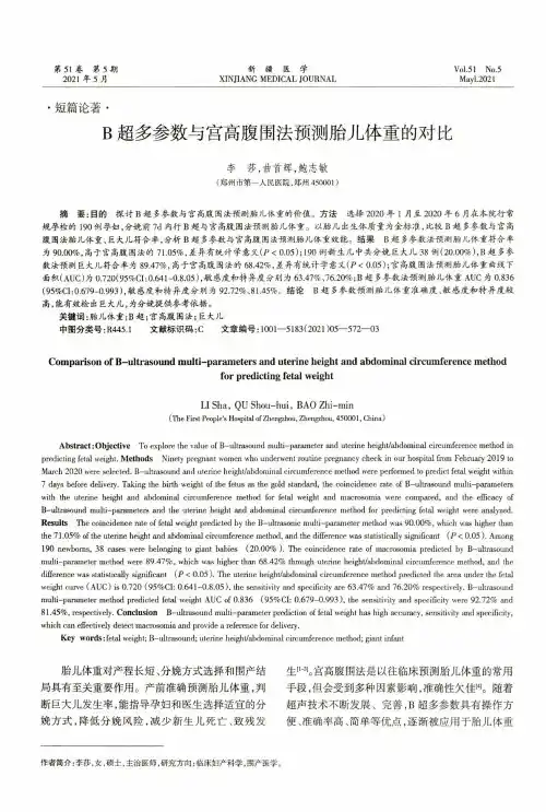
.综述.依时ROC 分析方法学综述中国医学科学院基础医学研究所/北京协和医学院基础学院统计学教研室(100005)王子兴申郁冰姜晶梅△【中图分类号】R195.1【文献标识码】A 医学中常常需要评价某种标志物、影像指标或评 分工具对疾病发生、诊断和预后的预测性能[1]。
受试者工作特征(receiver operating characteristics , ROC )曲线分析是面向上述研究目标的一类统计学方法,其基 于“金标准”将疾病状态进行二分类,进而综合分析待 评价指标各阈值所对应的灵敏度、特异度信息。
然而疾病状态与时间有关,可经历“从无到有”的变化过 程[2] 。
这种依时间而改变的结局变量给预测性能的 评价带来两方面问题:①基于不同时间截面的分析会有不同的疾病状态分布;②疾病状态可发生删失,且删 失比例随研究时间的延长而增高[3-4]。
为实现对该类 含删失的时间-状态数据的预测性能评价,经典ROC曲线和生存分析方法进行结合产生了依时ROC( time dependent ROC)分析方法[5]。
依时ROC 在过去20年内得到了极为迅速的丰富和发展,并应用于疾病预防、药物治疗等领域。
*基金项目:中国医学科学院医学与健康科技创新工程(2017-I0M-1- 009)△通信作者:姜晶梅,E-mail : jingmeijiang@ ibms. pumc. edu. cn本文从非参、半参角度总结依时ROC 分析的方法 学研究及其对应的软件实现方式,以便增进读者对依 时ROC 方法的了解并在临床转化中的应用提供参考。
基本定义1.病例和对照的三种定义依时ROC 除标志物X 阈值c 夕卜,还需结合时间阈值r 进行分析(图1),由此产生三种依时ROC 的“病 例” 和 “ 对 照 ” 定 义, 这 些 定 义 最 早 由 Heagerty 和 Zheng 于2005年总结⑷并得以沿用。
标志物取值图1依时ROC 三种定义示意图累积/动态(cumulative/dynamic , CD )定义下,累DOI 10. 3969/j. issn. 1002 - 3674. 2020.06.038积病例为研究起始点到r 时刻期间经历事件的个体(图1中的A 、B 和E ),动态对照为r 时刻仍未发生事 件的个体(图1中C 和F )。
专业术语、缩略语中英对照表缩略语英文全称中文全称ABE Average Bioequivalence 平均生物等效性AC Active control 阳性对照ADE Adverse Drug Event 药物不良事件ADR Adverse Drug Reaction 药物不良反应AE Adverse Event 不良事件AI Assistant Investigator 助理研究者ALB Albumin 白蛋白ALD Approximate Lethal Dose 近似致死剂量ALP Alkaline phosphatase 碱性磷酸酶ALT Alanine aminotransferase 丙氨酸转氨酶ANDA Abbreviated New Drug Application 简化新药申请ANOV A Analysis of variance 方差分析AST Aspartate aminotransferase 天冬氨酸转氨酶ATR Attenuated total reflection 衰减全反射法BA Bioavailability 生物利用度BE Bioequivalence 生物等效性BMI Body Mass Index 体质指数BUN Blood urea nitrogen 血尿素氮CATD Computer-assisted trial design 计算机辅助试验设计CDER Center of Drug Evaluation and Research 药品评价和研究中心CFR Code of Federal Regulation 美国联邦法规CI Co-Investigator 合作研究者CI Confidence Interval 可信区间COI Coordinating Investigator 协调研究者CRC Clinical Research Coordinator 临床研究协调者CRF Case Report/Record Form 病历报告表/病例记录表CRO Contract Research Organization 合同研究组织CSA Clinical Study Application 临床研究申请CTA Clinical Trial Application 临床试验申请CTP Clinical Trial Protocol 临床试验方案CTR Clinical Trial Report 临床试验报告CTX Clinical Trial Exemption 临床试验免责CHMP Committee for Medicinal 人用药委会Products for Human UseDSC Differential scanning 差示扫描热量计DSMB Data Safety and monitoring Board 数据安全及监控委员会EDC Electronic Data Capture 电子数据采集系统EDP Electronic Data Processing 电子数据处理系统EWP Europe Working Party 欧洲工作组FDA Food and Drug Administration 美国食品与药品管理局FR Final Report 总结报告GCP Good Clinical Practice 药物临床试验质量管理规范GCP Good Laboratory Practice 药物非临床试验质量管理规范GLU Glucose 葡萄糖GMP Good Manufacturing Practice 药品生产质量管理规范HEV Health economic evaluation 健康经济学评价IB Investigator’s Brochure研究者手册IBE IndividualBioequivalence 个体生物等效性IC Informed Consent 知情同意ICF Informed Consent Form 知情同意书ICH International Conference on Harmonization 国际协调会议IDM Independent Data Monitoring 独立数据监察IDMC Independent Data Monitoring Committee 独立数据监察委员会IEC Independent Ethics Committee 独立伦理委员会IND Investigational New Drug 新药临床研究IRB Institutional Review Board 机构审查委员会ITT Intention-to –treat 意向性分析IVD In Vitro Diagnostic 体外诊断IVRS Interactive Voice Response System 互动语音应答系统LD50 Medial lethal dose 半数致死剂量LLOQ Lower Limit of quantitation 定量下限LOCF Last observation carry forward 最接近一次观察的结转LOQ Limit of Quantitation 检测限MA Marketing Approval/Authorization 上市许可证MCA Medicines Control Agency 英国药品监督局MHW Ministry of Health and Welfare 日本卫生福利部MRT Mean residence time 平均滞留时间MTD Maximum Tolerated Dose 最大耐受剂量ND Not detectable 无法定量NDA New Drug Application 新药申请NEC New Drug Entity 新化学实体NIH National Institutes of Health 国家卫生研究所(美国)NMR Nuclear Magnetic Resonance 核磁共振PD Pharmacodynamics 药效动力学PI Principal Investigator 主要研究者PK Pharmacokinetics 药物动力学PL Product License 产品许可证PMA Pre-market Approval (Application) 上市前许可(申请)PP Per protocol 符合方案集PSI Statisticians in the Pharmaceutical Industry 制药业统计学家协会QA Quality Assurance 质量保证QAU Quality Assurance Unit 质量保证部门QC Quality Control 质量控制QWP Quality Working Party 质量工作组RA Regulatory Authorities 监督管理部门REV Revision 修订SA Site Assessment 现场评估SAE Serious Adverse Event 严重不良事件SAP Statistical Analysis Plan 统计分析计划SAR Serious Adverse Reaction 严重不良反应SD Source Data/Document 原始数据/文件SD Subject Diary 受试者日记SDV Source Data Verification 原始数据核准SEL Subject Enrollment Log 受试者入选表SFDA State Food and Drug Administration 国家食品药品监督管理局SI Sponsor-Investigator 申办研究者SI Sub-investigator 助理研究者SIC Subject Identification Code 受试者识别代码SOP Standard Operating Procedure 标准操作规程SPL Study Personnel List 研究人员名单SSL Subject Screening Log 受试者筛选表T&R Test and Reference Product 受试和参比试剂T-BIL Total Bilirubin 总胆红素T-CHO Total Cholesterol 总胆固醇TG Thromboglobulin 血小板球蛋白Tmax Time of maximum concentration 达峰时间TP Total proteinum 总蛋白UAE Unexpected Adverse Event 预料外不良事件WHO World Health Organization 世界卫生组织WHO- WHO International Conference WHO 国际药品管理当局会议ICDR A of Drug Regulatory AuthoritiesAberrant result 异常结果Absorption phase 吸收相Absorption 吸收Accuracy 准确度Accurate 精密度Administer 给药Amendment修正案Approval 批准Assess 估计Audit Report 稽查报告Audit 稽查Auditor 稽查员Analytical run/batch:分析批Benefit 获益Bias 偏性,偏倚Bioequivalence 生物等效Biosimilar /Follow-on biologics 生物仿制药Blank Control 空白对照Blind codes 编制盲底Blind review 盲态检查/盲态审核Blinding method 盲法Blinding/masking 盲法/设盲Block size 每段的长度Block 层/分段BCS 生物药剂学分类系统Carryover effect 延滞效应Case history 病历Clinical equivalence 临床等效性Clinical study 临床研究Clinical Trial Report 临床试验报告Comparison 对照Compensation 补偿,赔偿金Compliance 依从性Concomitant 伴随的Conduct 行为Confidence level 置信水平Consistency test 一致性检验Contract/ agreement 协议/合同Control group 对照组Coordinating Committee 协调委员会Crossover design 交叉设计Cross-over Study 交叉研究Cure 痊愈Data management 数据管理Descriptive statistical analysis 描述性统计分析Dichotomies 二分类Dispense 分布Diviation 偏差Documentation 记录/文件Dosage forms 剂型Dose dumping 剂量倾卸(药物迅速释放入血而达到危险浓度)Dose-reaction relation 剂量-反应关系Double blinding 双盲Double dummy 双模Drop out 脱落Effectiveness 疗效Elimination phase 消除相Emergency envelope 应急信件Enantiomers 对映体End point 终点Endpoint criteria/ measurement 终点指标Enterohepatic recycling 肠肝循环Essential Documentation 必需文件Ethical 伦理的Ethics committee 伦理委员会Evaluate 评估Exclusion Criteria 排除标准Excretion 排泄Expedite 促进Extrapolated 外推的Essentially similar product:基本相似药物Factorial design 析因设计Failure 无效,失败Finacing 财务,资金Final point 终点First pass metabolism 首过代谢Fixed-dose procedure 固定剂量法Full analysis set 全分析集GC-FTIR 气相色谱-傅利叶红外联用GC-MS 气相色谱-质谱联用Generic drug 通用名药Gene mutation 基因突变Genotoxicity tests 生殖毒性试验Global assessment variable 全局评价变量Group sequential design 成组序贯设计Hypothesis test 假设检验Highly permeable:高渗透性Highly soluble:高溶解度Highly variable drug:高变异性药物Highly:Variable Drug 高变异性药物HVDP:高变异药物制剂Identification 鉴别,身份证Improvement 好转In vitro 体外In vivo 体内Inclusion Criteria 入选表准Information Gathering 信息收集Initial Meeting 启动会议Inspection 检察/视察Institution Inspection 机构检察Instruction 指令,说明Integrity 完整,正直Intercurrent 中间发生的,间发的Inter-individual variability 个体间变异性Interim analysis 期中分析Investigational Product 试验药物Investigator 研究者Involve 引起,包括IR 红外吸收光谱Innovator Product:原创药Ka 吸收速率常LC-MS 液相色谱-质谱联用logarithmic transformation 对数转换Logic check 逻辑检查Lost of follow up 失访Mask 面具,掩饰Matched pair 匹配配对Metabolism 代谢Missing value 缺失值Mixed effect model 混合效应模式Modified release products 改良释放剂型Monitor 监查员Monitoring Plan 监察计划Monitoring Report 监察报告MS-MS 质谱-质谱联用Multi-center Trial 多中心试验Negative 阴性,否定的Non-clinical Study 非临床研究Non-inferiority 非劣效性Non-Linear Pharmacokinetics 非线性药代动力学Non-parametric statistics 非参数统计方法NTID:窄治疗指数制剂Obedience 依从性Open-blinding 非盲Open-label 非盲Original Medical Record 原始医疗记录Outcome Assessment 结果评价Outcome measurement 结果指标Outlier 离群值OIP 经口服吸收药物Parallel group design 平行组设计Parameter estimation 参数估计Parametric statistics 参数统计方法Patient file 病人档案Patient History 病历Per protocol,PP 符合方案集Permeability 渗透性Pharmacodynamic characteristics 药效学特征Pharmacokinetic characteristics 药代学特征Placebo Control 安慰剂对照Placebo 安慰剂Polytomies 多分类Post-dosing postures 给药后坐姿Potential 潜在的Power 检验效能Precision 精密度Preclinical Study 临床前研究Precursor 母体前体Premature 过早的,早发Primary endpoint 主要终点Primary variable 主要变量Prodrug 药物前体Protocol amendment 方案补正Protocol Amendments 修正案Protocol 试验方案Quality Control Sample:质控样品Rapidly dissolving:快速溶出Racemates 外消旋物Randomization 随机/随机化Range check 范围检Rating scale 量表Recruit 招募,新会员Replication 可重复Retrieval 取回,补修Revise 修正Risk 风险Run in 准备期Safety evaluation 安全性评价Safety set 安全性评价的数据集Sample Size 样本量、样本大小Sampling schedules 采血计划Scale of ordered categorical ratings 有序分类指标Secondary variable 次要变量Sequence 试验次序Seriousness 严重性Severity 严重程度Significant level 检验水准Simple randomization 简单随机Single Blinding 单盲Site audit 试验机构稽查Solubility 溶解度Specificity 特异性Specify 叙述,说明Sponsor-investigator 申办研究者Standard curve 标准曲线Statistical model 统计模型Statistical tables 统计分析表Steady state 稳态Storage 储存Stratified 分层Study Audit 研究稽查Study Site 研究中心Subgroup 亚组Sub-investigator 助理研究者Subject Enrollment Log 受试者入选表Subject Enrollment 受试者入选Subject Identification Code List 受试者识别代码表Subject Recruitment 受试者招募Subject Screening Log 受试者筛选表Subject 受试者Submit 交付,委托Superiority 检验Supplemental 增补的Supra-bioavailability 超生物利用度(试验药的生物利用度大于对照药)Survival analysis 生存分析System Audit 系统稽查SmPC:药品说明书Standard Sample:标准样品Target variable 目标变量Treatment group 试验组Trial error 试验误差Trial Initial Meeting 试验启动会议Trial Master File 试验总档案Trial Objective 试验目的Trial site 试验场所Triple Blinding 三盲Two one-side test 双单侧检验Therapeutic equivalence:治疗等效性Un-blinding 破盲/揭盲Verify 查证、核实Visual analogy scale 直观类比打分法Vulnerable subject 弱势受试者Wash-out Period 洗脱期Well-being 福利,健康Withdraw 撤回,取消药代动力学参数Ae(0-t):给药到t时尿中排泄的累计原形药。
·9CHINESE JOURNAL OF CT AND MRI, DEC. 2022, Vol.20, No.12 Total No.158【第一作者】曹红举,男,医师,主要研究方向:神经系统疾病影像学诊断方面。
E-mail:**************************【通讯作者】曹红举Different CT Perfusion Parameters in the Diagnosis and Prognosis of Acute Cerebral InfarctionCAO Hong-ju *,JIA Zhao-gang,SUN Li-na.Medical imaging department,Characteristic medical center of the Chinese people's Armed Police Force,Tianjin 300162,ChinaABSTRACT 脑梗死又被称为缺血性脑卒中,约占脑卒中患者的60%~80%,其主要是由于脑供血不足导致的脑部缺血或缺氧,是导致脑卒中患者死亡的主要原因之一[1]。
临床上治疗急性脑梗死是主要是针对于缺血半暗带区域进行干预,研究发现对于脑梗死、特别是急性脑梗死患者而言,及时进行干预和治疗对改善其预后,降低病死率等至关重要,因此早期诊断意义重大[2-3]。
电子计算机断层扫描(computed tomography,CT)是临床上对脑梗死患者常用的影像学技术,但是由于脑梗死患者早期脑组织尚未发生变化,常规CT检查往往无法观察到病灶,因而不能对脑梗死做出早期诊断[4]。
CT灌注成像(computed tomography perfusion imaging,CTP)不同于常规的CT扫描,它可以观察到急性脑梗死的病灶情况,并可以检测其相关的血流动力学变化,且具有扫描速度快,检查时间短等优点[5]。
因此,本文以我院2018年1月至2020年1月收治的急性脑梗死患者为研究对象,回顾性分析患者的影像资料,分析CTP在急性脑梗死上的诊断价值和其对患者预后的预测价值,以期为CTP在急性脑梗死患者中诊断和预后评估提供参考。
诊断试验与ROC曲线分析目录一、基本概念1.诊断试验四格表基本统计基本指标2.ROC曲线:二、实例分析1)各诊断项目(变量)分别诊断效果分析:2)诊断模型分析:3)比较两预测模型:4)时间依赖的ROC曲线(Time-dependent ROC)分析一、基本概念1.诊断试验四格表基本统计基本指标诊断试验金标准诊断结果合计患病(D+)未患病(D-)阳性a(真阳性)b(假阳性)a+b阴性c(假阴性)d(真阴性)c+d合计a+c b+d N=a+b+c+d1)检测患病率(prevalence): 是指被检测的全部对象中,检测出来的患者的比例。
即:检测患病率 = (a+b)/(a+b+c+d)2)实际患病率(prevalence): 是指被检测的全部对象中,真正患者的比例。
即:实际患病率 = (a+c)/( a+b+c+d)。
实际患病率对被评价的诊断试验也称为验前概率,而预测值属于验后概率。
3)敏感性: 敏感性就是指由金标准确诊有病组内所检测出阳性病例数的比率(%)。
即本实验诊断的真阳性率。
其敏感性越高,漏诊的机会就越少。
即:敏感性= a/( a+c)4)特异性: 是指由金标准确诊为无病组内所检测出阴性人数的比率(%),即本诊断实验的真阴性率。
特异性越高,发生误诊的机会就越少。
即:特异性= d/(b+d)5)诊断准确率: 是指临床诊断检测出的真阳性和真阴性例数之和,占总检测人数的比例,即称本临床实验诊断的准确性。
即:准确性= (a+d)/ (a+b+c+d)6)阳性似然比(positive likelihood ratio): 阳性似然比是指临床诊断检测出的真阳性率与假阳性率之间的比值,即阳性似然比=敏感性/(1-特异性)= (a/(a+c))/(b/(b+d))。
可用以描述诊断试验阳性时,患病与不患病的机会比。
提示正确判断为阳性的可能性是错误判断为阳性的可能性的倍数。
阳性似然比数值越大,提示能够确诊患有该病的可能性越大。
计量经济学英汉术语名词对照及解释A校正R2(Adjusted R-Squared):多元回归分析中拟合优度的量度,在估计误差的方差时对添加的解释变量用一个自由度来调整。
对立假设(Alternative Hypothesis):检验虚拟假设时的相对假设。
AR(1)序列相关(AR(1) Serial Correlation):时间序列回归模型中的误差遵循AR(1)模型。
渐近置信区间(Asymptotic Confidence Interval):大样本容量下近似成立的置信区间。
渐近正态性(Asymptotic Normality):适当正态化后样本分布收敛到标准正态分布的估计量。
渐近性质(Asymptotic Properties):当样本容量无限增长时适用的估计量和检验统计量性质。
渐近标准误(Asymptotic Standard Error):大样本下生效的标准误。
渐近t 统计量(Asymptotic t Statistic):大样本下近似服从标准正态分布的t统计量。
渐近方差(Asymptotic Variance):为了获得渐近标准正态分布,我们必须用以除估计量的平方值。
渐近有效(Asymptotically Effcient):对于服从渐近正态分布的一致性估计量,有最小渐近方差的估计量。
渐近不相关(Asymptotically Uncorrelated):时间序列过程中,随着两个时点上的随机变量的时间间隔增加,它们之间的相关趋于零。
衰减偏误(Attenuation Bias):总是朝向零的估计量偏误,因而有衰减偏误的估计量的期望值小于参数的绝对值。
自回归条件异方差性(Autoregressive Conditional Heteroskedasticity, ARCH):动态异方差性模型,即给定过去信息,误差项的方差线性依赖于过去的误差的平方。
一阶自回归过程[AR(1)](Autoregressive Process of Order One [AR(1)]):一个时间序列模型,其当前值线性依赖于最近的值加上一个无法预测的扰动。
estimation可以用作名词和动词,当用作名词时,它的意思是“估计;预估;判断;看法”,可以用作不可数名词。
estimation也可用作动词,意思是“估计;估价;评估”,一般用复数形式。
estimation的用法举例如下:
1. We can only give a rough estimation of the cost. 我们只能对费用做一个大致的估算。
2. They will have to make a careful estimation of the cost. 他们将不得不仔细估算成本。
3. The government has given a cautious estimation of the damage caused by the earthquake. 政府对地震造成的损失做了一个谨慎的估算。
4. The government's estimation of the cost was based on the best available evidence. 政府对成本的估算基于现有最确凿的证据。
希望以上信息对你有帮助。
Biometrics59,614–623September2003Partial AUC Estimation and RegressionLori E.Dodd1,∗and Margaret S.Pepe2,∗∗1Biometric Research Branch,National Cancer Institute,6130Executive Blvd,MSC7434,Rockville,Maryland20892,U.S.A.2Department of Biostatistics,University of Washington,Box357232,Seattle,Washington98195,U.S.A.∗email:doddl@∗∗email:mspepe@Summary.Accurate diagnosis of disease is a critical part of health care.New diagnostic and screening tests must be evaluated based on their abilities to discriminate diseased from nondiseased states.The partial area under the receiver operating characteristic(ROC)curve is a measure of diagnostic test accuracy.We present an interpretation of the partial area under the curve(AUC),which gives rise to a nonparametric estimator.This estimator is more robust than existing estimators,which make parametric assumptions.We show that the robustness is gained with only a moderate loss in efficiency.We describe a regression modeling frameworkfor making inference about covariate effects on the partial AUC.Such models can refine knowledge about test accuracy.Model parameters can be estimated using binary regression methods.We use the regression framework to compare two prostate-specific antigen biomarkers and to evaluate the dependence of biomarker accuracy on the time prior to clinical diagnosis of prostate cancer.Key words:Diagnostic testing;Mann-Whitney U-statistic;Regression;Receiver operating characteristic curve.1.IntroductionScreening and diagnostic tests are familiar and ever-evolvingtools of modern medicine.Populations of healthy individu-als characterized as at-risk are commonly screened for dis-eases such as cancer and heart disease.Early detection byscreening is considered essential to alleviate disease burden,and considerable resources have been devoted to developingnew screening tests.New diagnostic tests that are less inva-sive,less expensive,and more accurate than existing proce-dures are sought for diagnosis of many conditions.Technolo-gies that measure gene and protein expression,as well as newimaging procedures,all hold promise in this regard.Prior towidespread application,however,rigorous evaluation of testaccuracy and of factors that effect it is compulsory.Inherent in the analysis of screening and diagnostic tests arecosts and benefits,both monetary and nonmonetary,associ-ated with true-positive and false-positive diagnoses.Considera continuous test result Y for which Y>c indicates a positivetest result,and let D and¯D denote diseased and nondiseasedstates,respectively.The true-positive rate at a threshold c,TPR(c),is defined as P(Y>c|D)≡S D(c).The correspondingfalse-positive rate,FPR(c),is P(Y>c|¯D)≡S¯D(c).Costsand benefits are associated with any given{FPR(c),TPR(c)}pair.The receiver operating characteristic(ROC)curve plots{FPR(c),TPR(c)}for all possible thresholds c,and providesa visual description of the trade-offs between TPRs and FPRsas one changes the threshold stringency(Figure1).We canwrite the ROC curve as a function of t=S¯D(c)as follows:ROC(t)=S D{S−1¯D (t)}.An uninformative test is representedby a straight line from the(0,0)vertex to(1,1),while acurve pulled closer towards the(0,1)vertex indicates a better-performing test.Frequently,the best threshold is not known when a test isunder evaluation,and it may vary depending on the settingin which the test is implemented.A summary measure thataggregates performance information across a range of pos-sible thresholds is desirable.The area under the ROC curve(AUC),defined as1ROC(t)dt,summarizes across all thresh-olds,and is the most commonly used measure of diagnosticaccuracy for quantitative tests.However,the AUC summa-rizes test performance over regions of the ROC space in whichone would never operate,i.e.,for{FPR(c),TPR(c)}values ofno practical interest.In population screening,large monetarycosts result from high false-positive rates;hence the region ofthe curve corresponding to low false-positive rates is of pri-mary interest.In diagnostic testing,it is critical to maintaina high TPR in order not to miss detecting subjects with dis-ease.In this case,interest is in the region of the ROC curvecorresponding only to acceptably high TPRs.In this article,we consider a summary index for the ROC curve restricted toa clinically relevant range of false-positive rates.The partialAUC isAUC(t0,t1)=t1t0ROC(t)dt,(1)where the interval(t0,t1)denotes the false-positive rates of in-terest.The analogue that restricts to a range of true-positiverates will also be discussed.Selecting the interval(t0,t1)is an614Partial AUC Estimation and Regression615 important practical issue.The choice depends on the particu-lar setting and should depend on the costs of a false-positivediagnosis,as well as the benefits of a true positive.Baker(2000)develops a“utility”function to specify a target par-tial ROC region.Obuchowski(1997)uses decision analysis toassociate patient outcome with desirable diagnostic accuracyvalues.Such methods could be adapted,for example,to de-termine a maximum allowable false-positive rate or the lowestdesirable true-positive rate.This is a complex area requiringinput from health services and economic specialists.Although the partial AUC has been proposed before(McClish,1989;Thompson and Zucchini,1989;Jiang,Metz,and Nishikawa,1996)and has gained popularity,particularlyin screening research(Baker and Pinsky,2001),little attentionhas been devoted to statistical inference about it.We providea probabilistic interpretation for the partial AUC that givesrise to a novel nonparametric estimator.Through simulationstudies,the estimator is compared with the existing estima-tors that are all based on parametric assumptions.We showthat the increased robustness of the nonparametric estima-tor is gained at the expense of a moderate loss in efficiency.Then we present a regression framework for evaluating co-variate effects on the partial AUC.The approach extends amethod developed recently for regression analysis of the fullAUC(Dodd and Pepe,2003).Since the partial AUC has moreappeal in many practical settings,this represents an impor-tant generalization.The work is motivated by a study of prostate-specific anti-gen(PSA),a serum biomarker.PSA is a screening tool forprostate cancer that has been the focus of much research.Im-portant questions to consider when evaluating this biomarkerare,which form of PSA is best(total or ratio of free to totalPSA),and by how long does this test advance the lead time,or time prior to clinical diagnosis of disease?In this article,we show that a parsimonious regression model of the partialAUC with PSA type,and lead time as covariates,assists withthis type of evaluation.2.Partial AUCThe partial AUC is simply the area under the ROC curvebetween t0and t1(Figure1).With an uninformative test,TPR(c)=FPR(c)for all c,and the partial AUC is the areaof a trapezoid equal to1/2(t1+t0)(t1−t0).For a perfect test,ROC(t)=1for all t∈(0,1),and the partial AUC is the areaof the rectangle with height1and base t1−t0.2.1Interpretations of the Partial AUCAssume Y D and Y¯D are continuous random variables withsurvivor functions S D and S¯D,respectively.Let F=1−S.The partial AUC is the joint probability that Y D>Y¯D andthat Y¯D falls within the range of clinically relevant quantiles.To see this,observe that:AUC(t0,t1)=t1t0ROC(t)dt=t1t0S DS−1¯D(t)dt=S−1¯D(t0)S−1¯D(t1)S D(y)dF¯D(y)FPRTPR0.00.20.40.60.8 1.01Figure1.Illustration of an ROC curve and its partial AUC(t0=0.1,t1=0.3).=S−1¯D(t0)S−1¯D(t1)S D(y)f¯D(y)dy=PY D>Y¯D,Y¯D∈S−1¯D(t1),S−1¯D(t0)(2)To simplify notation let q0=S−1¯D(t0)and q1=S−1¯D(t1).Thepartial AUC can also be written as a weighted conditionalexpectation AUC(t0,t1)=(t1−t0)P{Y D>Y¯D|Y¯D∈(q1,q0)}.A second interpretation arises from the concept of place-ment values(Pepe,2003).The term S D(y¯D)is the placementof a given nondiseased test result,Y¯D=y¯D,in the survivorfunction of results of diseased.For a good test,the nondis-eased observations fall in the lower tail of the distributionof diseased.Hence,larger placement values indicate a bettertest.Hanley and Hajian-Tilaki(1997)showed a connectionbetween average placement values and the full AUC.We ex-tend their result to the partial AUC here,as it provides aninteresting interpretation of the partial AUC,as well as a sim-pler estimator:P{Y D>Y¯D,Y¯D∈(q1,q0)|Y¯D=y¯D}=P{Y D>y¯D,y¯D∈(q1,q0)}=I{y¯D∈(q1,q0)}P(Y D>y¯D)=I{y¯D∈(q1,q0)}S D(y¯D)≡Pl D(y¯D)(3)We refer to Pl D(y¯D)as a“restricted placement value”(withrespect to the distribution of results from the diseased pop-ulation).Note that a full placement value is defined as in(3),except there is no restriction to Y¯D∈(q0,q1).The re-stricted placement is weighted so that only those values thatfall within the relevant quantiles are considered.Note thatE{Pl D(Y¯D)}=AUC(t0,t1).Thus,the partial AUC can bethought of as an average of restricted placement values.It616Biometrics,September2003 is straightforward to show that the partial AUC is also theexpected restricted placement value from conditioning on ob-servations from the diseased population.One may wish to rescale the partial AUC,especially inregression analysis(see Section5).We define the partial AUCodds asAUC(t0,t1)/{(t1−t0)−AUC(t0,t1)}=P{Y D>Y¯D|Y¯D∈(q1,q0)}/P{Y D<Y¯D|Y¯D∈(q1,q0)}.(4) This is the ratio of the probability of a correct ordering ofa randomly selected diseased and nondiseased test result tothe probability of an incorrect ordering,with both probabili-ties conditional on the test result of nondiseased arising fromthe region of interest.These odds have value of(t1+t0)/{2−(t1+t0)}when a test is uninformative,and of infinityfor a perfect test.2.2Restricting the True-Positive RangeThe partial AUC just described restricts the ROC region ofinterest to false-positive rates that take values in(t0,t1).Insome settings,one may wish to restrict to a range of true-positive rates(Jiang et al.,1996).By transforming the ROCcurve to a plot of{S D(c),1−S¯D(c)},interpretations of a par-tial AUC corresponding to true-positive rates in an intervalare easily obtained.The curve is no longer the classic ROCcurve.It is simply a270◦rotation of Figure1.We refer to thiscurve as the specificity-ROC curve(ROC spe),since specificityis plotted on the y-axis.For u=S D(c),this curve is describedby ROC spe(u)=1−S¯D{S−1D(u)}=F¯D{S−1D(u)}.The partialAUC for a range of true positives,denoted AUC TP(u0,u1),isdefined asu1u0ROC spe(u)du=S−1D(u1)S−1D(u0){1−S¯D(y)}dS D(y)=PY D>Y¯D,Y D∈S−1D(u1),S−1D(u0).(5)Note that1S D(y)dS¯D(y)=1{1−S¯D(y)}dS D(y).Therefore,the two representations give the same full AUC. However,the quantiles that define the partial AUC are{S−1¯D (t1),S−1¯D(t0)},and are derived from the nondiseaseddistribution for the classic ROC curve.For the case justpresented,the quantiles are{S−1D (u1),S−1D(u0)},and arisefrom the distribution of tests of diseased subjects.With this exception,the interpretations are the same.Thus,we focus on the classic ROC curve,recognizing that methods developed here easily extend to the case in which restriction of true-positive rates is required.3.Estimators3.1Parametric EstimatorsBefore proposing our nonparametric estimator,we briefly de-scribe existing estimators.McClish(1989)describes what we refer to as the normal-distributions partial AUC esti-mator(NDE),which assumes that the test results for dis-eased and nondiseased populations follow normal distribu-tions with different means and variances.Maximum likelihood estimates of these parameters provide the ROC curve esti-mate,and numerical integration of it gives the partial AUC es-timator:AUC(t0,t1)=t1t0Φ{ˆa+ˆbΦ−1(t)}dt.HereΦdenotes the standard normal cumulative distribution function(CDF),ˆa=(ˆµD−ˆµ¯D)/ˆσD andˆb=ˆσ¯D/ˆσD,whereµandσ2denote mean and variance,respectively.Another approach is to parameterize the ROC curve di-rectly.The most common form is the binormal ROC curve, ROC(t)=Φ{a+bΦ−1(t)},for which the partial AUC is given by the same formula above.However,because this approach does not parameterize the distributions of test results,but only the ROC curve that describes the relationship between their distributions,it stipulates far weaker assumptions.Two methods have been proposed for estimating parameters a and b of the binormal ROC curve(Metz,Herman,and Shen,1998; Pepe,2000).Both methods are distribution-free in that they are functions only of the ranks of the data.3.2Proposed Nonparametric EstimatorDenote V q0,q1ij=I{Y D i>Y¯D j,Y¯D j∈(q1,q0)}and observethat E(V q0,q1ij)=P{Y D>Y¯D,Y¯D∈(q1,q0)}=AUC(t0,t1), according to the interpretation of equation(1).This suggests the following method-of-moments estimator:AUC(t0,t1)=(n D n¯D)−1ijV q0,q1ij,(6)where n D and n¯D denote the number of observations from the population of diseased and nondiseased,respectively.In some circumstances,the quantiles(q0,q1)will be known. In others,they will not,in which case empirical quantile es-timates are substituted.If the empirical quantile value does not coincide precisely with the desired value,as may hap-pen with small sample sizes,values are linearly interpo-lated.Observe that,when t0=0and t1=1,AUC(t0,t1)= (n D n¯D)−1ijI(Y D i>Y¯D j).Hence,for the full AUC the es-timator reduces to the Mann-Whitney U-statistic,the classic nonparametric AUC estimator.Further,note that this results in the same value as the area calculated from the empirical ROC curve,using the trapezoidal rule when there are no ties in the data.The same estimator is derived by consideration of empir-ical restricted placement values.LetˆS denote an empirical survivor function and write the empirical placement value cor-responding to an observation from a disease-free subject,Y¯D, as:Pl D(Y¯Dj)=IY¯D j∈(q1,q0)ˆSDY¯D j=IY¯D j∈(q1,q0)(1/n D)n DiIY D i>Y¯D j.(7) The sample average is(1/n¯D)n¯DjPl D Y¯Dj=(n D n¯D)−1n¯Djn DiIY D i>Y¯D j,Y¯D j∈(q1,q0).Partial AUC Estimation and Regression617Thus,the nonparametric estimator is an average of restricted placement values within the disease reference distribution.Likewise,the estimator can be written as the average of the placement values within the nondiseased reference distribu-tion.This generalizes the corresponding results for the full AUC given in DeLong,DeLong,and Clarke-Pearson (1988)and Hanley and Hajian-Tilaki (1997).Calculations using placement values are considerably faster computationally,and are used in the simulations described next.Asymptotic distribution theory is nonstandard because thebinary indicators,V q 0,q 1ij,are cross-correlated.It can be shown that the projection (n D n ¯D )−1ijPl ¯D (Y D i )+Pl D (Y ¯D j )is asymptotically equivalent to (6).Since this projection is a sum of independent terms,standard theory provides consis-tency and asymptotic normality results.For complete details,refer to Dodd (2001).We recommend using the bootstrap to obtain variance estimates.4.Simulations4.1Small Sample Performance of the EstimatorThree different ROC models were simulated to evaluate per-formance of the proposed method of inference.The models simulated are a normal-distributions model,a proportional-hazards ROC model,and an extreme-value ROC model.The proportional-hazards ROC model assumes that the hazard function for the disease test result distribution is proportional to that of the nondisease distribution.If the ratio of hazards is r ,then ROC(t )=t r .The extreme-value ROC model in-volves two parameters (e ,f ),and is of the form ROC(t )=exp[−(1/e )exp {−f Φ−1(t )}](Cai and Pepe,2003).Extensive simulations of these models described in Dodd (2001)showed that the nonparametric method produced estimates with little bias and that confidence intervals using the bootstrap stan-dard error estimator and normal quantiles provided good cov-erage probability.We present results for a normal-distributions modelthat assumes Y D ∼N (1.5, 1.44)and Y ¯D ∼N (0,1)(see Figure 1).Partial AUCs are considered for (t 0,t 1)={(0,0.1),(0,0.2),(0.1,0.2),(0.1,0.3)}when quantiles are both known and estimated empirically.Sample sizes were gener-ated with both equal and unequal numbers in each group,such that (n D ,n ¯D )={(10,50),(10,100),(50,50),(50,100),(100,100),(100,200),(100,300)}.All resulted in estimates with little bias (Table 1).The largest amount of bias (5.4%)occurs for n D =10and n ¯D =50,for (t 0,t 1)=(0.1,0.2),when known quantiles are used.Bias becomes negligible as sample size increases and as more of the curve is integrated.In most cases,bootstrapped standard errors,computed with 200bootstrap samples,slightly overestimate the truth when the quantiles are estimated.In the case when quantiles are known,the bootstrapped standard error estimator is rea-sonably unbiased.Consequently,confidence interval coverage tends to be above the nominal level with estimated quantile values,but close to the nominal level with the known thresh-old.Surprisingly,when empirical quantiles are substituted,there is an increase in efficiency compared to the case when the true quantile is used.The true standard errors associatedwith AUC {t 0(ˆq ),t 1(ˆq )}are consistently smaller than those for AUC{t 0(q ),t 1(q )}.The reason for this is unclear to us,but it is a real phenomenon observed throughout our simulation stud-ies.Simulations suggest that the empirical quantile estimatoris negatively correlated with the partial AUC estimator,hence reducing the variance.However,explicit characterization of this correlation is difficult to obtain.4.2RobustnessTo investigate if the nonparametric estimator gains robust-ness over other estimators,we considered settings where the ROC curve deviated from the classic binormal form.We gen-erate an ROC model in which test results arise from mixturesof distributions.Assume that Y ¯D ∼N (0,1),but that Y D is a mixture of two normal distributions,f Z 1and f Z 2,with Z 1∼N (µD,1,σ2D,1)and Z 2∼N (µD,2,σ2D,2),such that the prob-ability density of Y D is p f Z 1(y )+(1−p )f Z 2(y ),for a mixing proportion p ∈(0,1).The resulting ROC curve is simply a mixture of ROC curves weighted by the appropri-ate mixing probabilities and can be expressed as ROC(t )=p Φ{a 1+b 1Φ−1(t )}+(1−p )Φ{a 2+b 2Φ−1(t )},where a i =(µD,i −µ¯D,i )/(σD,i )and b i =σ¯D,i /σD,i for i =1,2.We setµD 1=5,σ2D 1=1.2,µD 2=0,σ2D 2=1,and p =0.3.The true ROC curve is the solid line shown in Figure 2.We use t 0=0and three separate maximum false-positive rates,t 1=0.05,0.1,1.0.Very low false-positive rates,such as t 1=0.05,have been advocated in settings such as cancer screening (Baker and Pinsky,2001).Estimates of ROC curves from the NDE,the Pepe esti-mator (PPE)and the Metz estimator (MZE)are also given in Figure 2.Recall that the normal-distributions estima-tor assumes that test results are normally distributed in diseased and nondiseased ing sample meansand variances,the ROC curve is calculated as ROC(t )=Φ{ˆa +ˆb Φ−1(t )}with ˆa =(ˆµD −ˆµ¯D )/ˆσD and ˆb =ˆσ¯D /ˆσD .Clearly,all of these curves fail to accurately represent the true0.00.20.40.60.8 1.0FPRT P RFigure 2.Estimates of the ROC based on data from the mixture model.Shown are curves that use the average pa-rameter estimates.618Biometrics,September2003Table1Bias and coverage probability of the nonparametric method with known and estimated quantilesAUC{t0( q),t1( q)}AUC{t0(q),t1(q)}n D n¯D Bias S E(SE)×100CP Bias S E(SE)×100CPAUC(0,0.1)=0.0421050 3.28% 1.578(1.600)0.950.71% 2.315(2.344)0.88 10100 2.11% 1.443(1.492)0.950.11% 1.971(1.905)0.93 5050 4.30%0.109(0.101)0.96 1.90%0.200(0.192)0.90 50100 2.60%0.085(0.087)0.94<0.01%0.152(0.146)0.93 100100 1.50%0.075(0.072)0.95−0.20%0.138(0.139)0.94 1002000.20%0.06(0.061)0.940.60%0.102(0.103)0.95AUC(0,0.2)=0.1071050 1.20% 2.957(2.978)0.96 2.98% 4.198(4.388)0.92 101000.58% 2.761(2.848)0.940.14% 3.557(3.347)0.93 5050 1.50%0.185(0.172)0.97 1.60%0.347(0.338)0.92 50100 1.20%0.152(0.155)0.94 1.80%0.269(0.252)0.92 1001000.80%0.128(0.127)0.94−1.40%0.224(0.237)0.96 1002000.00%0.107(0.109)0.94−0.20%0.178(0.178)0.95AUC(0.1,0.2)=0.0651050−0.17% 1.929(1.593)0.99 5.40% 3.119(3.403)0.88 10100−0.43% 1.616(1.530)0.95−0.23% 2.479(2.569)0.92 5050−0.30%0.136(0.086) 1.00 1.40%0.284(0.280)0.92 501000.40%0.094(0.080)0.98 3.00%0.217(0.203)0.92 1001000.30%0.082(0.065)0.99−2.10%0.191(0.197)0.95 100200−0.20%0.061(0.055)0.96−0.80%0.147(0.144)0.94AUC(0.1,0.3)=0.1401050−0.27% 3.113(2.877)0.96 2.01% 4.871(4.915)0.92 10100−0.30% 2.820(2.774)0.94−0.11% 3.939(4.037)0.94 5050−0.30%0.194(0.151)0.99 1.40%0.416(0.414)0.95 501000.10%0.151(0.142)0.96 1.90%0.301(0.305)0.94 1001000.30%0.126(0.114)0.97−2.10%0.281(0.293)0.95 100200−0.10%0.103(0.099)0.950.40%0.218(0.216)0.95 Note:SE is bootstrapped standard error(×100)from200bootstrap samples,SE is true standard error(×100),and CP is coverage probability for95%confidence intervals using SE with a normal quantile.Results represent1000realizations of normal-distributions model.curve,which is not of the binormal form.They parameterize the ROC curve incorrectly,and hence produce biased par-tial AUC estimates(Table2).The largest bias was observed with the normal-distributions estimator.In contrast to this estimator and those of Pepe and Metz,the nonparametric es-timators produce estimates with very small bias.Observe that the amount of bias decreases for both the Metz and the Pepe estimators as more of the curve is integrated.This is consis-tent with results showing that the binormal model estimators produce AUC estimates that are robust to departures from this model(Hanley,1996).Additionally,note that the more parametric methods model and estimate the ROC over the entire(0,1)range and then integrate the relevant portion to determine the par-tial AUC.In contrast,the proposed method directly estimates the partial AUC over the false-positive rate range of inter-est.A more robust approach might be to model over(t0,t1), which can be accommodated by the Pepe approach.When the estimates are computed while restricting to(0,0.05)and (0,0.2),however,there is still bias with the Pepe method.The mean estimates restricting to the corresponding intervals areAUC(0,0.05)=0.013(−18%bias)andAUC(0,0.2)=0.044 (−40%bias).4.3EfficiencyWe compare the efficiency of the methods for estimating the partial AUC under the normal-distributions model.In this setting,the normal-distributions estimator is more efficient than the others,as it is the maximum likelihood estimator and makes use of the information that the data are nor-mally distributed.The results presented in Figure3indi-cate that the nonparametric estimator with known quantile, NPE(q),is the least efficient of the methods.In agreement with Table1,we observe that the nonparametric estimator is more efficient when the quantile is estimated than when the known value is used.The distribution-free binormal es-timators are more efficient than the nonparametric estima-tor,but have reduced efficiency relative to the approach that models the test results.Although very similar,the Pepe es-timator appears to be slightly more efficient than the Metz estimator.The efficiency of all methods approaches that of the normal-distributions estimator as t→1.Recall that when t=1,the nonparametric estimator is the Mann-Whitney U-statistic.The normal-distributions estimator is simply a transformation of the standardized differences in means,i.e., of the Z-statistic.Hence,the comparison of the variancePartial AUC Estimation and Regression619Maximum False Positive RateR e l a t i v e E f f i c i e n c y0.00.20.40.60.8 1.0Figure 3.Efficiency of estimators relative to the maximum likelihood normal-distributions estimator.Shown are results with sample sizes of 200per group and 2000replicates per scenario.of the nonparametric estimator with the variance of the normal-distributions estimator is akin to the comparison of the efficiency of the Mann-Whitney U-statistic to that of the Z-statistic.It is well known that the asymptotic relative ef-Table 2Bias in partial AUC estimates from ROC mixture model.Shown are results with 200samples per group and 1000simulations of the model.MethodEstimatePercent biasAUC(0,0.05)=0.0158Nonparametric estimator (ˆq )0.0161Nonparametric estimator (q )0.016<1Pepe estimator 0.003−81Metz estimator 0.01222Normal-distributions estimator 0.02346AUC(0,0.2)=0.074Nonparametric estimator (ˆq )0.0751Nonparametric estimator (ˆq )0.074<1Pepe estimator 0.043−41Metz estimator 0.0785Normal-distributions estimator 0.11049AUC(0,1)=0.649Nonparametric estimator 0.651<1Pepe estimator 0.634−2Metz estimator 0.6754Normal-distributions estimator 0.7099ficiency of the Mann-Whitney U-statistic to the t-statistic is 0.95(Lehmann,1997).Thus it is no surprise that,in this study,the relative efficiency is 0.94at t =1.4.4RecommendationsThe normal-distributions estimator,while most efficient,produces unacceptably biased estimates.Estimators that pa-rameterize the ROC curve are similarly not robust.The nonparametric estimator provides substantially more robust estimation.The added robustness is at the expense of mod-erate losses in efficiency.Hence,we recommend use of the nonparametric estimator.Indeed,for partial areas with t >0.1,it has similar efficiency to the Pepe and Metz methods.5.Regression AnalysisAccuracy may depend on information other than the test re-sult itself.For example,accuracy may depend on how close in time a subject is to clinical diagnosis.Patient characteristics,such as age or family history of disease,may also be relevant determinants of accuracy.This information may guide deci-sions about what populations are most likely to benefit from testing or for what populations test innovations are needed.We extend regression methodology we previously developed for the AUC to a regression methodology for the partial AUC summary index of test accuracy.For a more extensive discus-sion of modeling approaches for the AUC and details about fitting,refer to Dodd and Pepe (2003).Here,we elaborate only on aspects unique to the partial AUC.620Biometrics,September20035.1ModelsTo assess the effect of covariates on test accuracy,we pro-pose the following partial AUC regression models.Considera vector of covariates X.Define the covariate-specific partialAUC as AUC X(t0,t1)=P{Y D>Y¯D,Y¯D∈(q0,q1)|X}.Fora specified link function g,the general model is given byAUC X(t0,t1)=g(X Tβ)(8)Possible link functions include the logit or probit forms.How-ever,since AUC(t0,t1)has an upper bound of(t1−t0),a generalization of the logit that incorporates this constraint is appropriate:g−1(u,t0,t1)=log{u/(t1−t0−u)}.When thislink is used,an interpretation that corresponds to the partialAUC odds defined earlier follows.Consider the modellog[AUC X(t0,t1)/{(t1−t0)−AUC X(t0,t1)}]=β0+β1X.(9)It follows that eβ1is a ratio of partial AUC odds for X+1to X.When eβ1>1,the partial AUC odds are an increasingfunction of X,and accuracy increases with X.If eβ1<1,thepartial AUC odds are a decreasing function of X.Refer toDodd and Pepe(2003)for details about model specification.5.2Estimating FunctionConsider the indicators V(q0,q1)ij as defined in(6),butnow we condition on the covariates X.They have meanE{V(q0,q1)ij |X}=AUC X(t0,t1),which suggests that binary re-gression methods can be used to estimate partial AUC model parameters with the following estimating equation:V nD,n¯D (β)=n Din¯Dj(∂θX/∂β)ν−1(θX)V(q0,q1)ij−θX=0.(10)Here,θX=AUC X(t0,t1),ν−1(θX)is the variance of V(q0,q1),and(∂θX/∂β)is a(p×1)vector of the partial derivatives ofθX with respect to the model parametersβ.This resemblesthe classic estimating equation for binary regression.However,the binary indicators are cross-correlated in the sense that,fora given i,the set of binary variables{V ij,j=1,...,n¯D}are correlated because they are a function of Y D i.Consistency andasymptotic normality for parameter estimates from a similarestimating equation is developed in Dodd and Pepe(2003).The same theory applies here,at least when the quantiles(q0,q1)are known.See Dodd(2001)for a full exposition.5.3Comparing Two TestsThe proposed estimating equation gives rise to astandard approach when a model to compare twotests is of interest.Consider the following model:log[AUC X(t0,t1)/{t1−t0−AUC X(t0,t1)}]=β0+β1X, where X is an indicator of test type.The scorelike test of β1=0,based on the estimating equation in(10),reduces toAUC X=1(t0,t1)−AUC X=0(t0,t1),whereAUC(t0,t1)isdefined as in(6).This statistic is a member of the familyof statistics proposed by Wieand et al.(1989)that takesintegrated differences in weighted ROC curves to comparetwo tests.The Wieand et al.approach does not requirebootstrapping for inference,as does ours when the quantiles,q0and q1,are unknown.The current approach,on the otherhand,provides a more general regression framework.5.4ImplementationTo obtain parameter estimates,algorithms developed for bi-nary regression are used.First,however,the quantiles(q0, q1)must be specified.If known,they are simply substituted into(10).If quantiles are unknown and do not depend on co-variates,they can be estimated empirically from the nondis-ease data at hand.If the unknown quantiles depend on co-variates,a quantile regression model may be specified(see Heagerty and Pepe,1999).Then,the binary indicators based on pairs of diseased and nondiseased observations are com-puted.When covariates are categorical and there are suffi-cient observations of diseased and nondiseased within each category,all possible pairs of diseased and nondiseased within a given category are created.That is,the n kDand n k¯Dobserva-tions corresponding to the category or level of covariate k areselected and we calculate V(q0,q1)ijat each X for k=1,...,K. Note that the estimating function is modified to indicate the sum over k.When covariates are continuous,pairing of dis-eased and nondiseased observations(Y D i,Y¯D j)may be under-taken for all possible pairs,although we prefer to pair those observations only with covariate values near one another.Fi-nally,if covariates are unique to the diseased group,as with the“time prior to diagnosis”covariate in the PSA example that follows,the covariate does not restrict the pairing.Pair-ing is based only on covariates common to D and¯D.We refer to the article on AUC regression by Dodd and Pepe(2003)for a detailed discussion of pairing in the presence of covariates. The same considerations are relevant here.Logistic or probit regression estimation routines in stan-dard statistical packages can be used to solve the estimat-ing equations.Note that standard errors reported from these packages will not be valid,even with a robust sandwich vari-ance estimator,because of the crossed-correlation structure. We use the bootstrap to calculate the standard errors for pa-rameter estimates.Bootstrap samples are taken by sampling subjects as the primary unit.6.Prostate-Specific Antigen AnalysisThe data analyzed here are taken from a retrospective sam-pling of stored serum from theα-Tocopherol andβ-Carotene Study(ATBC),described by Heinonen et al.(1998).Al-though the primary goal of this study was to evaluate the effect of dietary supplementation ofα-tocopherol and β-carotene on lung cancer risk,the development of prostate cancer was also recorded.Additionally,serum samples were collected and stored both at baseline and three years later. For those240subjects who were diagnosed with prostate can-cer during the eight-year follow-up period,their serum sam-ples were retrospectively evaluated for prediagnostic levels of prostate-specific antigen.Age-matched serum samples for 237non-prostate-diagnosed subjects were selected for com-parative purposes.Two ways of quantifying PSA were con-sidered,the total PSA in serum(denoted by“total”)and the ratio of free to total PSA in serum(denoted by“ratio”). Etzioni et al.(1999)previously compared these two measures using a different dataset.In addition to comparing total to ratio PSA,we examine the effect on accuracy of time from serum sampling to clinical diagnosis.One would expect that PSA levels taken close to the time of clinical time of diagnosis would be more predictive.Let“test”denote an indicator that takes a value of one for total PSA and zero for PSA ratio.。