Fully automatic modelling of cohesive discrete crack

Subject headings: black hole physics — galaxies: elliptical and lenticular, cD — galaxies: individual (NGC 4342) — galaxies: kinematics and dynamics — galaxies: nuclei — galaxies: structure.
–3– 1. Introduction
Several lines of evidence suggest that active galactic nuclei (AGNs) are powered by accretion onto a super-massive black hole (BH) (Lynden-Bell 1969; Rees 1984). The much higher volume-number density of AGNs observed at redshift z ≈ 2 than at z = 0, suggests that many quiescent (or ‘normal’) galaxies today must have gone through an active phase in the past, and therefore harbor a massive BH as well. Such a BH will significantly influence the dynamics of the galaxy inside a radius of influence, rBH = GMBH /σ 2 , where σ is a characteristic velocity dispersion of the stars in the center. In particular, hydrostatic equilibrium requires that the rms velocities of the stars surrounding a massive BH follow an r −1/2 power-law (Bahcall & Wolf 1976; Young 1980). Since the late 70s, combined imaging and spectroscopy of the central regions of galaxies has suggested that massive BHs should be present in a number of early-type galaxies (see Kormendy & Richstone 1995 for a review). Conclusive dynamical evidence for the presence of a central BH requires that a model with a BH can fit all observations (photometric and kinematic), and that no model without a BH can provide an equally good fit. Such conclusive evidence can only be inferred from observations that probe well inside the radius where the BH dominates the dynamics. Up to a few years ago, most claimed BH detections were based on observations with spatial resolutions of similar size as the radii of influence of the inferred BH masses (Rix 1993). This, together with the limited amount of freedom in the models used to interpret the data, has hampered an unambiguous proof for the presence of these BHs (i.e., the observed kinematics could not be confronted with all possible dynamical configurations without a BH). Often spherical models were used even when the observed flattening was significant. If the models were axisymmetric, the distribution function (hereafter DF) was often assumed to depend only on the two classical integrals of motion, energy and vertical angular momentum; f = f (E, Lz ). This implies that the velocity dispersions in the radial and vertical directions are equal (i.e., σR = σz ). It is well-known that strong radial anisotropy in the center of a galaxy results in a high central velocity dispersion, mimicking the presence of a massive BH (cf. Binney & Mamon 1982). Conclusive evidence for a BH therefore requires that one can rule out radial anisotropy as the cause of the high velocity dispersions measured, and models must thus be sufficiently general. Recently two major breakthroughs have initiated a new era in the search for massive BHs in normal galaxies. First of all, we can now obtain kinematics at much higher spatial resolution (down to FWHM ∼ 0.1′′ ), using specially-designed spectrographs, such as the Subarcsecond Imaging Spectrograph (SIS) on the Canada-France Hawaii Telescope, or the Faint Object Spectrograph (FOS) and STIS aboard the HST. This allows us to probe the gravitational potential much closer to the center, where the BH dominates the dynamics. Not only has this improved the evidence for massive BHs in several old BH-candidate galaxies (M31, Ford et al. 1998; M32, van der Marel et al. 1997, 1998; M87, Harms et al. 1994, Macchetto et al. 1997; NGC 3115, Kormendy et al. 1996a; NGC 4594, Kormendy et al. 1996b), but it has also provided new cases (M84, Bower et al. 1998; NGC 3377, Kormendy et al. 1998; NGC 3379, Gebhardt et al. 1998; NGC 4261, Ferrarese, Ford & Jaffe 1996; NGC 4486B, Kormendy et al. 1997; NGC 6251, Ferrarese, Ford & Jaffe 1998; and NGC 7052, van der Marel & van den Bosch 1998). Secondly, the revolutionary increase in computer power has made it possible to investigate a large number of fully general,

国际著名岩⼟类SCIEI期刊中英⽂简介国际著名岩⼟⼒学、⼯程地质学报（期刊）索引国际著名岩⼟⼒学、⼯程地质学报（期刊）索引(转载)国际著名岩⼟⼒学、⼯程地质学报（期刊）索引1.《Engineering Geology》——An International Journal, Elsevier------------《⼯程地质》——国际学报2.《The Quarterly Journal of Engineering Geology》，U.K.---------------------《⼯程地质季刊学报》3.《News Journal, International Society for Rock Mechanics》-----------《国际岩⽯⼒学学会信息学报》4.《International Journal of Rock Mechanics and Mining Sciences》---------《国际岩⽯⼒学与矿业科学学报》（包括岩⼟⼒学⽂摘）5.《Rock Mechanics and Rock Engineering》----------------------------《岩⽯⼒学与岩⽯⼯程》6.《Felsbau》[G.]---------------------------------《岩⽯⼒学》，奥地利地质⼒学学会(AGG)主办7. Geomechnik and Tunnelbau (G.)——Geomechanics and Tunnelling---------------《地质⼒学与隧道⼯程》——奥地利地质⼒学学会（ACC）主办8.《GEOTECHNIGUE》-------------------------------------《岩⼟⼒学》，英国⼟⽊⼯程师学会ICE主办9.《Journal of Geotechnical & Geoenvironmental Engineering》(formerly Journal of Geotechnical Engineering)-----------岩⼟⼯程与环境岩⼟⼯程学报》，改版前称《岩⼟⼯程学报》，美国⼟⽊⼯程师学会ASCE主办。

Advances have been made in using multiples to perform imaging (Brown and Guitton, 2005; Jiang et al., 2007; Malcolm et al., 2009; Verschuur and Berkhout, 2011). These methods apply redatuming techniques (Schuster et al., 2004; Malcolm and de Hoop, 2005; Berkhout and Verschuur, 2006) for extrapolating seismic data and reconstructing scattered wavefields with kinematically correct multiples, but they do not modify the imaging condition to account for the nonlinearity of the resulting wavefields with respect to the model. As with these methods, the method presented in this document takes into account multiply scattered waves in the extrapolation procedure. It takes advantage of computationally affordable reverse-time migration engines to handle complex scattering wave phenomena and adapts the extrapolation procedure to include sources of scattering in the migration velocity model, which improves the reconstruction of scattered waves (Vasconcelos et al., 2010). Unlike the previous methods, the method presented here also extends the concept of the imaging condition in order to map into the subsurface structurally coherent seismic events that correspond to reflections of both singly and multiply scattered waves. In that sense, this method is in agreement with Verschuur and Berkhout (2011) who call for a new imaging principle, defined as a minimization problem in their analysis. Fully exploiting multiple-scattering interactions results in images of multiples as well as primaries. The imaging condition here is nonlinear in the model parameters (Fleury and Vasconcelos, 2012) and produces four sub-images that I analyze as separate contributions to the final nonlinear image. This strategy leads to a new tool suitable for seismic interpretation and with the potential to improve migration velocity analysis.

如何准确处理不连续界面问题是一个难题，在此 基础上边界元法得到了发展。相较于有限元法，它只 在定义域的边界上划分单元，因而计算模型单元个数 少，数据准备简单，在处理中小规模问题时求解效率 较高。
Crouch[18-19] 最早提出了位移不连续法并用于处理
裂缝壁面间的不连续位移场问题。Dontsov 等 [20-21] 以 边界元方法为基础建立了改进的拟三维模型。Chen 等 [22] 针对边界元法求解拟三维水力压裂模型效率不 高的问题，提出了一种基于 Runge-Kutta-Legendre 方 法的显式时间步长算法。Adachi[23] 利用其提出的拟三 维模型，研究在两个对称应力边界上的水力裂缝的扩 展高度。
水力压裂数值模型的研究工作已经取得了长足的 进步，从二维模型发展到现今的全三维模型甚至真三 维模型，从过去边界元占主导地位的情形发展到现今 边界元方法和有限元方法共同主导的情形。边界元 法 [2] 只在定义域的边界划分单元，因而计算模型单元 个数少，数据准备简单，在处理中小规模问题时求解 效率高。离散元法 [3] 将研究对象离散为刚性块体（或 颗粒）的集合，块体间不必满足连续性条件，在处理 多裂缝、天然裂缝等不连续结构方面具有优势。随着 计算机和计算数学的快速发展，传统有限元法 [4] 及其 衍生的扩展有限元法 [5] 在模拟非均质岩石中裂缝的扩 展方面具有极大优势，目前已成为水力压裂数值计算 方法的强大工具。
在处理不连续界面问题时，边界元法的精度较高， 且能够将问题进行降维处理，在水力压裂研究中得到 了广泛应用。边界元法的不足之处在于它需要利用问 题的已知解析解求解，仅适于线性、均质问题求解， 并且它产生的系统方程的系数矩阵为满阵，限制了处 理问题的规模。 2.4 离散元法（DEM）
离 散 元 法 的 概 念 最 早 由 Cundall[24] 于 20 世 纪 70 年代提出，是基于非连续介质力学的数值计算方法。 其主要思想是把研究对象离散为刚性块体 ( 或颗粒 ) 的集合，使每个块体满足牛顿第二定律，各刚性块体 之间通过接触连接以描述运动及相互作用，并且在各 不连续单元之间形成的通道内允许流体流动。由于离 散元法形成的块体间不必满足连续性条件，因此在处 理多裂缝、天然裂缝等不连续结构方面具有优势。

simulation modelling practiceSimulation modelling is a crucial tool in the field of science and engineering. It allows us to investigate complex systems and predict their behaviour in response to various inputs and conditions. This article will guide you through the process of simulation modelling, from its basicprinciples to practical applications.1. Introduction to Simulation ModellingSimulation modelling is the process of representing real-world systems using mathematical models. These models allow us to investigate systems that are too complex or expensiveto be fully studied using traditional methods. Simulation models are created using mathematical equations, functions, and algorithms that represent the interactions and relationships between the system's components.2. Building a Basic Simulation ModelTo begin, you will need to identify the key elements that make up your system and define their interactions. Next, you will need to create mathematical equations that represent these interactions. These equations should be as simple as possible while still capturing the essential aspects of the system's behaviour.Once you have your equations, you can use simulation software to create a model. Popular simulation softwareincludes MATLAB, Simulink, and Arena. These software packages allow you to input your equations and see how the system will respond to different inputs and conditions.3. Choosing a Simulation Software PackageWhen choosing a simulation software package, consider your specific needs and resources. Each package has its own strengths and limitations, so it's important to select one that best fits your project. Some packages are more suitable for simulating large-scale systems, while others may bebetter for quickly prototyping small-scale systems.4. Practical Applications of Simulation ModellingSimulation modelling is used in a wide range of fields, including engineering, finance, healthcare, and more. Here are some practical applications:* Engineering: Simulation modelling is commonly used in the automotive, aerospace, and manufacturing industries to design and test systems such as engines, vehicles, and manufacturing processes.* Finance: Simulation modelling is used by financial institutions to assess the impact of market conditions on investment portfolios and interest rates.* Healthcare: Simulation modelling is used to plan and manage healthcare resources, predict disease trends, and evaluate the effectiveness of treatment methods.* Education: Simulation modelling is an excellent toolfor teaching students about complex systems and how they interact with each other. It helps students develop critical thinking skills and problem-solving techniques.5. Case Studies and ExamplesTo illustrate the practical use of simulation modelling, we will take a look at two case studies: an aircraft engine simulation and a healthcare resource management simulation.Aircraft Engine Simulation: In this scenario, a simulation model is used to assess the performance ofdifferent engine designs under various flight conditions. The model helps engineers identify design flaws and improve efficiency.Healthcare Resource Management Simulation: This simulation model helps healthcare providers plan their resources based on anticipated patient demand. The model can also be used to evaluate different treatment methods and identify optimal resource allocation strategies.6. ConclusionSimulation modelling is a powerful tool that allows us to investigate complex systems and make informed decisions about how to best manage them. By following these steps, you can create your own simulation models and apply them to real-world problems. Remember, it's always important to keep anopen mind and be willing to adapt your approach based on the specific needs of your project.。

Geometric ModelingGeometric modeling is a fundamental aspect of computer-aided design (CAD) that involves the creation of digital models of physical objects or structures using mathematical algorithms. These models are used in a variety of industries, including architecture, engineering, and product design, to visualize, simulate, and analyze the behavior of complex systems. In this response, I will discuss the importance of geometric modeling, its various applications, and the challenges associated with its implementation. One of the primary benefits of geometric modeling is that it allows engineers and designers to create accurate representations of physical objects in a virtual environment. This enables them to test and refine their designs before they are built, reducing the risk of costly errors and improving the overall quality of the final product. For example, in the automotive industry, geometric modeling is used to design and simulate the behavior of car components such as engines, transmissions, and suspension systems, allowing engineers to optimize their performance and efficiency. Another important application of geometric modeling is in the field of architecture, where it is used to create digital models of buildings and other structures. These models can be used to visualize the appearance of the building, test itsstructural integrity, and analyze its energy efficiency. In addition, geometric modeling can be used to create 3D models of entire cities, allowing urban planners to simulate the impact of new developments on the surrounding environment and infrastructure. Despite the many benefits of geometric modeling, there are also several challenges associated with its implementation. One of the most significant challenges is the complexity of the mathematical algorithms used to create the models. These algorithms must be able to accurately represent the physical properties of the object being modeled, including its shape, size, and material properties. This requires a deep understanding of mathematics and physics, as well as advanced programming skills. Another challenge associated with geometric modeling is the need for high-performance computing resources. Creating and manipulating complex 3D models requires a significant amount of computational power, and many modeling applications require specialized hardware such as graphics processing units (GPUs) to achieve the necessary performance. This can bea significant barrier to entry for smaller companies or individuals who do not have access to these resources. In addition to these technical challenges, there are also ethical considerations associated with the use of geometric modeling. For example, the use of 3D modeling in the fashion industry has been criticized for promoting unrealistic body standards and perpetuating harmful stereotypes. Similarly, the use of geometric modeling in the military and defense industries raises questions about the ethics of developing advanced weapons systems and the potential consequences of their use. In conclusion, geometric modeling is a powerful tool that has revolutionized the way we design and build complex systems. Its applications are wide-ranging, from automotive engineering to architecture to urban planning. However, its implementation is not without its challenges, including the complexity of the mathematical algorithms, the need for high-performance computing resources, and ethical considerations. As we continue to develop new applications for geometric modeling, it is important to consider these challenges and work towards solutions that ensure the technology is used in a responsible and ethical manner.。

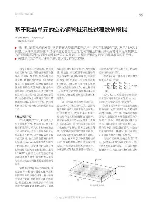
基于粘结单元的空心钢管桩沉桩过程数值模拟◎ 张琦 桂劲松 大连海洋大学通讯作者：桂劲松摘 要：随着技术的发展，钢管桩在大型海洋工程结构中的应用越来越广泛。

利用ABAQUS 有限元软件模拟实际施工过程中空心管桩与土壤之间的相互作用，并利用粘结单元来模拟土的开裂和挤压行为，通过将模拟结果与实际施工过程进行比较，验证了模拟模型的可行性。

关键词：粘结单元；锤击沉桩；贯入度；有限元模拟如今在建筑工程领域里，钢管桩的应用颇为广泛。

钢管桩基础具有强度高、自重轻、施工快、制作运输方便等优势。

随着科技的发展，钢结构防腐技术也愈发成熟，这使得钢管桩也越来越多的在大型海洋工程结构中得以应用。

数值模拟可以通过建立模型反映实际工程中复杂的应力应变关系、空心管桩与土体的相互作用以及模拟实际情况下的施工过程，是研究和解决工程中受力和变形问题的有力工具。

1.粘结单元介绍在ABAQUS软件中，粘结单元适用于建模粘合剂、粘结界面、垫片和岩石断裂等[1]。

单元的本构响应取决于具体的应用，并基于对变形和应力状态的某些假设，这些假设适用于每个应用区域。

在以往的数值模拟中采用Mohr-Coulomb弹塑性模型模拟土的屈服准则，本文通过粘结单元模拟钢管桩在进入土后排土效应，运用A BAQUS软件建立大直径空心管桩连续锤击贯入模型，将管桩贯入模拟与实际工程进行对比来验证模型的可行性。

粘结单元的设置方式有两种，分别是在Par t模块中创建实体单元和在网格划分过后自动设置。

第一种方法需要在Par t模块中先创建实体单元，然后通过材料的赋予实体单元粘结模型的属性来设置粘结单元。

通常可以通过材料的力学参数，如剪切模量、泊松比、弹性模量等来设置粘结单元的属性。

在实际应用中，这种方法需要将粘结单元与实体单元进行Tie绑定，以保证粘结单元和实体单元的连通性和协同工作。

在这种情况下，应该注意调整材料参数和Tie约束条件，以保证模拟结果的准确性和可靠性。

另一种方法是在网格划分过后，通过A BAQUS自带的工具，选择需要设置粘结单元的面进行自动设置。

关于Cohesive模型应用的一些小结学习粘聚力单元时从各种讨论中获益匪浅，现总结自己做过的一些练习模型，希望对大家有所帮助。

里面有很多是论坛中帖子里面的知识，在此对原作者一并谢过。

错误疏漏之处请大家多指正。

这里所有的粘聚力模型都是指Traction-separation-based modeling( The modeling of bonded interfaces in composite materials often involves situations where the intermediate glue material is very thin and for all practical purposes may be considered to be of zero thickness，帮助文献目录为32.5.1-2 )。

模型中参数仅作测试用，没有实际意义。

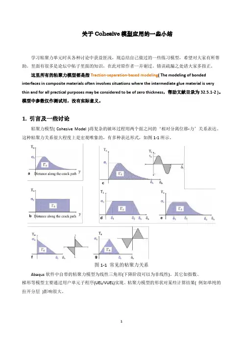
1.引言及一些讨论粘聚力模型( Cohesive Model )将复杂的破坏过程用两个面之间的‘相对分离位移-力’关系表达。

这种粘聚力关系很大程度上是宏观唯象的，有多种表达形式，如图1-1所示。

图1-1 常见的粘聚力关系Abaqus软件中自带的粘聚力模型为线性三角形(下降阶段可以为非线性)。

其它如指数、梯形等模型主要通过用户单元子程序(UEL/VUEL)实现。

粘聚力模型的形状对某些计算结果( 例如单纯的拉开分层)影响很大。

1.1 粘聚力单元及粘聚力接触粘聚力模型可以通过使用粘聚力单元( Cohesiev Elements )或者粘聚力接触( Cohesive Surfaces )来实现。

在模型和参数都一致的时候，两类方法得到的结果略有差别。

1.2粘聚力单元Abaqus中的粘聚力单元包括3D单元COH3D8，COH3D6；2D单元COH2D4；轴对称单元COHAX4；以及相应的孔压单元。

单元的厚度(分离)方向对于粘聚力单元，一个非常重要的方面是确定单元的厚度(分离)方向( Thickness direction、Stack direction )。

πH U max = Tsh(2πh / L)
H – 波高 h – 水深 T – 波周期
Umax – 泥沙的最大起动速度 当 Umax >Ut, 泥沙起动 一般砂质海岸的Mz为0.05-2.0mm. 当D>0.5mm时，
d0 ρUt = 0.46( ) ( ρ s − ρ ) gD D
2
1 4
环流和近岸流
Total load transport
Total load transport rate is the combination of bedload and suspended load transport Total load transport rate can be obtained by calculating bedload and suspended load transport rates separately and then adding up the two. Alternatively total sediment transport rate can be given by a single empirical formula.
上部
下部
“中立线"的位置取决于下列三个条件： 1.坡度较陡，对该剖面上各种粒径泥沙的中立线位置也 就愈靠近海岸和在深度较浅的地点。 2.当波浪较大时，它们的不对称性变形发展较快，在该 剖面上泥沙的中立线位处在岸外较远的较大水深处。 3.颗粒较大，其中立线应位处在离岸较远的地点。
英曼和巴格诺尔德取得了反映局部海滩坡度的关系式：
Relation of Engelund And Hansen (1972)
• It applies to flows and tidal currents • The friction coefficient CD must be determined by Englund (1966) alluvial friction method

Towards a Generalized Bounding Surface Model for Cohesive SoilsVictor N.Kaliakin 1and Andr´e s Nieto Leal 21Department of Civil &Environmental Engineering,University of Delaware,Newark,DE 19716;PH (302)831-2409;FAX (302)831-3640;email:kaliakin@ 2Department of Civil &Environmental Engineering,University of Delaware,Newark,DE 19716;PH (302)831-2409;FAX (302)831-3640;email:anieto@ ABSTRACTSince its inception over thirty years ago,the bounding surface model for cohe-sive soils has been progressively improved and expanded to a three-invariant,elasto-plastic formulation that accounts for the initial and stress induced anisotropy.More recently,a simplified version of the model served as the basis for a simplified form of the anisotropic model.In order to more accurately simulate the softening of natural clays,the associative flow rule used exclusively in all earlier versions of the model was recently extended to include a non-associative flow rule.In an effort to unify the afore-mentioned versions of the bounding surface model for cohesive soils,a generalized model framework has been developed.The present paper describes this framework.INTRODUCTIONBeginning with its inception in the 1980’s (Dafalias and Herrmann,1980,1982),the bounding surface model for cohesive soils has been progressively improved and expanded to a three-invariant,elastoplastic formulation (Dafalias,1986;Dafalias and Herrmann,1986).Notable milestones in the development of this model were the ability to account for initial and stress induced anisotropy (Anandarajah and Dafalias,1986)and then the ability to simulate the time-dependent response of isotropic cohesive soils within a combined and coupled elastoplastic-viscoplastic framework (Dafalias,1982;Kaliakin and Dafalias,1990a,b).Based on extensive experience,this version of the isotropic model was subsequently simplified (Kaliakin and Dafalias,1989).More recently,the simplified version of the model served as the basis for asimplified form of the anisotropic model (Ling et al.,2002).In order to more accurately simulate the softening of natural clays,the associative flow rule used exclusively in all earlier versions of the model was recently extended to include a non-associative flow rule (Jiang et al.,2012).In an effort to unify the aforementioned versions of the bounding surface modelfor cohesive soils,a generalized model framework has been developed.The present paper describes this framework.Following a general overview of the bounding surfaceD o w n l o a d e d f r o m a s c e l i b r a r y .o r g b y A n h u i U n i v e r s i t y o f T e c h n o l o g y o n 03/26/15. C o p y r i g h t A S CE .F o r p e r s o n a l u s e o n l y ; a l l r i g h t s r e s e r v e d .concept,the paper discusses the direct and joint invariants used in the model formula-tion,specific forms of the bounding surface,explicit expressions for isotropic and kine-matic hardening laws,and the shape hardening functions that constitute a novel aspect of bounding surface based models.A limited number of applications of the model to cohesive soils will also be presented.THE BOUNDING SURFACE IN STRESS SPACEThe bounding surface concept,originally introduced by Dafalias and Popov (1974)and independently by Krieg (1975),was motivated by the observation that any stress-strain curve for monotonic loading,or for monotonic loading followed by re-verse loading,eventually converges to certain well-defined “bounds”in the stress-strain space.These bounds cannot be crossed but may change position in the process of load-ing.For the development of constitutive models,the simplest way to describe the bounding state is by means of the concept of a bounding surface in stress space (Dafalias,1981).The bounding surface is the multiaxial generalization of the concept of “bounds”in the uniaxial stress-strain space.In this particular representation,appro-priate for soils,the bounding surface always encloses the origin and is origin-convex;i.e.,any radius emanating from the origin intersects the surface at only one point.The essence of the bounding surface concept is the hypothesis that plastic deformations can occur for stress states either within or on the bounding surface.Thus,unlike classi-cal yield surface plasticity,the plastic states are not restricted only to those lying on a surface.This fact has proven to be a great advantage of the bounding surface concept.If the material state is defined in terms of the effective stress σij (external vari-ables),and proper plastic internal variables q n ,then the bounding surface in effective stress space is defined analytically byF ¯σ ij ,q n =0(1)where a bar over stress quantities indicates an “image”point on the bounding surface.The actual stress point σij lies always within or on the surface.To each effective stressstate σ ij a unique “image”stress point ¯σij is assigned by a properly defined “mapping”rule that becomes the identity mapping if σij is on the surface.The Role of the Bounding SurfaceThe bounding surface is instrumental in defining the direction (or vector)of plastic loading-unloading L ij and the plastic modulus K p that enter into a typical elastoplasticity formulation.The expression for L ij at σij is defined as the gradient of F at the “image”point;viz.,L ij =∂F ∂¯σij(2)For any stress increment dσij causing plastic loading,a corresponding imageD o w n l o a d e d f r o m a s c e l i b r a r y .o r g b y A n h u i U n i v e r s i t y o f T e c h n o l o g y o n 03/26/15. C o p y r i g h t A S CE .F o r p e r s o n a l u s e o n l y ; a l l r i g h t s r e s e r v e d .stress increment ¯dσij occurs as a result of the hardening of the bounding surface by means of the internal variables q n .The following relations are thus required to com-plete the general bounding surface formulation:A scalar loading index that is definedin terms of equation (2),the stress increments dσij ,¯dσij ,the plastic modulus K p (as-sociated with σij )and a “bounding”plastic modulus ¯K p (associated with ¯σij )in thefollowing manner:L =1K p ∂F ∂¯σij dσij =1¯K p ∂F ∂¯σij d ¯σij (3)A bounding plastic modulus ¯Kp that is obtained from the consistency condition dF =0.Finally,a state-dependent relation between K p and ¯Kp that is established as a function of the Euclidean distance δbetween the current stress state and its “image”stress;viz.,K p =¯K p +ˆH (σij ,q n )δr −δ(4)Equation (4)embodies the meaning of the bounding surface concept.If δ<r and ˆH is not approaching infinity,the concept allows for plastic deformations to occur for points either within or on the surface at a progressive pace that depends upon δ.The closer to the surface is the actual stress point (σij ),the smaller is K p (itapproaches the corresponding ¯Kp ),and the greater is the plastic strain increment for a given stress increment.The σij may eventually reach (possibly asymptotically)the bounding surface in the course of plastic loading;it remains on the surface if loading continues,and detaches from the surface and moves inwards upon unloading.Thus,forstates within the bounding surface,the function ˆHalong with its associated parameters are intimately related to the material response,and as such,constitute important “new”elements of the present formulation with regard to ones based upon classical yield surface elastoplasticity.ELEMENTS OF A GENERALIZED BOUNDING SURFACE MODELA generalized bounding surface model for cohesive soils is described in termsof the following quantities:1)a properly defined strain decomposition,2)suitably cho-sen stress invariants,3)a set of internal variables,4)an appropriate definition of the elastic response,5)an explicit definition of the bounding surface,6)a failure crite-rion,7)suitable hardening rules,8)a shape hardening function,and 9)a set of model parameters,whose values are determined by matching numerical simulations with ex-perimental results.Details pertaining to each of the aforementioned quantities are dis-cussed below.Strain DecompositionThe general coupling that exists between plastic and viscoplastic processes re-quires the following additive strain decomposition:D o w n l o a d e d f r o m a s c e l i b r a r y .o r g b y A n h u i U n i v e r s i t y o f T e c h n o l o g y o n 03/26/15. C o p y r i g h t A S CE .F o r p e r s o n a l u s e o n l y ; a l l r i g h t s r e s e r v e d .˙εij =˙εe ij +˙εi ij =˙εe ij +˙εv ij +˙εp ij(5)where εij represents the total infinitesimal strain tensor and the superscripts e ,i ,vand p denote its elastic,inelastic,viscoplastic (delayed)and plastic (instantaneous)components,respectively.Choice of invariantsInvariance requirements under superposed rigid body rotation require that thebounding surface be a function of the direct and joint isotropic invariants of ¯σij and q n .The joint invariants characterize material anisotropy,and somewhat different forms of these invariants have been used in previous anisotropic versions of the model (Anan-darajah and Dafalias,1986;Ling et al.,2002;Jiang et al.,2012).These invariants are not required for isotropic versions of the model.Choice of internal variablesIn all of the previous versions of the bounding surface model for cohesive soils,the surface is assumed to undergo isotropic hardening along the hydrostatic (I 1)axis.The hardening is controlled by a single scalar internal variable that measures the in-elastic change in volumetric strain;viz.,˙εi kk =˙εv kk +˙εp kk(6)Definition of the elastic responseElastic isotropy has been assumed in all of the previous versions of the bound-ing surface model for cohesive soils.Furthermore,this isotropy is assumed to be inde-pendent of the rate of loading and to be unaltered by inelastic deformation.Explicit definition of the bounding surfaceEquation (1)gives the general analytical form of the bounding surface in stressinvariant space,which may assume many particular forms provided it satisfies certain requirements concerning the shape of the surface (Dafalias and Herrmann,1986).Two specific forms of the bounding surface have traditionally been associated with the mod-eling of cohesive soils.These are the “composite”form of the surface and the single ellipse.Motivated by the ideas of critical state soil mechanics,a specific form of thesurface consisting of two ellipses and a hyperbola with continuous tangents at their connecting points was developed (Dafalias and Herrmann,1980).Dafalias and Her-rmann (1986)present explicit expressions for F =0,which define each portion of thisD o w n l o a d e d f r o m a s c e l i b r a r y .o r g b y A n h u i U n i v e r s i t y o f T e c h n o l o g y o n 03/26/15. C o p y r i g h t A S CE .F o r p e r s o n a l u s e o n l y ; a l l r i g h t s r e s e r v e d .“composite”surface,along with derivatives of F with respect to the stress invariants.In an effort to simplify the formulation,a bounding surface consisting of a single ellipse has also been developed (Kaliakin and Dafalias,1989).This surface has been used in the more recent versions of the model (Kaliakin and Dafalias,1990a,b;Ling et al.,2002;Jiang et al.,2012).The failure criterionA critical state failure criterion has been assumed in all of the previous ver-sions of the bounding surface model for cohesive soils.For a specific value of the Lode angle θ,the failure surface is assumed to be straight and to coincide with the critical state line.In I 1−J space,the slope of the critical state line is denoted by N .The variation of N with θhas traditionally been described by a relation having the form N (θ)=g (θ,k )N c ,where k =N e /N c ,with N e =N (−π/6)and N c =N (π/6)be-ing the values of N associated with axisymmetric triaxial extension and compression,respectively.The dimensionless function g (θ,k )must take on the values g (−π/6,k )=k and g (π/6,k )=1.A simple form of this function,attributed to Gudehus (1973),and used by Dafalias and Herrmann (1986)in conjunction with bounding surface models for clays is g (θ,k )=2k/[1+k −(1−k )sin 3θ].Hardening rulesIn all of the previous versions of the bounding surface model for cohesivesoils,the surface is assumed to undergo isotropic hardening along the hydrostatic (I 1)axis.The hardening is controlled by a single scalar internal variable that mea-sures the inelastic change in volumetric strain given by equation (6).The simulation of material anisotropy requires that the surface also undergo rotational and possibly distortional hardening.The original rotational hardening rule proposed by Anandara-jah and Dafalias (1986)has been progressively simplified (Ling et al.,2002;Jiang et al.,2012).The distortional hardening rule originally proposed by Anandarajah and Dafalias (1986)has been removed from subsequent models (Ling et al.,2002;Jiang et al.,2012).Shape hardening functionThe hardening function ˆHdefines the shape of the response curves during in-elastic hardening (or softening)for points within the bounding surface.It relates theplastic modulus K p to its “bounding”value ¯Kp in the following general manner:K p =¯Kp +ˆH (σij ,q n )ˆf (δ)(7)This expression differentiates the bounding surface formulation from standard elasto-plasticity models.It is a generalization of equation (4);in that equation,ˆf(δ)=D o w n l o a d e d f r o m a s c e l i b r a r y .o r g b y A n h u i U n i v e r s i t y o f T e c h n o l o g y o n 03/26/15. C o p y r i g h t A S C E . F o r p e r s o n a l u s e o n l y ; a l l r i g h t s r e s e r v e d .δ/ r −δ .The plastic moduli K p and ¯Kp both have units of stress cubed (i.e.,F 3L −6).The “bounding”plastic modulus (¯Kp )is computed from the consistency condition.Since ˆf(δ)is dimensionless it follows that ˆH must also have units of stress cubed.Dif-ferent functional forms for ˆHhave been used in the past.For example,the bounding surface formulation for isotropic cohesive soils consisting of a single ellipse (Kaliakin and Dafalias,1989)used the following functional form of H :ˆH =(1+e in )λ−κP a 9(F,¯I 1)2+13(F,¯J )2h (θ)z 0.02+h o 1−z 0.02 f (8)In equation (8)e in denotes the initial void ratio.The critical state param-eters λand κare taken to denote the slopes of the isotropic consolidation andswell/recompression lines,respectively,in a plot of void ratio versus the natural log-arithm of I 1.The quantity P a denotes the atmospheric pressure,and z =J/J 1=JR/NI o is a dimensionless variable.The dimensionless quantity h (θa )defines the degree of hardening for points within the bounding surface,except those within the immediate vicinity of the I 1-axis where z →0.Of all the hardening quantities,h (θa )has the most fundamental and significant role.It is a function of the Lode angle θand varies in magnitude from a value of h c =h (π/6)(corresponding to a state of triaxial compression)to a value of h e =h (−π/6)(corresponding to a state triaxial extension).More precisely,this interpolation is given by h (θa )=g (θa ,k )h c =2µ/[1+µ−(1−µ)sin 3θa ]h c ,where µ=h e /h c .The quantity h o is the average of h c and h e .Finally,the function f is defined in the following manner:f =12a +sign (n p )(|n p |)1w where a and w are dimensionless model parameters.Finally,n p =3F,¯I 19(F,¯I 1)2+13(F,¯J )2is the component in the p -direction of the unit outward normal to the bounding surface in triaxial stress space.As such,it is a dimensionless quantity.Although the adoption of a single ellipse simplifies the explicit definition of the bounding surface,it requiresthe modification of previous functional forms of ˆH.More precisely,if a single ellipse is used instead of a hyperbola (which is closer to the critical state line),undesirably high levels of J will be attained at large overconsolidation ratios.To prevent this from occurring,the quantity f was added to the expression for H .SAMPLE APPLICATIONTo illustrate the capabilities of arguably the simplest form of the bounding sur-face model for cohesive soils,the isotropic model with associative flow (Kaliakin andD o w n l o a d e d f r o m a s c e l i b r a r y .o r g b y A n h u i U n i v e r s i t y o f T e c h n o l o g y o n 03/26/15. C o p y r i g h t A S CE .F o r p e r s o n a l u s e o n l y ; a l l r i g h t s r e s e r v e d .Dafalias,1989)was used to simulate the response of isotopically consolidated Lower Cromer Till (LCT)based on the work of Gens (1982).LCT is classified as a low-plasticity sandy silty-clay (liquid limit =25%and plasticity index =13%),with the main clay minerals being calcite and illite.The tests on LCT were all performed on samples consolidated from a slurry with an initial water content of 31%.Although the bounding surface model has traditionally been applied to rather soft clays with lager liquid limits and plasticity indices,the choice of LCT is motivated by its use in the verification of other clay models (Dafalias et al.,2006).Figure 1.Undrained stress paths for Lower Cromer Till.Values for the traditional critical state parameters were computed from the data of Gens (1982).In particular,λ=0.066,κ=0.0077,M c =1.18,M e =0.86,and ν=0.20.A value of 2.30for the parameter R defining the shape of the elliptical bounding surface was determined from the experimental undrained stress paths for normally consolidated samples in compression and extension.A value of 0.60for the projection center parameter C was determined by the shapes of the undrained stress paths for lightly overconsolidated samples.The rather “stiff”nature of these undrained stress required a value of 2.0for the elastic nucleus parameter s p .Finally,the following values were determined for the shape hardening parameters:h c =h e =1.0,a =6.0,and w =5.0.It is timely to note that the latter value has been used almost exclusively inD o w n l o a d e d f r o m a s c e l i b r a r y .o r g b y A n h u i U n i v e r s i t y o f T e c h n o l o g y o n 03/26/15. C o p y r i g h t A S CE .F o r p e r s o n a l u s e o n l y ; a l l r i g h t s r e s e r v e d .Figure 2.Deviator stress-axial strain response for Lower Cromer Till.previous simulations and can thus be taken as a model constant (as opposed to a model parameter).As evident from Figures 1and 2,even the simplest form of the bounding surface model for cohesive soils gives quite reasonable simulations for the undrained stress paths and stress-strain curves.CONCLUSIONA generalized definition of the bounding surface model for cohesive soils provides a convenient and elegant framework for unifying various versions of the model for both isotropically and anisotropically consolidated cohesive soils.This generalized defini-tion is described in terms of the following quantities:1)a properly defined strain de-composition,2)suitably chosen stress invariants,3)a set of internal variables,4)an appropriate definition of the elastic response,5)an explicit definition of the bounding surface,6)a failure criterion,7)suitable hardening rules,8)a shape hardening function,and 9)a set of model parameters,whose values are determined by matching numeri-cal simulations with experimental results.In the present paper a form of the model employing an associative flow rule,and formulated for isotropically consolidated soils has been shown to give quite good simulations for a low-plasticity sandy silty-clay.It is also timely to note that this simple form of the model has recently beenD o w n l o a d e d f r o m a s c e l i b r a r y .o r g b y A n h u i U n i v e r s i t y o f T e c h n o l o g y o n 03/26/15. C o p y r i g h t A S CE .F o r p e r s o n a l u s e o n l y ; a l l r i g h t s r e s e r v e d .used to successfully simulate a rather wide range of cohesive soils,subjected to both monotonic and cyclic loading histories.In particular,the response of Keuper Marl low plasticity silty clay (Yasuhara,et al.2003),Cloverdale clay (Zergoun,1991),a Kaoli-nite Clay (Li and Meissner,2002),and Bogota clay (Camacho and Reyes,2005)has also been successfully simulated.ACKNOWLEDGEMENTThe second authors graduate studies are supported by the Fulbright Colombia-COLCIENCIAS Scholarship.This support is gratefully acknowledged.REFERENCESAnandarajah,A.and Dafalias,Y .F.(1986).“Bounding Surface Plasticity III:Applica-tion to Anisotropic Cohesive Soils,”Journal of Engineering Mechanics,ASCE ,112(12),1292-1318.Camacho,J.and Reyes,O.(2005).“Aplication of modified cam-clay model to recon-stituted clays of the sabana of Bogota,”Ciencia e Ingeniera Neogranadina .Bogota,Colombia,20(1).Dafalias,Y .F.and Popov,E.P.(1974).“A Model of Nonlinearly Hardening Materialsfor Complex Loadings,”Acta Mechanica ,21(3),173-192.Dafalias,Y .F.(1981).“The Concept and Application of the Bounding Surface in Plas-ticity Theory,”IUTAM Symposium on Physical Non-Linearities in Structural Analysis ,Hult,J.and Lemaitre,J.eds.,Senlis,France,Springer-Verlag,Berlin-Heidelberg-New York,56-63.Dafalias,Y .F.(1982).“Bounding Surface Elastoplasticity -Viscoplasticity for Par-ticulate Cohesive Media,”Deformation and Failure of Granular Materi-als ,IUTAM Symposium on Deformation and Failure of Granular Materials,Delft,the Netherlands edited by P.A.Vermeer and H.J.Luger,Rotterdam:A.A.Balkema,97-107.Dafalias,Y .F.(1986).“Bounding Surface Plasticity.I:Mathematical Foundation andthe Concept of Hypoplasticity,”Journal of Engineering Mechanics,ASCE ,112(9),966-987.Dafalias,Y .F.and Herrmann,L.R.(1980).“A Bounding Surface Soil PlasticityModel,”Proceedings of the International Symposium on Soils Under Cyclic and Transient Loading ,edited by G.N.Pande and O.C.Zienkiewicz,Rotter-dam:A.A.Balkema,335-345.Dafalias,Y .F.and Herrmann,L.R.(1982).“A Generalized Bounding Surface Consti-tutive Model for Clays,”Application of Plasticity and Generalized Stress-Strain in Geotechnical Engineering ,edited by R.N.Yong and E.T.Selig,New York,ASCE,78-95.D o w n l o a d e d f r o m a s c e l i b r a r y .o r g b y A n h u i U n i v e r s i t y o f T e c h n o l o g y o n 03/26/15. C o p y r i g h t A S CE .F o r p e r s o n a l u s e o n l y ; a l l r i g h t s r e s e r v e d .iDafalias,Y .F.and Herrmann,L.R.(1986).“Bounding Surface Plasticity II:Appli-cation to Isotropic Cohesive Soils,”Journal of Engineering Mechanics,ASCE ,112(12),1263-1291.Dafalias,Y .F.,Manzari,M.T.and Papadimitriou,A.G.(2006).“SANICLAY:sim-ple anisotropic clay plasticity model,”International Journal for Numerical and Analytical Methods in Geomechanics ,30(12),1231-1257.Gens A.(1982).“Stressstrain and strength of a low plasticity clay,”Ph.D.Thesis,Im-perial College,London University,856.Gudehus,G.(1973).“Elastoplastische Stoffgleichungen f¨u r trockenen Sand,”Ingenieur-Archiv ,42(3),151-169.Jiang,J.,Ling,H.I.and Kaliakin,V .N.(2012).“An Associative and Non-AssociativeAnisotropic Bounding Surface Model for Clay,”Journal of Applied Mechanics,ASME (Jim Rice Special Edition),79(3),031010-1-131010-10.Kaliakin,V .N.and Dafalias,Y .F.(1989).“Simplifications to the Bounding SurfaceModel for Cohesive Soils,”International Journal for Numerical and Analytical Methods in Geomechanics ,13(1),91-100.Kaliakin,V .N.and Dafalias,Y .F.(1990a).“Theoretical Aspects of the Elastoplastic-Viscoplastic Bounding Surface Model for Cohesive Soils,”Soils and Founda-tions ,30(3),11-24.Kaliakin,V .N.and Dafalias,Y . F.(1990b).“Verification of the Elastoplastic-Viscoplastic Bounding Surface Model for Cohesive Soils,”Soils and Founda-tions ,30(3),25-36.Krieg,R.D.(1975).“A Practical Two Surface Plasticity Theory,”Journal of AppliedMechanics,ASME ,42(3)641-646.Li,T.and Meissner,H.(2002).“Two-surface plasticity model for cyclic undrained be-havior of clays,”Journal of Geotechnical and Geoenvironmental Engineering ,ASCE,128(7),613-626.Ling,H.I.,Yue,D.,Kaliakin,V .N.and Themelis,N.J.(2002).“An Anisotropic Elasto-Plastic Bounding Surface Model for Cohesive Soils,”Journal of Engineering Mechanics,ASCE ,128(7),748-758.Yasuhara,K.,Murakami,S.,Song,B.W.,Yokokawa,S.and Hyde,A.F.L.(2003).“Postcyclic Degradation of Strength and Stiffness for Low Plasticity Silt,”Jour-nal of Geotechnical and Geoenvironmental Engineering ,ASCE,129(8),756-769.Zergoun,M.(1991).Effective stress response of clay to undrained cyclic loading,PhDthesis,University of British Columbia.D o w n l o a d e d f r o m a s c e l i b r a r y .o r g b y A n h u i U n i v e r s i t y o f T e c h n o l o g y o n 03/26/15. C o p y r i g h t A S CE .F o r p e r s o n a l u s e o n l y ; a l l r i g h t s r e s e r v e d .。

MIKE 21 & MIKE 3非结构网格水流模型泥模块概述MIKE 21 & MIKE 3非结构网格水流模型–泥模块本文档描述了DHI公司最新的二维、三维非结构网格水流模型（FM）中的泥模块（MT）。

MT模块中的泥输移模型可以模拟粘性泥沙在海洋、微咸水、淡水中的侵蚀、输移、沉降和淤积过程。

该模块还可模拟细颗粒非粘性泥沙。

实例：丹麦Øresund疏浚泥沙的扩散MT模块是MIKE 21和MIKE 3非结构水动力模型中的附加模块。

对于底部固结层，需建立水动力结果与输移结果的连接（平流扩散模型）。

水动力基础由MIKE 21或MIKE 3非结构水流模型的水动力模块提供。

通过引入波谱（Spectral Wave）模块，（MIKE 21 FM SW）可以计算波浪对侵蚀/淤积的影响。

对于FM系列，可以将各模块进行动态链接并运行。

如果研究区域的地形变化与水深的变化幅度是同一数量级的，则有必要考虑地形对水动力的影响。

海床更新与水流之间的水动力反馈机制的选择可能在浅水区比较重要，例如，需考虑该区域的长期作用效果。

此外，在浅水区规划大量的维护疏浚，类似的，疏浚物的处理点，在这些区域可选择水动力的反馈机制。

实例：瑞典MalmÖ附近河流中泥沙羽状锋应用领域MT模块应用于粘性泥沙的侵蚀、扩散和淤积。

细颗粒泥沙作用于多方面。

在悬浮物方面，细颗粒泥沙可能会在一定时间内遮蔽部分水域，影响光照。

光照是底栖动植物生存的关键条件。

细颗粒泥沙可能会淤积于一些非理想区域，例如在港口的入口。

此外，污染物（如重金属、TBT）易吸附于粘性泥沙。

如果被污染的泥沙淤积于生态学上的敏感区域，将会对当地的动植物及水质造成重大影响。

实例：在近岸水域的再悬浮泥沙(Caravelas, Brazil)。

如对于疏浚问题，需要将背景沙场和外源泥沙区分开时，需考虑泥沙再悬浮问题。

估算淤积率是MT模块的一个常见应用领域，也是一个重要方面，例如设计航道的新入口或者加深航道，使更大的船只能进入港口。

Christopher D.CeraIlya Braude Geometric and Intelligent Computing Laboratory,Department of Computer Science,Drexel University,Philadelphia,PA19104Taeseong KimMobile Multimedia Laboratory, LG Electronics Institute of Technology,Seoul,137-724,KoreaJungHyun Han Department of Computer Science andEngineering,Korea University,Seoul,136-701,KoreaWilliam C.Regli Geometric and Intelligent Computing Laboratory,Department of Computer Science,Drexel University,Philadelphia,PA19104Hierarchical Role-Based Viewing for Multilevel Information Security in Collaborative CAD Information security and assurance are new frontiers for collaborative design.In this context,information assurance(IA)refers to methodologies to protect engineering infor-mation by ensuring its availability,confidentiality,integrity,nonrepudiation,authentica-tion,access control,etc.In collaborative design,IA techniques are needed to protect intellectual property,establish security privileges and create“need to know”protections on critical features.This paper provides a framework for information assurance within collaborative design based on a technique we call Role-Based Viewing.We extend upon prior work to present Hierarchical Role-Based Viewing as a moreflexible and practical approach since role hierarchies naturally reflect an organization’s lines of authority and responsibility.We establish a direct correspondence between multilevel security and mul-tiresolution surfaces where a hierarchy is represented as a weighted directed acyclic graph.The permission discovery process is formalized as a graph reachability problem and the path-cost can be used as input to a multiresolution function.By incorporating security with collaborative design,the costs and risks incurred by multiorganizational collaboration can be reduced.The authors believe that this work is thefirst of its kind to unite multilevel security and information clouded with geometric data,including multi-resolution surfaces,in thefields of computer-aided design and collaborative engineering.͓DOI:10.1115/1.2161226͔1IntroductionInformation assurance͑IA͒refers to methodologies to protect and defend information and information systems by ensuring their availability,integrity,authentication,confidentiality,and nonrepu-diation.In collaborative design,IA is mission-critical.Suppose a team of designers is working collaboratively on a3D assembly model.Each designer has a different set of security privileges and no one in the team has the“need to know”the details of the entire design.In collaboration,designers must interface with others’components/assemblies,but do so in a way that provides each designer with only the level of information he or she is permitted to have about each of the components.For example,one may need to know the exact shape of some portion of the part͑includ-ing mating features͒being created by another designer,but not the specifics of any other aspects of the part.Such a need can also be found when manufacturers outsource designing a subsystem: manufacturers may want to hide some critical information of the entire system from suppliers.The authors believe that a geometric approach to IA represents a new problem that needs to be addressed in the development of collaborative CAD systems.The approach we develop has many uses visible across several significant scenarios we envision for applying this work:Protection of sensitive design information:As noted above, designers may have“need to know”rights based on legal,intel-lectual property,or national security requirements. Collaborative supply chains:Engineering enterprises out-source a considerable amount of design and manufacturing activ-ity.In many situations,the organization needs to provide vital design data to one partner while protecting the intellectual prop-erty of another partner.Multidisciplinary design:For designers of different disci-plines working on common design models,designers suffer from cognitive distraction when they must interact with unnecessary design details that they do not understand and cannot change.For example,an aircraft wheel well͓1͔is a complex and confusing place in which electronics,mechanical,and hydraulics engineers all must interact in close quarters with vast amounts of detailed design data.These interactions could be made more efficient if the design space could be simplified to show each engineer only the details they need to see.This paper develops a new technique for Role-Based Viewing ͓2͔in a collaborative3D assembly design environment,where multiple users work simultaneously over the network,and pre-sents a combination of multiresolution geometry and multilevel information security models.Among various issues in IA,access-control is critical for the purpose.We demonstrate the specifica-tion of access privileges to geometric partitions in3D assembly models defined based on the Bell-La Padula model.Aside from digital3D watermarking,research on how to provide IA to dis-tributed engineering teams,working in collaborative graphical en-vironments,remains a novel and relatively unexplored area.We achieve these functional capabilities within a system designed for secure,real-time collaborative viewing of3D models by multiple users working synchronously over the internet on standard graph-ics workstations.The contributions of this work,developed in͓2͔, include:Providing a geometric approach to Information Assurance:Our work augments currently practiced access-control techniques in collaborative CAD and PDM systems.Although most of these systems offer access-control facilities,they are often limited to prohibiting access to models and documents and not partitions of geometry.Developing alternatives to the problem of“all-or-nothing”per-Contributed by the Engineering Simulation and Visualization of ASME for pub-lication in the J OURNAL OF C OMPUTING AND I NFORMATION S CIENCE IN E NGINEERING.Manuscript received January26,2004;final manuscript received March24,2005.Assoc.Editor:N.Patrikalakis.2/Vol.6,MARCH2006Copyright©2006by ASME Transactions of the ASMEmissions:The standard method for handling a lack of appropriate permissions is suppression of the sensitive features.This work attempts to highlight some alternatives other than the traditional solution.In our revised method,we show how geometric partitions are used to create multiple level-of-detail͑LOD͒meshes across parts and subassemblies to provide a Role-based View suitable for a user with a given level of security clearance.The specific contri-butions of this paper include:Introducing role hierarchies:We revisit the problem of role-based viewing in an updated context using role hierarchies.A hierarchy is represented as a weighted directed acyclic graph ͑DAG͒,and the permission discovery process is formalized as agraph reachability problem.Outlining the relation between multilevel security͑MLS͒hier-archies and multiresolution surfaces:In͓2͔we introduced a mul-tiresolution envelope to degrade surface features for a sensitive part or subassembly where details need to be withheld.We incor-porate this approach into role-hierarchies where the path-cost is used as input to a multiresolution function.The authors believe that this work represents a unique application of multiresolution surfaces to multilevel information security in computer-aided de-sign and collaborative engineering.This paper is organized as follows:Sec.2describes related work from information assurance,collaborative design,and com-puter graphics communities.Section3first reviews the specifica-tion of security features in thefields of solid modeling and engi-neering as outlined in Ref.͓2͔,then presents Hierarchical Role-Based Viewing.Section4explains the details of our multiresolution security model and outlines its relation to the Role Hierarchy.Section5describes the implementation of our proto-type system,and demonstrates a sample scenario using our stly,Sec.7summarizes our results,presents our con-clusions,and outlines goals for future research.2Related WorkThe contributions presented in this paper are related to infor-mation assurance,collaborative design,and multiresolution sur-face generation.2.1Information Assurance and Security.Current research on information assurance incorporates a broad range of areas fo-cused on protecting information and information systems by en-suring their availability,integrity,confidentiality,nonrepudiation, authentication,and controlling modes of rmation as-surance research,in the context of the CAD domain,has been partially addressed by the computer graphics community through the development of3D digital watermarking͓3͔.Digital Water-marking is used to ensure that the integrity of a model has been maintained,as well as provide a foundation for proof of copyright infringement.Other areas of research have been in authentication and access-control.We will introduce past and present research on access control methodologies and outline the differences between the varying policies.There is a clear distinction between authentication and access control services.Authentication services are used to correctly de-termine the identity of a user.Access control is the process of limiting access to resources of a system only to authorized users, programs,processes,or other systems.Authentication is closely coupled with access control,where access control assumes that users of an information system have properly been identified by the system.If the authentication mechanism of a system has been compromised,then the access control mechanism that follows will certainly be compromised.The primary focus of our work is to articulate an access control policy,specifically for the geometry of a solid model,assuming a robust authentication mechanism has already been established.Access-control literature describes high-level policies on how accesses are controlled,as well as low-level mechanisms that implement those policies.The common access control policies found in literature are Dis-cretionary,Lattice-Based,and Mandatory Access Control͑DAC,LBAC,and MAC,respectively͒.DAC was formally introducedby Lampson͓4͔,where essentially the owner of an object hasdiscretion over what users were authorized to access that object.Access broadly refers to a particular mode of operation such asread or write.The owner is typically designated as the creator ofan object,hence it is an actual user of the system.This is differentfrom LBAC and MAC,which we will refer to collectively asMAC͓5͔,where individual users have no discretion over objectaccess.MAC͓6͔is primarily concerned with theflow of informa-tion,thereby enforcing restrictions on the direction of communi-cation channels.For further discussion on access control policies,we refer interested readers to a survey by Sandhu͓7͔.Role-Based Access Control͑Group policies found in currentoperating systems could be viewed as an instance of hierarchicalRBAC͒.RBAC is an emerging area of study,and is actively pur-sued as an augmentation of traditional DAC and MAC.RBAC isa type of Multi-Level Security͑MLS͒framework,which is anactively pursued area in the database community͓8,9͔.In RBAC,individual users are assigned to roles,and the access permissionsof an object are also assigned to roles.Therefore the permissionsassigned to a role are acquired by the members associated with it.This additional layer reduces the management of permissions andsupports the concepts of least privilege,separation of duties,anddata abstraction.RBAC,and its associated components,are aninstrument for expressing a policy,and not a policy by itself.Forrole-based viewing,we use a MAC policy embodied within an RBAC framework.2.2Collaborative Design.There is a vast body of work on concurrent engineering and distributed collaborative design.Visu-alization and multiuser protocols were the primary focus of manyearly systems,and generally fell under the terms Distributedand/or Collaborative Virtual Environments͓10–17͔.Thereafter,lightweight design͓18–21͔and assembly modeling systems͓22͔for distributed CAD began to emerge.With the demand for distributed CAD and more edit-drivenmodeling mechanisms,several research systems and commercialproducts have reached fruition.Current work in distributed col-laborative design,with respect to geometry,can be“loosely”grouped into two categories:visualization and annotation of CADmodels;co-design and manipulation of CAD geometry.The cur-rent demonstration of our work is primarily targeted at the formercategory.This is complementary to facet-based editing techniques ͓23͔,however editing multiresolution geometry hierarchies can be extended to feature,assembly,and native-geometry editing facili-ties.This assumes a system with policies that permit editing on alow resolution model,where the user in question does not havepermissions to view the full resolution model.Polyinsantiationissues are beyond the scope of this paper,although most theoret-ical issues have been developed with regard to databases͓8,9͔.The generation of facets is inevitable in the visualization pro-cess,and most distributed CAD systems deal with this problem invery diverse ways.System designers must resolve varying trade-offs in the areas of visualization,editing mechanisms,bandwidthutilization,and accuracy.Some systems have targeted view-dependent techniques as an attempt to reduce aggregate band-width and computation͓24–27͔.Current literature now providesnumerous mechanisms and interfaces from which to edit CADmodels:features͓28,29͔;assemblies͓30,31͔;native surfaces͑e.g.,b-rep͓͒32,33͔;and facet-based techniques͓23͔.The heterogeneity of existing systems and interchange formats further complicates the domain.Reference͓28͔contains an extensive overview of current distributed CAD systems from the perspective of architec-ture and data exchange.2.3Multiresolution Techniques.Polygon meshes lend them-selves to fast rendering algorithms,which are hardware-accelerated in most platforms.Most CAD models are representedJournal of Computing and Information Science in Engineering MARCH2006,Vol.6/3as a set of trimmed parametric surfaces,so tessellation to a desired resolution is performed ͓34,35͔.Many applications,including CAD,require highly detailed models to maintain a convincing level of realism.It is often necessary to provide LOD techniques in order to deliver real-time computer graphics and animations.Therefore,mesh simplification is adopted for efficient rendering and transmission.The most common use of mesh simplification is to generate multiresolution models or various levels of detail ͑LOD ͒.For example,closer objects are rendered with a higher LOD,and distant objects with a lower LOD.Thanks to LOD management,many applications such as CAD visualization can accelerate rendering and increase interactivity.A survey on mesh simplification can be found in Ref.͓36͔.The most popular polygon-reduction technique is an edge col-lapse or simply ecol ͑more generally,vertex merging or vertex pair contraction ͒where two vertices are collapsed into a single one.The issues in ecol include which vertices to merge in what order,where to place the resulting vertex,etc.Vertex split or sim-ply vsplit is the inverse operation of ecol .These operations are illustrated in Fig.1͑a ͒and a sequence of operations is illustrated on a sample model given in Fig.1͑b ͒.Hoppe proposed the progressive mesh ͑PM ͓͒38͔,which con-sists of a coarse base mesh ͑created by a sequence of ecol opera-tions ͒and a sequence of vsplit operations.Applying a subset of vsplit operations to the base mesh creates an intermediate simpli-fication.The vsplit and ecol operations are known to be fast enough to apply at runtime,therefore supporting dynamic simpli-fication.3Role-Based ViewingIn the context of 3D design,a model M is a description of an artifact,usually an individual part or assembly,in the form of a solid model.A true collaborative engineering environment enables multiple engineers to simultaneously work with M .The engineers ͑designers,process engineers,etc ͒correspond to a set of actors A =͕a 0,a 1,...,a n ͖each of which has associated with it a set of roles .Roles,R =͕r 0,r 1,...,r m ͖,define access and interaction rights for the actors.For example,actor a 3might have associated with it roles,r 20,r 23,and r 75—this entitles a 3to view ͑and per-haps change ͒portions of M associated with these roles.Portions of M not associated with these roles,however,might be “off lim-its”to actor a 3.This section will build on the results of Ref.͓2͔,where Role-based Viewing was developed in the context of dis-tributed collaborative CAD,by introducing role hierarchies and their relation to multiresolution surfaces.We formulate the problem of role-based viewing in the follow-ing subsections by developing:͑a ͒Actor-role framework:a general RBAC framework for describing actors and roles within a collaborative-distributed design environment.This framework uses a hierarchical graph to capture role-role relationships and create a relation between actors and roles.͑b ͒Model-role framework:an associative mapping from roles to topological regions on models.These regionscapture the security features ,F ,of a 3D model—relating how a point,patch,part,or assembly can be viewed by actors with given roles.͑c ͒Hierarchical role-based viewing:an algorithm to generate a role-based view given an actor a ,his/her set of roles,the role hierarchy ͑RH ͒,a model M ,and its set of secu-rity features.A role-based view is a tailored 3D model which is customized for actor a based on the roles defin-ing a ’s access permissions on the model.In this way,the role-based view model does not compromise sensitive model information which a is not allowed to see ͑or see in detail ͒.This is accomplished using a mesh simplifica-tion technique to generate the role-based view .3.1Actor-Role Security Framework.Our security frame-work is based on an adaptation of role-based access control,as developed in the information assurance and security literature ͓39͔,to the collaborative design problem.We focus on the relation between actors,their roles and the solid model geometry.This is in contrast to other work on access control in collaborative CAD which has focused mainly on database synchronization/transaction issues ͓40͔.Representing actors and roles:We define a hierarchical RBAC framework where:͑1͒Entities include a set of actors,A =͕a 0,a 1,...,a n ͖and a setof roles r =͕r 0,r 1,...,r m ͖;͑2͒Actor-role assignment,AR,is a relation ͑possibly many-to-many ͒of actors to roles:AR ʕA ϫR ;͑3͒Role hierarchy,RH,captures the relationships among theroles.For example,the permissions entailed by role r 75might be a superset of those entailed by.Hence,the role hierarchy is a weighted ,directed acyclic graph ͑DAG ͒,RH=͑R ,H ͒,where H ʚR ϫR is the hierarchical set of re-lationships ͑edges ͒among the roles in R .This creates a partial order on R ,hence ͑in the example above ͒if ͗r 23,r 75͘෈H then r 23՞r 75.The weight of each edge in H is given by the real-valued function w :H →͓0,1͔.An example of this RBAC framework is given in Fig.2.For the remainder of this paper,we focus on read/viewing permissions granted by a given set of roles.Rather than “all or nothing”read permissions,our objective is to assign a “degree of visibility”to features of a model based on an actor’s ing this formu-lation,we show how one can implement a Bell-La Padula-based ͓6͔security model for collaborative viewing of CADdata.Fig.1Illustration of multiresolution techniques.…a …Edge collapse …ecol …and vertex split …vs-plit …operations.v t …top …and v b …bottom …collapse into v m …middle ….The inverse operation in-volves splitting v m back into v t and v b .…b …Sequence of operations on the “socket”model †37‡.Fig.2Example actor-role …AR …and role hierarchy …RH …assignments4/Vol.6,MARCH 2006Transactions of the ASMEExample :Using the simple actor-role assignment matrix and role hierarchy from Fig.2,we can compute the degree of visibility to each actor for a model assigned to a specific role.To implement the Bell-La Padula ͓6͔model,we need to compute visibility in such a way as to guarantee that the role ͑e.g.,security clearance ͒of someone receiving a piece of information must be at least as high as the role assigned to the information itself.In this way,a CAD model classified as “Secret”can only be viewed by those with a “Top-Secret”or “Secret”classification,but not viewed by someone with only a “Confidential”level of access.Figure 3il-lustrates this example.3.2Model-Role Security Framework.Let M be a solid model of an artifact ͑part,assembly,etc.͒and let b ͑M ͒represent the boundary of M .In this context,the Model-Role Assignment ,MR,is a relation ͑possibly many-to-many ͒assigning roles to points on the surface of the model:MR ʕb ͑M ͒ϫR ,where each point on b ͑M ͒has at least one role ͑i.e.,"p ෈b ͑M ͒,$r ෈R such that ͗p ,r ͘෈MR ͒.In this way,each point on the surface of the solid model M has associated with it some set of access rights dependent on the roles associated with it.In practice,it is impractical to assign roles point-by-point to the b ͑M ͒.Hence,we define a set of security features ,f =͕f 0,f 1,...,f k ͖,where each f i is a topologically connected patch on b ͑M ͒and ഫF =b ͑M ͒;and each f i has a common set of role assignments.Therefore,the Model-Role assignment can be sim-plified to be the relation associating security features with access roles:MR ʕF ϫR .Example :Let M be a solid model;let,F =͕f 1͖,where f 1=b ͑M ͒͑i.e.,the entire boundary is one security feature ͒.If MR =͕͗f 1,r 0͖͑͘where r 0is from the previous example in Fig.3͒,then we can see the resultant model for r 0depicted in Fig.4.3.3Hierarchical Role-Based Viewing.The issue now is that,for a given actor a ,what portions of the model M that he/she can see will depend on their associated roles and the security features of the model.Depending on their permissions,a new model,M Ј,must be generated from M such that the security features are not shown or obfuscated based on the actor’s roles.If their roles give them permission to see certain features ͑i.e.,mating features ͒,then the resulting model includes the features with the same fidelity ͓41͔as in M ;if not,the features must be obfuscated in such a way as to hide from a what a does not have the right to see.Hence,the role-based view generation problem can be stated:Problem :Given a set of roles and their relationships ͑R and RH ͒;a solid model and its security features ͑M ,F ,and MR ͒;and an actor ͑a and AR ͒,determine the appropriate view M Јof modelM for actor a .We propose a solution based on the use of multiresolution meshes,as follows:͑1͒Convert solid model M to a high-fidelity mesh representa-tion;͑2͒Based on F ,determine which facets belong to each securityfeature,f ;͑3͒For each security feature f ,do:͑a ͒If the intersection of actor a ’s roles and f ’s roles isnonempty,then add the facets associated with f to M Ј;͑b ͒If actor a ’s roles do not intersect the roles of f ,deter-mine ͑using RH ͒how much of f they are allowed to see and create a set of modified facets to represent f for inclusion in M Ј.͑4͒Clean up the resulting M Јso that boundaries of the f i ’s aretopologically valid.͑5͒Return M Ј.There are three research problems we address:͑1͒How does the role-hierarchy RH relate to the degree ofvisibility?We show how the weighted DAG that comprises RH can be used to implement a number of useful security policies by making the model quality a function of the path-cost among roles in RH.͑2͒How to modify the facets for each f i based on RH?Our approach is to use a security policy ͑based on Bell-La Padula ͒associated with the role hierarchy RH to determine how to modify the model.In some cases,policy will dictate degradation of the model fidelity;in other cases,the security features may be completely deleted or replaced with a simple convex hull or bounding box as in Ref.͓2͔.To accomplish this,we employ multiresolution meshes:model fidelity will be preserved to the degree the actor’s rights allow it.The result is a mesh appropriate for viewing by the actor a .͑3͒How to ensure that the resulting regions form a topologi-cally valid model?Deforming the model feature by feature may result in topological regions of facets in M Јthat are misaligned or aesthetically unpleasing.Cracks and occlusion can be avoided by preserving the boundary edges during simplification.Example :This example shows a model M whose surface is described by one security feature f 0.Given the role-hierarchy from Fig.3,and four actors,a 0,a 1,a 2,and a 3with their AR shown in Fig.2.Figure 5shows the four different views of model M they each see.Given the AR,RH,and MR assignments,we can derive the direct actor ϫfeature mappings.Figure 6gives the di-rect mappings specified implicitly by the AR,RH,and MR given in Figs.2͑a ͒,2͑b ͒,and 5respectively.The two MR assignments that are not shown are f 1෈r 1and f 2෈r 2.It is important to note that,similar to inheritance found in most object-oriented program-ming languages,a 0cannot see f 1or f 2even though it is the base role for subroles r 1,r 2,and r 3.Hence an inheritance relation al-lows a child to inherit the permissions of the parent,but nothing is implied in the other direction.4Technical ApproachWe combine techniques from solid modeling and computer graphics to provide a secure collaborative environment which sup-ports real-time design.In this section we describe how to modify and configure Hierarchical RBAC to support our multiresolution security model.We describe the problems,algorithms employed,and finalconsiderations.Fig.3An example weighted role hierarchy with associatedlabelsFig.4An example part with one security feature where b …M …is assigned to r 0Journal of Computing and Information Science in EngineeringMARCH 2006,Vol.6/54.1Hierarchical RBAC Policy.Since RBAC is a means of articulating policy rather than a policy by itself,an actual policy is necessary.We wish to adopt a policy similar to the classical MAC model ͓6͔.This is defined in terms of the following axioms using ␭to return the security level of either an actor or a feature:͑1͒Simple security property:Actor a can read feature f iff␭͑a ͒ജ␭͑f ͒.This is also known as the read-down property.͑2͒Liberal ء-property:Actor a can write feature f iff ␭͑a ͒ഛ␭͑f ͒.This is also known as the write-up property.There are many variations of the ء-property,but we will focus on the simple security property which essentially states that the clearance of a person receiving a piece of information must be at least as high as the classification of the object.Details on a formal construction of MAC in RBAC have been presented by Osborn ͓5͔.Hierarchical RBAC is a natural means for structuring roles thatreflect an organization’s lines of authority and responsibility ͓39͔.The main distinction between our approach and the generic RBAC frameworks found in literature,is that we also allow per-missions to be modified through the role hierarchy .Typically per-missions ͑i.e.,an object and a permissible operation ͒are associ-ated with every combination of object ϫrole .Since our read permissions are specified by a degree of visibility value,an inher-itance relation can further refine this value.An inheritance relation is a binary relation ͑parent ,child ͒,where the child inherits per-missions from the parent based upon a multiplicative weight w .For instance:w =1.0preserves the parents permissions exactly,while w =0.5will reduce the degree of visibility by half for all inherited objects.By transitivity,this weighted factor applies to all inherited objects specified in the role hierarchy.Intuitively,it might appear that we are breaking the simple se-curity property by allowing some actors to view objects that they normally would not be able to see.This is not the case,and in-stead should be viewed as transforming one object into a new object that is permissible.Hence,our model still adheres to the simple security property.Given an actor ͑a ͒and a feature ͑f ͒,the test to determine if a has permissions on f is equivalent to computing graph reachability among all possible pairs of roles assigned to both a and f .We will use R a to denote the set of roles assigned to a ,and R f for the set of roles assigned to f .If any role in R a is reachable from any other role in R f ͑i.e.,there exists a path ͒,then the product of all weights along the path yields the degree of visibility for that path.We will use a reachability function to return the set of all roles reachable from a given role.Several paths are possible,hence the resultant degree of visibility for a will be chosen as the maximum.We denote the function that returns the maximum degree of visibility for a on f as ␣͑a ,f ͒.The result of this function can be computed once,stored,and reused until an existing role assignment ͑AR or MR ͒is modified.The degree of visibility is then used as a param-eter to another function which degrades the fidelity of a feature depending on an actors permissions.4.2Generation of Multilevel Security Models.For part/component/assemblies with regions that need to be secured,mul-tiresolution techniques are employed to provide various levels of detail.Although the original ͑highest ͒resolution version of a model might be a breach for some actors,lower resolution LODs will be sufficiently secure to transmit to those actors.In addition to purely geometric multiresolution techniques,Shyamsundar and Gadh have developed a framework for representing different lev-els of detail for geometric feature data ͓31,42͔.Our security model could be used in conjunction with this feature LOD representa-tion,but an automatic simplification algorithm needs to be developed.Mesh simplification techniques include either vertex decima-tion,vertex clustering,or edge contraction.Choosing a specific simplification technique among the breadth of candidates is appli-cation dependent.To address the demands of an interactive col-laborative design environment,we outline several issues which are critical for simplification:͑1͒Speed :As the number of component/assemblies in a sessionincreases,the simplification becomes the bottleneck.We need an algorithm capable of drastic simplification in the least amount of time.͑2͒Continuous :A continuous spectrum of detail is necessaryso an appropriate model can be selected at runtime.We do not wish to store all possible LODs within the model re-pository due to space constraints,but parameters of the simplification hierarchy can be precomputed and stored.͑3͒Boundary preserving :The boundary of objects should bepreserved in order to distinguish objects from one another.Inadvertent occlusion and cracks may result if we relieve this constraint.͑4͒View-independence :The viewer receives 3D modelinfor-Fig.5An example part with one security feature …f 0…consist-ing of b …M …assigned to r 0,a set of actors assigned to roles,and their corresponding set of securemodelsFig.6The direct permission mappings derived from the AR,RH,and MR relations given in Figs.2…a …,2…b …,and 5,respectively6/Vol.6,MARCH 2006Transactions of the ASME。

3471
hesive laws which was pioneered by Dugdale (Dugdale 1960) and Barenblatt (Barenblatt 1962), has been successfully used in a Finite Element setting by several researchers (Xu and Needleman 1994, Ortiz and Pandolfi 1999). In summary, according to this model, fracture is a gradual phenomenon in which separation takes place across an extended crack ’tip’ or cohesive zone and is resisted by cohesive tractions. This theory of fracture allows the incorporation into the analysis of well-established fracture parameters such as the spall strength (i.e. the peak cohesive traction) and the fracture energy of the material which is represented by the area under the cohesive law. The present study focuses on the fatigue life calculations using a cohesive zone model (CZM). The details of the model and its finite element implementation are discussed in the following section. Even though it provides an accurate tool, the computational cost required to perform a full analysis over hundreds of thousands or millions of cycles would be tremendous. A time acceleration procedure is proposed to alleviate this problem in section 3. Undeniably, uncertainties play a pivotal role in the prediction of fatigue life. On one hand they explain the statistical scatter observed in experimental data and on the other hand their incorporation in the analysis offers a rational framework for quantifying the reliability and serviceability of those components. Applications in aerospace components are discussed in the final section where a probabilistic model for the incorporation of uncertainties in the material fracture properties is also presented. 2 COHESIVE ELEMENT MODEL 2.1 Triangular Cohesive Zone Model In the present study, a cohesive zone element model with a Rankine type activation criterion is advocated because it combines sufficent accuracy in the modeling of crack formation and computational efficiency which is an essential requirement when carrying out fatigue life calculations. Cohesive zone models were pioneered by Dugdale (Dugdale 1960) and Barenblatt (Barenblatt 1962) in order to overcome the contradictions of infinite stresses at the crack tip that classical linear or nonlinear elasticity predicted. Instead they assumed the existence of a zero-thickness process zone which is precursor to the formation of a new crack. The faces of the process zone are gradually separating while finite cohesive tractions develop which tend to resist the formation of the new surface. They eventually reduce to zero upon attainment of a critical separation. The advent of computers and the explosive progress in finite element technologies gave rise to

中英文参考文献参考文献[1] 许永兵, 朱方正. 城市过江通道的建设和发展分析[J]. 公路与汽运, 2010(2):39-41.[2] 杨新安, 孙经川, 孟凡江. 桥梁还是隧道[J]. 徐州建筑职业技术学院学报, 2001,1(1):31-34.[3] 宋建, 陈百玲, 范鹤. 水下隧道穿越江河海湾的综合优势[J]. 隧道建设, 2006,26(3):9-10, 16.[4] 王梦恕. 水下交通隧道发展现状与技术难题——兼论"台湾海峡海底铁路隧道建设方案"[J].岩石力学与工程学报, 2008,27(11):2161-2172.[5] 张阳. 城市浅埋隧道分岔大跨段地表沉降分析[D]. 长沙理工大学岩土工程, 2013.[6] 傅德明, 周文波. 超大直径盾构隧道工程技术的发展: 地下交通工程与工程安全——第五届中国国际隧道工程研讨会, 中国上海, 2011[C].[7] Peck R B. Deep excavations and tunnelling in soft ground, 1969[C].1969.[8] Bernat S, Cambou B. Soil-structure interaction in shield tunnelling in soft soil[J]. Computers andGeotechnics, 1998,22(3):221-242.[9] Abu Farsakh M Y, Voyiadjis G Z. Computational model for the simulation of the shield tunnelingprocess in cohesive soils[J]. International journal for numerical and analytical methods in geomechanics, 1999,23(1):23-44.[10] 朱合华, 丁文其. 地下结构施工过程的动态仿真模拟分析[J]. 岩石力学与工程学报,1999(05):558-562.[11] 朱合华, 丁文其, 李晓军. 盾构隧道施工力学性态模拟及工程应用[J]. 土木工程学报,2000(03):98-103.[12] Ding W Q, Yue Z Q, Tham L G, et al. Analysis of shield tunnel[J]. International journal fornumerical and analytical methods in geomechanics, 2004,28(1):57-91.[13] 易宏伟. 盾构施工对土体扰动与地层移动影响的研究[D]. 同济大学结构工程, 1999.[14] 易宏伟, 孙钧. 盾构施工对软粘土的扰动机理分析[J]. 同济大学学报（自然科学版）,2000,28(3):277-281.[15] 张云. 盾构法隧道的位移反分析及其工程应用[J]. 南京大学学报(自然科学版),2001(03):334-341.[16] 张云, 殷宗泽, 徐永福. 盾构法隧道引起的地表变形分析[J]. 岩石力学与工程学报,2002(03):388-392.[17] 刘元雪, 施建勇, 许江, 等. 盾构法隧道施工数值模拟[J]. 岩土工程学报, 2004(02):239-243.[18] Lee K M, Rowe R K. Finite element modelling of the three-dimensional ground deformations dueto tunnelling in soft cohesive soils: Part I —Method of analysis[J]. Computers and Geotechnics, 1990,10(2):87-109.[19] Lee K M, Rowe R K. Finite element modelling of the three-dimensional ground deformations dueto tunnelling in soft cohesive soils: Part 2—results[J]. Computers and Geotechnics, 1990,10(2):111-138.[20] Lee K M, Rowe R K. An analysis of three-dimensional ground movements: the Thunder Baytunnel[J]. Canadian Geotechnical Journal, 1991,28(1):25-41.[21] Rowe R K, Lee K M. An evaluation of simplified techniques for estimating three-dimensionalundrained ground movements due to tunnelling in soft soils[J]. Canadian Geotechnical Journal, 1992,29(1):39-52.[22] Lee K M, Rowe R K, Lo K Y. Subsidence owing to tunnelling. I. Estimating the gap parameter[J].Canadian Geotechnical Journal, 1992,29(6):929-940.[23] 王敏强, 陈胜宏. 盾构推进隧道结构三维非线性有限元仿真[J]. 岩石力学与工程学报,2002(02):228-232.[24] 孙钧, 刘洪洲. 交叠隧道盾构法施工土体变形的三维数值模拟[J]. 同济大学学报,2002,30(4):379-385.[25] Melis M, Medina L, Rodríguez J M. Prediction and analysis of subsidence induced by shieldtunnelling in the Madrid Metro extension[J]. Canadian Geotechnical Journal, 2002,39(6):1273-1287.[26] Maynar M M, Rodriguez L M. Predicted versus measured soil movements induced by shieldtunnelling in the Madrid Metro extension[J]. Canadian geotechnical journal, 2005,42(4):1160-1172.[27] 张海波, 殷宗泽, 朱俊高. 近距离叠交隧道盾构施工对老隧道影响的数值模拟[J]. 岩土力学,2005(02):282-286.[28] 姜忻良, 贾勇, 王涛. 近距离平行隧道盾构施工对老隧道影响的数值模拟[J]. 天津大学学报,2007(07):786-790.[29] 沈建奇. 盾构掘进过程数值模拟方法研究及应用[D]. 上海交通大学, 2009.[30] 陶连金, 孙斌, 李晓霖. 超近距离双孔并行盾构施工的相互影响分析[J]. 岩石力学与工程学报, 2009(09):1856-1862.[31] Chen S, Ho C, Kuo Y. Three-Dimensional Numerical Analysis of Ground Surface SettlementInduced by the Excavation of Shield Tunnels, 2011[C]. ASCE, 2011.[32] 陈晓阳. 泥水盾构隧道始发段施工土体扰动分析[D]. 华中科技大学, 2012.[33] 李围, 何川. 超大断面越江盾构隧道结构设计与力学分析[J]. 中国公路学报,2007,20(3):76-80.[34] 原华, 张庆贺, 胡向东, 等. 大直径越江盾构隧道各向异性渗流应力耦合分析[J]. 岩石力学与工程学报, 2008,27(10):2130-2137.[35] 杜进禄, 黄醒春, 王飞. 大型泥水盾构施工土体扰动实测及动态模拟[J]. 地下空间与工程学报, 2009(06):1205-1210.[36] 李园, 孙群岭. 盾构隧道施工过程的有限元分析[J]. 低温建筑技术, 2003(06):55-56.[37] 马可栓, 丁烈云, 彭畅. 越江隧道泥水盾构施工引起地层移动的有限元分析[J]. 西安交通大学学报, 2007(09):1119-1123.[38] Potts D. Guidelines for the use of advanced numerical analysis[M]. Thomas Telford, 2002.[39] 肖衡. 大直径泥水盾构掘进对土体的扰动研究[D]. 北京交通大学地下工程, 2009.[40] 袁大军, 尹凡, 王华伟, 等. 超大直径泥水盾构掘进对土体的扰动研究[J]. 岩石力学与工程学报, 2009,28(10):2074-2080.[41] Mair R J. Tunnelling and geotechnics: new horizons[J]. Géotechnique, 2008,58(9):695-736.[42] 林存刚, 张忠苗, 吴世明, 等. 泥水盾构掘进参数对地面沉降影响实例研究[J]. 土木工程学报, 2012,45(4):116-126.[43] Janbu N. Soil compressibility as determined by oedometer and triaxial tests, 1963[C].1963.[44] BRINKGREVE R, BROERE W. Plaxis material models manual[Z]. Delft:[sn], 2006.[45] Bolton M D. The strength and dilatancy of sands[J]. Geotechnique, 1986,36(1):65-78.[46] 王卫东, 王浩然, 徐中华. 基坑开挖数值分析中土体硬化模型参数的试验研究[J]. 岩土力学,2012(08):2283-2290.[47] 李桂花. 盾构法施工引起的地面沉陷的估算方法[J]. 同济大学学报(自然科学版),1986(02):126-135.[48] 藤田圭一, 祝国荣, 蔺安林. 从基础工程角度看盾构掘进法--地层的沉降与松动[J]. 隧道译丛, 1985,21(5):49-63.。

Review Cohesive Zone Modeling andIts ApplicationsABSTRACT:This term paper reviews the papers which are about the cohesive process zone model, a general model that deal with the nonlinear zone ahead of crack tip because of plasticity or microcracking. The cohesive zone model could predict the behavior of uncracked structures. Linear elastic fracture mechanics (LEFM) can be used to solve fracture problems provided a crack-like notch or flaw exists in the body and the nonlinear zone ahead of the crack tip is negligible, but for most of cases, for instance, ductile metals or cementitious materials, the size of nonlinear zone is not negligible. Therefore, people use cohesive process zone model to solve fracture problems above.Keywords: Cohesive zone; Cohesive process zone modelINTRODUCTION:Perhaps it is one of the greatest achievements of continuum mechanics in the 20th century that researchers can predict when a crack will grow in many media [22]. Due to the fact that Griffith’s work was proposed for an ideal elastic material, alternative approaches have been formulated more recently, such as the cohesive zone models proposed by Dugdale and Barenblatt. Linear elastic fracture mechanics (LEFM) tells that the stress at the tip of a crack in a brittle material is singular and infinite [10], which is known as physically unrealistic. Dugdale and Barenblatt found that there is a cohesive zone ahead of the crack tip, which limits the magnitude of stress at the crack tip to physically meaningful levels. It is Barenblatt [13] who first describe fracture as a material separation across as surface. It appears by different names, such as cohesive process zone model, cohesive zone model, etc. In recent years, the cohesive zone modeling has become one of the most popular tools to simulate fracture in materials and structures. The cohesive zone model, which is originally applied to concrete and cementitious composites and interface fracture (see, for example, [5]). It is assumed that ahead of the physical crack tip, there is a cohesive zone which consists of upper and lower surfaces held by the cohesive traction. Thecohesive traction is related to the separation displacement between the two surfaces. The relationship of cohesive traction and the separation displacement can be called as “cohesive law”or ”Traction-separation law”, When applied loads to the models, the upper and lower surfaces separate gradually, after the separation of these surfaces at edges of the cohesive zone model reaches a critical value, the separation of the two surfaces leads to the crack growth. Although the cohesive zone model was originally proposed for model I fracture [9] for the purpose of removing the crack tip stress singularity, it also can be applied in model III fracture model [10].It is said that the necessary condition to eliminate stress singularity at the tip is that the cohesive traction must be a nonzero value at initial vanishing separation displacement [11]. Additional fracture energy dissipation mechanism is needed besides the fracture process in cohesive zone when the stress singularity exists at the cohesive zone tip. Common wise consider the fracture energy in the cohesive zone model is the critical energy release rate in LEFM. This is true only the cohesive zone is vanishingly small [12].However, more complicated cohesive zone models which can accurately simulate real material behavior make problem solutions more difficult. There is one shortcoming [23] when using cohesive zone models, and that is one needs to predict the direction that cracks prefer to grow, such as occurs when cracks grow at material interfaces.Cohesive zone models recently could be founded by using the finite element code ABAQUS to predict crack growth. However, to master cohesive zone models, it still needs a period time. LITERATURE SURVEY:Fundamental theory of Cohesive Elements Model in interfaceBroberg [14] depicts the appearance of the process zone in a cross-section normal to the crack edge by decomposing it into cells. The behavior of one single cell is defined by relationships between boundary loads and displacements conditions. If the cells are assumed as cubic and be put along the crack zone, this could be considered as a finite element in computations. Researches constructed cohesive models as that: tractions increase until reach a maximum, and then approach zero when the separation displacement increases. The thickness of the interface in theunloaded state is considered as zero. Tvergaard and Hutchinson (1993) introduced traction-separation relation: let δn and δt be the normal and tangential components of the relative displacement of the respective faces across the interface in the zone [7]:The tractions are supposed to be zero when λ=1.The potential is:The normal and tangential components of the traction are given byIf the tangential component of the traction is zero, the traction-separation law is a purely normal separation. The peak normal traction under purely normal separation is termed the interface strength. The work of separation per unit area of interface is given byThe stress-strain relationship of the film material:Studies in interface by applying cohesive zone model always contain the following parameters [7]:Generally, for model I cohesive zone models it only contains opening mode fracture, the relationship between the cohesive traction and the separation displacement could be expressed as:In this equation, σc is the peak traction,δc is a characteristic separation displacement, f is a dimensionless function which relate to the shape of the cohesive traction-separation displacement curve (like figure 1).Review of mixed mode cohesive zone modelFor mixed model fracture, for instance, model I and model II, both separation displacements and cohesive surface tractions have normal and tangent components. The general mixed mode cohesive zone model could be the form:The character “n” represents “normal”, and “s” represents “shear”. To obtain better functional forms of f n and f s, a cohesive energy potential is often used. Ortiz and Pandolfi [15] introduced an effective separation and effective traction:In the equation “η” is a coefficient which could be changed according to different weights to the model I and model II. Under loading conditions, the effective traction can be derived from a cohesive energy potential by:And the cohesive tractions can be obtained by:Tvergaard and Hutchinson [16] used a different form of the shape function and the traction-separation relations are similar. However, Needleman [17] and Xu and Needleman [18] didn’t use effective quantities and considered that the cohesive potential is a direct function of two separations [17]:And their relationship traction and separation displacement:Wei Zhang, Xiao min Deng [10] provided an effective approach to simulate Model III crack. It is interesting that they found that the von Mises effective stress in cohesive zone is constant. The cohesive zone is a traction region that the surface traction smoothly changes from zero at the crack tip to a certain magnitude at the cohesive zone tip. It is said that the cohesive zone is a mathematical extension of the crack and physical fracture process zone. Traction-separation relation takes the form [10]:。

lms复合材料的完整解决方案介绍复合材料碳纤维复合材料复合材料与工程木塑复合材料复合超硬材料复合材料学报复合材料展金属基复合材料复合包装材料
LMS Solutions : A complete portfolio for composite material Introduction
Julien SIMON – Business Development Manager LMS Samtech Division
Automotive
Simulation challenges

Mechanical Industry
Simulate global behavior of composite structure that requires equivalent or superior performance to existing components with reduced mass and acceptable cost
Introduction
Composite materials :
engineered or naturally occurring materials made from two or more constituent materials First composite material Wood Cob, Bow Why ?
Intra-laminar & Inter-laminar
Ride & Handling Ride Comfort
• Highly Non-linear Subsystems
Coupling to Dedicated Simulation Applications for Composite Material/Laminate Properties

复合材料模型建模与分析1．Cohesive单元建模方法1.1 几何模型使用内聚力模型（cohesive zone）模拟裂纹的产生和扩展，需要在预计产生裂纹的区域加入cohesive层。

建立cohesive层的方法主要有：方法一、建立完整的结构（如图1（a）所示），然后在上面切割出一个薄层来模拟cohesive 单元，用这种方法建立的cohesive单元与其他单元公用节点，并以此传递力和位移。

方法二、分别建立cohesive层和其他结构部件的实体模型，通过“tie”绑定约束，使得cohesive单元两侧的单元位移和应力协调，如图1（b）所示。

（a）cohesive单元与其他单元公用节点（b）独立的网格通过“tie”绑定图1.建模方法上述两种方法都可以用来模拟复合材料的分层失效，第一种方法划分网格比较复杂；第二种方法赋材料属性简单，划分网格也方便，但是装配及“tie”很繁琐；因此在实际建模中我们应根据实际结构选取较简单的方法。

1.2 材料属性应用cohesive单元模拟复合材料失效，包括两种模型：一种是基于traction-separation描述；另一种是基于连续体描述。

其中基于traction-separation描述的方法应用更加广泛。

而在基于traction-separation描述的方法中，最常用的本构模型为图2所示的双线性本构模型。

它给出了材料达到强度极限前的线弹性段和材料达到强度极限后的刚度线性降低软化阶段。

注意图中纵坐标为应力，而横坐标为位移，因此线弹性段的斜率代表的实际是cohesive单元的刚度。

曲线下的面积即为材料断裂时的能量释放率。

因此在定义cohesive 的力学性能时，实际就是要确定上述本构模型的具体形状：包括刚度、极限强度、以及临界断裂能量释放率，或者最终失效时单元的位移。

常用的定义方法是给定上述参数中的前三项，也就确定了cohesive的本构模型。

Cohesive单元可理解为一种准二维单元，可以将它看作被一个厚度隔开的两个面，这两个面分别和其他实体单元连接。