2012-2013年yellen关于美国货币政策的讲话
- 格式:pdf
- 大小:252.38 KB
- 文档页数:30
革命尚未成功金银仍需努力行情回顾:昨日耶伦在参议院的听证会上,释放出货币政策鸽派基调,金银价格双双上扬,但上方压力重重,未能进一步走高,日线均以阳线收盘,结束此前连阴态势。
今日市场将再度接受美国数据的考验。
基本面分析:美联储下任主席提名人耶伦(Janet Yellen)在提名听证会上对美联储为刺激经济而采取的宽松政策措施加以了辩护,并暗示美联储大规模的购债刺激计划将持续下去。
耶伦明确表示,她支持美联储超宽松货币政策,直至美国经济持续复苏且可不断创造就业能够使美联储对其充满信心。
这是6月份以来,耶伦第一次发表长篇公开讲话表明观点,耶伦的听证会证明了她的货币政策将会比美联储主席伯南克(Bernanke)还要鸽派,这令投资者相信年内美联储不会开始缩减购债规模,受耶伦在国会听证会上做出的证词偏向宽松影响,隔夜金银价格双双上扬,但都未能逾越上方强压力。
黄金白银持仓量方面:全球最大的黄金ETF--SPDR Gold Trust截至11月14日黄金持仓量报865。
71吨,减仓2。
71吨;全球最大的白银ETF--iShares Silver Trust 白银持仓量报10392。
89吨,减仓50。
93吨,表明机构对后市略显悲观。
技术面分析:黄金日线图:以小阳线收盘,延续上行,今日偏冲高回落,关注1280美元的支持和1293美元的压力。
均线系统压制金价反弹,进入调整阶段,短线偏测试MA10均线压力;MACD指标,零轴下方空方市场,绿柱缩短下跌动能减弱,双线破零轴走平看震荡;KDJ指标,运行至低位走平,看震荡;整体看,今日金价偏向于震荡上行,区间1280-1295,高抛低吸。
白银日线图:以小阳线收盘,今日偏冲高回落,不宜过度看多,关注4130压力和4050元支撑;均线系统进入调整阶段。
MACD指标,零轴下方空方市场,绿柱缩短下跌动能减弱,双线破零轴走平看震荡;KDJ指标,三线捏合偏下行,整体看,今日银价偏崇高回落,区间4040-4150元,保持高抛低吸思路。

美联储耶伦讲话篇一:耶伦,如何成为让全世界都在等她讲话的人?出生并且成长在纽约布鲁克林的耶伦是犹太人后裔,父亲是家庭医生,母亲是小学教师。
为了照顾耶伦兄妹,耶伦的母亲辞职当了家庭主妇。
而手握家中财政大权的母亲可以说是耶伦的经济学启蒙老师,她从母亲的身上培养出对股票和财经的兴趣。
看来股票是真的得从娃娃抓起!耶伦在母亲的熏陶下,对经济学痴迷到了一定的程度。
有多痴迷?1989年旧金山市发生7.1级大地震的时候耶伦正在伯克利大学任教授,听到校内警报大作的时候耶伦正好在办公室做研究,直到她的同事催促她赶紧逃难,耶伦却一动不动。
同事回忆说:“我感觉到楼马上就要塌了,我想自己马上就要死了,但她却一动不动,镇定得让人难以理解。
”从另一个角度来说,耶伦也就是旷世的淡定姐!耶伦是美联储体系内不折不扣的“老将”。
她曾于1977年进入美联储理事会,还曾先后担任克林顿政府经济顾问委员会主席、旧金山联储主席。
金融危机发生后,她于20XX年被奥巴马总统提名为美联储副主席。
耶伦宣誓就任美国联邦储备委员会副主席,任期4年。
同时,珍妮特·耶伦开始其14年的美国联邦储备委员会委员任期,至2024年1月31日完结。
20XX年10月9日,美国总统奥巴马提名美联储现任副主席珍妮特·耶伦接替伯南克出任下一任美联储主席。
20XX年1月6日,参议院以56票对26票的表决结果通过了对耶伦的提名。
20XX年2月3日,耶伦正式宣誓就职。
耶伦一家三口都是经济学家。
她和丈夫阿克洛夫1977年在联储的一次午餐会上认识,两人对经济议题的共同兴趣以及看法让他们惺惺相惜,两人交往不到一年便决定闪电结婚。
所以说,美联储是耶伦的“红娘”。
阿克洛夫他早年因为论文《柠檬市场》而闻名,并于20XX年获得诺贝尔经济学奖。
篇二:美联储主席耶伦新闻发布会翻译稿(高级笔译) TranscriptofchairYellen’sPressconferenceopeningRemarksJune15,20XXcHaiRYELLEn:Goodafternoon.Today,theFederalopenmarketcommittee(F omc)maintainedthetargetrangeforthefederalfundsrateat1/4to1/2percent.Th isaccommodativepolicyshouldsupportfurther progresstowardourstatutoryobjectivesofmaximumemploymentandpricesta bility.Basedontheeconomicoutlook,thecommitteecontinuestoanticipatethat gradualincreasesinthefederalfundsrateovertimearelikelytobeconsistentwit hachievingandmaintainingourobjectives.However,recenteconomicindicat orshavebeenmixed,suggestingthatourcautiousapproachtoadjustingmonetar ypolicyremainsappropriate.asalways,ourpolicyisnotonapresetcourseandiftheeconomicoutlookshifts,theappropriatepathofpolicywillshiftcorrespondi ngly.iwillcomebacktoourpolicydecision,butfirstiwillreviewrecenteconomi cdevelopmentsandtheoutlook.下午好,今天开放市场委员会保持联邦基准利率在0.25%至0.5%区间。
希拉里2012哈佛演讲原文【原创实用版】目录1.希拉里简介2.希拉里在哈佛演讲的主题3.希拉里演讲中的主要观点4.希拉里对未来的展望5.演讲的影响和启示正文1.希拉里简介希拉里·克林顿(Hillary Clinton)是美国著名的政治家、外交家和女性权益倡导者。
她曾担任美国第一夫人、美国国务卿等职务,并在2016 年参加了美国总统大选。
她的一生都在为女性权益和社会公平而努力。
2.希拉里在哈佛演讲的主题2012 年,希拉里在哈佛大学的一次演讲中,主要探讨了女性在全球范围内的地位和权利问题,以及如何推动性别平等。
她强调了女性在社会、政治和经济领域的重要性和贡献,呼吁全球各国共同努力,实现性别平等。
3.希拉里演讲中的主要观点在演讲中,希拉里提出了以下几个主要观点:(1)性别平等对全球经济发展至关重要。
发达国家和发展中国家都需要充分利用女性的潜力,实现经济增长和社会进步。
(2)女性教育和健康是实现性别平等的关键因素。
各国政府和国际组织应该重视女性教育和健康问题,加大投入和支持力度。
(3)女性应该积极参与政治和公共事务,发挥自己的领导力和决策权。
这样才能确保女性在社会中的地位和权益得到保障。
(4)推动性别平等需要各国政府、企业和民间组织共同努力。
各国应该加强合作,共同应对性别不平等等问题。
4.希拉里对未来的展望希拉里在演讲中对未来充满信心,她认为只要全球各国共同努力,性别平等一定能够实现。
她希望未来的世界是一个充满机会、公平和包容的世界,每个人都能够充分发挥自己的潜力,过上美好的生活。
5.演讲的影响和启示希拉里的演讲对当时的社会产生了很大的影响,引起了全球对女性权益和性别平等问题的关注。
她倡导的观点不仅对女性权益的改善产生了积极影响,还激发了更多人为实现性别平等而努力。
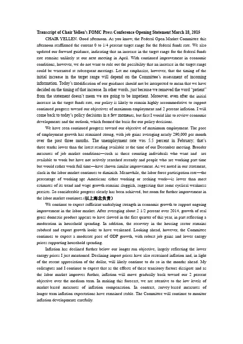
Transcript of Chair Yellen’s FOMC Press Conference Opening Statement March 18, 2015 CHAIR YELLEN. Good afternoon. As you know, the Federal Open Market Committee this afternoon reaffirmed the current 0 to 1/4 percent target range for the federal funds rate. We also updated our forward guidance, indicating that an increase in the target range for the federal funds rate remains unlikely at our next meeting in April. With continued improvement in economic conditions, however, we do not want to rule out the possibility that an increase in the target range could be warranted at subsequent meetings. Let me emphasize, however, that the timing of the initial increase in the target range will depend on the Committee’s assessment of incoming information. Today’s mo dification of our guidance should not be interpreted to mean that we have decided on the timing of that increase. In other words, just because we removed the word “patient” from the statement doesn’t mean we are going to be impatient. Moreover, even after the initial increase in the target funds rate, our policy is likely to remain highly accommodative to support continued progress toward our objectives of maximum employment and 2 percent inflation. I will come back to today’s policy decisions in a few mome nts, but first I would like to review economic developments and the outlook, which formed the basis for our policy decisions.We have seen continued progress toward our objective of maximum employment. The pace of employment growth has remained strong, with job gains averaging nearly 290,000 per month over the past three months. The unemployment rate was 5.5 percent in February; that’s three-tenths lower than the latest reading available at the time of our December meeting. Broader measures of job market conditions—such as those counting individuals who want and are available to work but have not actively searched recently and people who are working part time but would rather work full time—have shown similar improvement. As we noted in our statement, slack in the labor market continues to diminish. Meanwhile, the labor force participation rate—the percentage of working-age Americans either working or seeking work—is lower than most estimates of its trend and wage growth remains sluggish, suggesting that some cyclical weakness persists. So considerable progress clearly has been achieved, but room for further improvement in the labor market continues.(以上海北负责)We continue to expect sufficient underlying strength in economic growth to support ongoing improvement in the labor market. After averaging about 2-1/2 percent over 2014, growth of real gross domestic product appears to have slowed in the first quarter of this year, in part reflecting a moderation in household spending. In addition, the recovery in the housing sector remains subdued and export growth looks to have weakened. Looking ahead, however, the Committee continues to expect a moderate pace of GDP growth, with robust job gains and lower energy prices supporting household spending.Inflation has declined further below our longer-run objective, largely reflecting the lower energy prices I just mentioned. Declining import prices have also restrained inflation and, in light of the recent appreciation of the dollar, will likely continue to do so in the months ahead. My colleagues and I continue to expect that as the effects of these transitory factors dissipate and as the labor market improves further, inflation will move gradually back toward our 2 percent objective over the medium term. In making this forecast, we are attentive to the low levels of market-based measures of inflation compensation. In contrast, survey-based measures of longer-term inflation expectations have remained stable. The Committee will continue to monitor inflation developments carefully.This assessment of the outlook is reflected in the individual economic projections submitted for this meeting by the FOMC participants. As always, each participant’s projections are conditioned on his or her own view of appropriate monetary policy. The unemployment rate projections over the next few years and in the longer run are generally a bit lower than the December projections. At the end of this year, the central tendency for the unemployment rate stands at 5.0 to 5.2 percent, in line with participants’ estimates of the longer-run normal unemployment rate. Committee participants generally see the unemployment rate declining a little further over the course of 2016 and 2017. For economic growth, participants generally reduced their projections since December, with many citing a weaker outlook for net exports. Nonetheless, the central tendency of the growth projections for this year and next, at 2.3 to 2.7 percent, remains somewhat above estimates of the longer-run normal growth rate. Finally, FOMC participants project inflation to be quite low this year, largely reflecting lower energy and import prices. The central tendency of the inflation projections for this year is now below 1 percent, down noticeably since December. As the transitory factors holding down inflation abate, the central tendency rebounds to 1.7 to 1.9 percent next year and rises to 1.9 to 2.0 percent in 2017.(以上海东负责)Returning to monetary policy, as I noted at the outset, the Committee reaffirmed its view that the current 0 to 1/4 percent target range for the federal funds rate remains appropriate. But with economic conditions improving, and with further improvement expected in the months ahead, we have again modified our forward guidance. In December and January, the Committee judged that it could be patient in beginning to normalize the stance of monetary policy. That meant that we considered it unlikely that economic conditions would warrant an increase in the target range for the federal funds rate for at least the next couple of FOMC meetings. While it is still the case that we consider it unlikely that economic conditions will warrant an increase in the target range at the April meeting, such an increase could be warranted at any later meeting, depending on how the economy evolves.回到货币政策,就像我说的一样,委员会重申自己的观点,认为目前0至0.25%的联邦基准利率仍然是合适的。
For release on delivery10:00 a.m. EDTJuly 15, 2014Statement byJanet L. YellenChairBoard of Governors of the Federal Reserve Systembefore theCommittee on Banking, Housing, and Urban AffairsU.S. SenateJuly 15, 2014Chairman Johnson, Ranking Member Crapo, and members of the Committee, I am pleased to present the Federal Reserve’s semiannual Monetary Policy Report to the Congress. In my remarks today, I will discuss the current economic situation and outlook before turning to monetary policy. I will conclude with a few words about financial stability.Current Economic Situation and OutlookThe economy is continuing to make progress toward the Federal Reserve’s objectives of maximum employment and price stability.In the labor market, gains in total nonfarm payroll employment averaged about 230,000 per month over the first half of this year, a somewhat stronger pace than in 2013 and enough to bring the total increase in jobs during the economic recovery thus far to more than 9 million. The unemployment rate has fallen nearly 1-1/2 percentage points over the past year and stood at 6.1 percent in June, down about 4 percentage points from its peak. Broader measures of labor utilization have also registered notable improvements over the past year.Real gross domestic product (GDP) is estimated to have declined sharply in the first quarter. The decline appears to have resulted mostly from transitory factors, and a number of recent indicators of production and spending suggest that growth rebounded in the second quarter, but this bears close watching. The housing sector, however, has shown little recent progress. While this sector has recovered notably from its earlier trough, housing activity leveled off in the wake of last year’s increase in mortgage rates, and readings this year have, overall, continued to be disappointing.Although the economy continues to improve, the recovery is not yet complete. Even with the recent declines, the unemployment rate remains above Federal Open Market Committee (FOMC) participants’ estimates of its longer-run normal level. Labor force participation appears weaker than one would expect based on the aging of the population and the level ofunemployment. These and other indications that significant slack remains in labor markets are corroborated by the continued slow pace of growth in most measures of hourly compensation.Inflation has moved up in recent months but remains below the FOMC’s 2 percent objective for inflation over the longer run. The personal consumption expenditures (PCE) price index increased 1.8 percent over the 12 months through May. Pressures on food and energy prices account for some of the increase in PCE price inflation. Core inflation, which excludes food and energy prices, rose 1.5 percent. Most Committee participants project that both total and core inflation will be between 1-1/2 and 1-3/4 percent for this year as a whole.Although the decline in GDP in the first quarter led to some downgrading of our growth projections for this year, I and other FOMC participants continue to anticipate that economic activity will expand at a moderate pace over the next several years, supported by accommodative monetary policy, a waning drag from fiscal policy, the lagged effects of higher home prices and equity values, and strengthening foreign growth. The Committee sees the projected pace of economic growth as sufficient to support ongoing improvement in the labor market with further job gains, and the unemployment rate is anticipated to continue to decline toward its longer-run sustainable level. Consistent with the anticipated further recovery in the labor market, and given that longer-term inflation expectations appear to be well anchored, we expect inflation to move back toward our 2 percent objective over coming years.As always, considerable uncertainty surrounds our projections for economic growth, unemployment, and inflation. FOMC participants currently judge these risks to be nearly balanced but to warrant monitoring in the months ahead.Monetary PolicyI will now turn to monetary policy. The FOMC is committed to policies that promote maximum employment and price stability, consistent with our dual mandate from the Congress.Given the economic situation that I just described, we judge that a high degree of monetary policy accommodation remains appropriate. Consistent with that assessment, we have maintained the target range for the federal funds rate at 0 to 1/4 percent and have continued to rely on large-scale asset purchases and forward guidance about the future path of the federal funds rate to provide the appropriate level of support for the economy.In light of the cumulative progress toward maximum employment that has occurred since the inception of the Federal Reserve’s asset purchase program in September 2012 and the FOMC’s assessment that labor market conditions would continue to improve, the Committee has made measured reductions in the monthly pace of our asset purchases at each of our regular meetings this year. If incoming data continue to support our expectation of ongoing improvement in labor market conditions and inflation moving back toward 2 percent, the Committee likely will make further measured reductions in the pace of asset purchases at upcoming meetings, with purchases concluding after the October meeting. Even after the Committee ends these purchases, the Federal Reserve’s sizable holdings of longer-term securities will help maintain accommodative financial conditions, thus supporting further progress in returning employment and inflation to mandate-consistent levels.The Committee is also fostering accommodative financial conditions through forward guidance that provides greater clarity about our policy outlook and expectations for the future path of the federal funds rate. Since March, our postmeeting statements have included a description of the framework that is guiding our monetary policy decisions. Specifically, our decisions are and will be based on an assessment of the progress--both realized and expected--toward our objectives of maximum employment and 2 percent inflation. Our evaluation will not hinge on one or two factors, but rather will take into account a wide range of information,including measures of labor market conditions, indicators of inflation and long-term inflation expectations, and readings on financial developments.Based on its assessment of these factors, in June the Committee reiterated its expectation that the current target range for the federal funds rate likely will be appropriate for a considerable period after the asset purchase program ends, especially if projected inflation continues to run below the Committee’s 2 percent longer-run goal and provided that inflation expectations remain well anchored. In addition, we currently anticipate that even after employment and inflation are near mandate-consistent levels, economic conditions may, for some time, warrant keeping the federal funds rate below levels that the Committee views as normal in the longer run.Of course, the outlook for the economy and financial markets is never certain, and now is no exception. Therefore, the Committee’s decisions about the path of the federal funds rate remain dependent on our assessment of incoming information and the implications for the economic outlook. If the labor market continues to improve more quickly than anticipated by the Committee, resulting in faster convergence toward our dual objectives, then increases in the federal funds rate target likely would occur sooner and be more rapid than currently envisioned. Conversely, if economic performance is disappointing, then the future path of interest rates likely would be more accommodative than currently anticipated.The Committee remains confident that it has the tools it needs to raise short-term interest rates when the time is right and to achieve the desired level of short-term interest rates thereafter, even with the Federal Reserve’s elevated balance sheet. At our meetings this spring, we have been constructively working through the many issues associated with the eventual normalization of the stance and conduct of monetary policy. These ongoing discussions are a matter of prudent planning and do not imply any imminent change in the stance of monetary policy. TheCommittee will continue its discussions in upcoming meetings, and we expect to provide additional information later this year.Financial StabilityThe Committee recognizes that low interest rates may provide incentives for some investors to “reach for yield,” and those actions could increase vulnerabilities in the financial system to adverse events. While prices of real estate, equities, and corporate bonds have risen appreciably and valuation metrics have increased, they remain generally in line with historical norms. In some sectors, such as lower-rated corporate debt, valuations appear stretched and issuance has been brisk. Accordingly, we are closely monitoring developments in the leveraged loan market and are working to enhance the effectiveness of our supervisory guidance. More broadly, the financial sector has continued to become more resilient, as banks have continued to boost their capital and liquidity positions, and growth in wholesale short-term funding in financial markets has been modest.SummaryIn sum, since the February Monetary Policy Report, further important progress has been made in restoring the economy to health and in strengthening the financial system. Yet too many Americans remain unemployed, inflation remains below our longer-run objective, and not all of the necessary financial reform initiatives have been completed. The Federal Reserve remains committed to employing all of its resources and tools to achieve its macroeconomic objectives and to foster a stronger and more resilient financial system.Thank you. I would be pleased to take your questions.。
美联储新任主席耶伦:将在2014年秋季结束QE【秒读】美联储新任主席耶伦周四表示,继续减少资产采购项目规模,并且在2014年秋季的某个时间完全停止购买债券。
作为长期刺激措施的一部分,美联储目前每个月购买650亿美元国债和抵押贷款担保证券,相比项目启动时每个月850亿美元的规模要明显更低。
美国量化宽松货币政策退出对人民币价格和流动方向会有影响,国内股市、债市、房市都将承受巨大的压力。
美联储新任主席珍妮特-耶伦周四表示,恶劣的冬季天气可能对近期的经济数据表现有影响,但是她也重申自己的立场,那就是继续实施宽松货币政策应该是恰当的决策。
耶伦是在参加国会参议院银行事务委员会的听证会期间发表证词时提出这一看法的。
她说,“自我在众议院委员会听证会的发言以来,陆续发布的几组数据指向相比很多分析师所预测的更弱势的开支。
这种弱势表现的一部分反映了不利的天气状况,但是在目前这个阶段很难确定其程度。
”劳工部周四刚刚公布的数据显示,上周首次申请失业救济金的美国人数量有意外地小幅增长。
在耶伦发言的同时,美股指数继续上涨,而国债价格走势稳定。
耶伦女士在发言中说,紧缩财政政策已经对美国经济形成了拖累,同时也对货币政策有压制,“这种拖累效应可能在本财年内有显著的放松,但是也依然会是一种拖累。
同样,由于存在财政政策的拖累,对货币政策所形成的负担也是越来越大的。
”珍妮特-耶伦说,虽然她并不认为存在“大体上的泡沫担忧”,但是联储也确实在密切关注一些领域。
她表示,“比如,杠杆化贷款的承销标准明显是在恶化中,我们试图通过监管指引和特别的测试来加以解决,我们有这样的规管和监督工具。
”在谈到就业市场时,耶伦强调说,6.5%的失业率并不是联储所定义的充分就业,并称仅仅一个失业率数字并不足以用来判断劳动力市场的健康程度。
美联储在之前曾说,只要通货膨胀预期维持在2.5%之下,在失业率降低到6.5%以下之前都不会考虑加息。
珍妮特-耶伦在周四的听证会发言上说,“还有5%以上的人因为经济上的原因而只能接受兼职工作,这已经是劳动力人口中不寻常高的一个比例,我们还有很多美国人已经很长时间没有工作。
耶伦的经济政策观点——现代供给侧经济学用耶伦的话说,现代供给侧经济学旨在“通过增加劳动力供应、提高生产率、减少不平等和环境破坏来促进经济增长”。
这是美国财政部长珍妮特·耶伦(Janet L. Yellen)在斯坦福经济政策研究所2022年经济峰会上的讲话。
现代供给侧经济学旨在通过提高生产力的投资和促进劳动力供应的政策来扩大我们国家的经济潜力。
就总生产函数而言,这种方法通过更深层次的有形资本(包括公共资本和私人资本)提高劳动生产率;更高的人力资本;以及科学技术的进步。
此外,基于税收的激励措施和亲家庭的劳动政策旨在提高劳动力参与率。
相比之下,传统的供给侧经济学主要侧重于通过降低资本使用成本的政策来增加私人资本存量,主要是通过减税投资。
除了关注更广泛的生产要素外,现代供给侧经济学还关注跨部门、跨人员和跨地方的投资分配。
在传统方法下,降低资本使用成本的减税通常首先使资本所有者受益;如果这些削减导致更广泛的投资,那么这些好处就会更广泛地传播——这是一个有争议的假设。
尽管去年面临金融环境收紧和全球经济不确定性加剧,但美国金融体系仍然具有弹性。
美国银行体系整体健全,拥有强大的资本和流动性状况。
——更高的利率对国家有利这位前美联储主席表示,总统的计划每年将总额约为4000亿美元,她认为这一支出水平不足以造成通胀超支。
“如果我们最终的利率环境略高,这实际上对社会观点和美联储的观点来说都是一个加分项,”耶伦告诉彭博社。
“十年来,我们一直在与过低的通货膨胀和过低的利率作斗争,”她说。
她补充说,如果这些一揽子计划有助于“缓解问题,那么这不是一件坏事——这是一件好事。
——有弹性的消费者阻止了经济衰退出人意料的有弹性的美国消费者阻止了经济衰退——现在美联储可以在更长时间内保持较高的利率。
美国财政部长珍妮特·耶伦(Janet Yellen)表示,尽管有经济衰退预测,但美国经济“已被证明比预期更具弹性”,并表示希望该国能够在保持劳动力市场强劲的同时降低通胀。

鲍威尔在当前可谓腹背受敌。
前有特朗普的指摘,后有金融机构和媒体的压力。
在Jackson Hole 会议的开场演讲中,他明智地选择了回避这种双重压力。
在鲍威尔Jackson Hole的发言以前,纽约联储刚刚公布了美联储对一级交易商(一级交易商名单中包括几乎所有的大型投资银行)以及市场参与者(市场参与者名单中包括贝莱德、先锋基金、摩根大通资管等大型资管企业)在内的金融机构的调查问卷。
问卷显示,他们对美联储的市场沟通感到非常困惑。
没有一家一级交易商认为美联储的沟通“非常有效”,二十四家受调查的一级交易商中,仅有一家认为美联储的沟通“比较有效”,八家认为“中规中矩”,十一家认为“很不有效”,四家认为“沟通无(低)效”。
仅有一家市场参与者认为美联储的沟通“非常有效”,二十八家受调查的市场参与者中,八家认为美联储的沟通“比较有效”,五家家认为“中规中矩”,七家认为“很不有效”,七家认为“沟通无(低)效”。
根据他们的表态来看,美联储的表态有时间不一致的问题,此外也不够明晰,令人困惑,官员之间的分歧也导致了不一致性。
要知道,这份调查问卷先于FOMC的7月会议,也就意味着在7月底议息会议后灾难性的发布会表现以前,市场已经对美联储和鲍威尔所传达的信息感到相当困惑了。
鲍威尔在当前可谓腹背受敌。
前有特朗普的指摘,后有金融机构和媒体的压力。
似乎已经没有人在支持他治下的美联储了,美联储内部也出现了持有异见的官员。
我们在之前的文章中曾提到:现任美联储主席鲍威尔正在犯一个严重的错误——即他误以为更多且更频繁的表达是美联储沟通政策上的进步,此外,为了避免产生政策上的“道德风险”,他在很多应该明晰表态的问题上又表现得过于晦涩。
结果造成了当下非常混乱的结果——美联储与市场之间无法就当下的经济环境认知达成共识,对于未来的利率路径也无法达成共识,且这种分歧的影响在加强。
许多观察者认为,美联储被市场和总统“绑架”了,但在笔者看来,这纯粹是鲍威尔作茧自缚的结果。

张津镭;耶伦听证会全线压迫美元
耶伦将会在周四(11月14日)在美国参议院银行业委员会致辞,一份关于其陈词的复印件被媒体提前得到。
据稿件内显示,美联储(FED)副主席耶伦(JanetYellen)认为美国通胀率料将在一段时期内低于美联储2%的通胀目标。
同时,她在讲稿中并未过多提及对美联储货币政策或美国经济的看法,称支持经济复苏是货币政策更加正常“最为确信的途径”,美国失业率抬高,就业市场和经济表现“远低于”潜在水平;当制定和实施货币政策时,美联储将金融稳定性目标纳入考量。
耶伦指出,当制定新规则时,美联储应当限制对社区银行和小型机构的监管负担,在解决银行业大而不能倒问题上,资本和流动性规则是重要的工具;美国监管方已经在解决金融系统疲软问题上采取大量行动,前面还有工作要做。
耶伦强烈支持美联储在传导机制上的承诺,称若被确认为美联储主席,将继续这样做;承诺将利用美联储监督和监管权力,来降低下一轮金融危机的威胁。
这些陈述爆光后市场的反应:
美元下跌-全线下挫大约25-50点
贵金属反弹–黄金上涨8-10美元
美债走高–10年期殖利率下跌3.1个基点。

叶大干:美联储将会扩大QE的规模?William English和David Wilcox是美联储货币政策分析和宏观经济方面最资深的经济学家,并发表了两份独立的研究报告。
报告显示,美联储很有可能调降首次加息的失业率门槛。
我们已经产生这种观点已经有相当长的时间了,但是并不确定这种事情是否会发生。
虽然美联储近期政策仍存在相当大的不确定性,但是我们现在认为,美联储将于2014年3月份的FOMC会议上把加息的失业率门槛从6.5%调降至6.0%;美联储届时还将宣布开始削减QE。
美联储也可能在2013年12月份降低加息的失业率门槛。
若果真如此,那么美联储更早削减QE的几率也会上升。
高盛经济学家Hatzius认为,美联储将把加息的失业率门槛从6.5%调降至6.0%,这意味着美联储将在更长时期内维持宽松政策。
就目前这两份报告来看,美联储大部分官员还是更加倾向于进一步扩大宽松规模来刺激经济的。
美国目前的实际经济状况比潜在增长是差很多的,特别是上两个月的美国债务上限问题和美国政府关门事件,对美国经济的打击也是有一定的影响的。
还有一个值得我们关注的事件就是如果耶伦正式上台后,她所倡导的“最优控制”理论是需要“将要不负责任的可靠承诺”,这几个理由都给出了支持美联储进一步宽松政策的理由。
不过就报告而言,我们都可以清楚看到美联储对于缩减QE的问题至少要到2014年3月份才会给出比较明确的决定。
换言之,美联储将加强前瞻指引。
这两份报告没有讨论QE;相反报告指出“(QE)的成本和效率存在的不确定性,导致减少购债的水平”。
这种讨论并不能给到我们很多,但这与以下观点一致,那就是美联储降低加息的失业率门槛同时还会削减QE。
不过目前,我们应该清楚认识到,美联储可能进一步扩大宽松政策的规模也是非常大的可能性的!。
叶大干:怎么看待美联储主席耶伦的听证会美联储主席耶伦(Janet Yellen)周四(2月27日)将重返美国国会山,在参议院银行委员会面前就经济前景及货币政策进行演讲。
若按照此前众议院的安排方式,在今晚23:00耶伦进行证词演讲前,其演讲稿会在21:00提前发布,需要给予关注。
在此前2月11日的众议院听证会上,耶伦基本延续了前任伯南克的施政方略,暗示美联储将继续信守“逐渐放慢购债步伐”的承诺,不过仍巧妙地加上了“假设性条件”。
近期美国数据虽然整体疲软,贵金属也乘机上涨不少,不过美元指数并没有大幅下挫,反而目前还比较稳定再80关口一带的位置,而美股方面也没有受到太大的影响,也是有不错的表现。
美国方面一旦出现比较利好的消息,那么美指会得到较好的支撑,而贵金属和非美货币反而会有比较强的打压。
2月26日晚间的美国1月新屋销售创五年多新高,环比大增9.6%,就大大提振了美元指数,而黄金和白银相继都下跌了不少。
昨日的市场整体表现为道指涨0.1%,特斯拉盘中涨7%,白银期货价格大幅下挫3.5%,黄金期货大跌1.3%。
而技术面看来贵金属目前也是短线承压,不过中线的一个上涨形态依然还是存在,美国数据方面的影响会给这个走势有一定的指引的。
个人看了一些关于近期市场的数据统计以及一些投行的投资思路,市场上对于美联储继续缩减QE的态度还是比较肯定的,前提就是美国经济如期恢复和发展。
今晚的听证会估计也是没有比较大的新意的,美联储会继续呈现一些鹰派的思路,也许会是一些比较委婉一些的话语,同时也会有一些对于中国和日本市场经济的一些夸大词语,但是近期美国比较疲软的这些经济数据并不能影响整个美联储季度的经济计划。
或许今晚我们依然还是可以看到美联储主席耶伦继续打太极的一面,美联储的一向作风就是喜欢夸大别人,贬低自己,背地里又搞一套的。
美联储主席耶伦演讲全文美联储主席耶伦演讲全文美联储9月17日宣布暂不启动加息,维持关键利率在0-0.25%不变。
北京时间凌晨2点30分,美联储主席珍妮特·耶伦(Janet L. Yellen)准时亮相新闻发布会。
她表示:其他国家的发展可能会对美国经济活动有所抑制,并可能在短期时间内进一步给通胀带来下行压力。
鉴于美国与世界其他地区在经济和金融活动方面联系密切,国外形势值得密切关注。
值得一提的是,耶伦强调,10月份仍然有行动的可能,美联储在必要情况下可以召开特别记者会。
这意味着,不少机构“没有发布会就不会加息”的判断,并不成立。
按照美联储安排,将于10月27-28日举行的下一次美联储议息会议,并没有发布会,12月举行的年内最后一次会议才有。
耶伦同时表示,大衰退中的经济复苏已经足够充分,而国内消费也似乎足够强劲,这些为9月加息提供理由,但鉴于全国其他经济体的高度不确定性和通胀预期小幅走软,委员会判断此时应当等待更多的证据,包括进一步改善劳动力市场,以提高对中期通胀将逐步增长到2%的信心。
由于美联储在9月并未启动加息,耶伦的本次讲话,成为今后一段时间,市场所能听到的来自美联储决策层的最权威声音。
按照既定安排,美联储年内还有两次货币政策会议可决定是否加息,时间分别为10月和12月。
以下是耶伦在新闻发布会上的讲话要点:为何9月不加息今天的政策决定获得了巨大关注。
大衰退中的经济复苏已经足够充分,而国内消费也似乎足够强劲,以上观点为此时加息提供理由。
我们在会上讨论了加息的可能性。
但是,鉴于外国经济体的高度不确定性和通胀预期小幅走软,委员会判断此时应当等待更多的证据,包括进一步改善劳动力市场,以提高对中期通胀将逐步增长到2%的信心。
现在,我不想夸大近期发展的影响。
这未从根本上改变了我们的预期。
经济运行一直良好。
我们希望可以持续。
耶伦认为,如果美联储等太久才加息,经济可能会过热。
急刹车并非好的政策,可能有导致经济下滑的可能。
中国如何应对美国量化货币宽松政策作者:李莹来源:《财经界·学术版》2013年第03期摘要:美国最近五年来采取了三轮量化货币政策,保证本国经济的持续发展与政策的稳定。
这种非常规的做法将会对中国的经济产生严重的危害。
本文阐述美国量化货币政策采取的具体措施,分析这种政策会对中国经济可能造成的影响,并提出相对应的解决措施。
关键词:量化货币宽松政策经济影响解决措施美国为了保持本国的经济利益,在2009年3月18日宣布实行第一轮的量化货币宽松政策(Quantitative Easing),随后在2010年11月3日与2012年9月14日进行了二轮与三轮的量化货币宽松政策的实行,这三轮的量化货币宽松政策,对于中国新兴的市场经济体制产生极大的冲击,因此,中国必须采取相应的措施来化解美国量化货币宽松政策所造成的危机。
一、美国实行量化货币宽松政策的原因对于美国来说,实行量化货币宽松政策主要有三个方面的原因:第一,避免美国通货紧缩现象的发生,甚至通过这一政策的实施来实现通货膨胀,降低美国本土的实际利率,避免经济的衰退。
第二,在这种政策的影响下,银行可以有充足的资金保证行业内部的流动性,保障金融体系的正常运转,鼓励银行积极进行货币的放贷。
第三,通过货币宽松政策,使国家利率保持低位水平,从而能有有效的降低公司贷款的成本,促进国民消费,达到经济复苏的目的。
根据调查统计的结果表明,美国通过量化货币宽松政策,成功地促进国家基础货币的增加,并减轻国民与本土企业的负债压力,缓解美国市场陷入经济衰退的领域。
这种政策,一方面加强金融市场的资金流动性,银行放贷意愿得到提高,放贷市场逐步复苏;另一方面,降低企业与个人借贷的成本,促进消费,提高企业的借贷需求。
二、量化货币政策对中国造成的经济影响中国作为世界三大经济体之一,不可避免的受到美国量化货币政策的影响,而其中消极影响占据绝大多数,总体表现有以下几个方面:(一)加重了中国通货膨胀的压力由于美国量化货币宽松政策,造成美元的相对贬值与泛滥,削弱了美元对于国际资产的吸引力;与此同时,人民币由于不断升值,从而使大量的国际资产涌进中国,加重了这种通货膨胀的压力。
叶大干:耶伦听证会我们要做好什么准备?
美联储提名主席耶伦(Janet Yellen)的证词内容提前泄露,暗示美国就业市场复苏力度不足以让美联储开始回收每月购债行动。
耶伦指出,美国经济的强势复苏终将推动美联储缩减货币政策的适应性,并减少对资产购置等非常规货币政策的依赖。
金融危机的爆发距今已有多年,但美国经济仍有很长的路要走。
“我认为美联储在实现工作目标方面已取得了极大进展,但仍有很多工作要做。
”
从耶伦以往的演讲中可以发现,“最优控制”方法占据着举足轻重的地位。
在“最优控制”的前提下,美联储可以用模型计算短期利率的最优路径,只要失业率相较通胀离目标更远,政策制定者就可以保持低利率,尽管如此一来通胀可能会稍微高于目标。
众所周知,耶伦是美联储鸽派阵营代表人物,因此任何偏离鸽派内容的讲话都会改变现有的市场预期。
那么我们所要留意的词眼或者注意的问题在哪里呢?一方面要留意耶伦是否会在听证会上对货币政策重新定义或者有新的计划,特别是对于美联储退出或者缩减QE这个计划是否会重新定义。
另外一方面对于耶伦是否会提出相关词语,退出并不意味着政策紧缩,那么预计债券收益率会走高,没有利率也会回升。
不过相对于黄金的走势,我们就要留意1300这个关口的突破情况。
如果耶伦坚持她的鸽派思维,那么黄金站上1300的可能性是很大的,如果耶伦转为鹰派思维,那么黄金是
很大几率继续下跌至上月低位1252,甚至是1230!就目前技术面来看,我更加期待后者的走势。
耶伦将于稍后的北京时间23:00面对参院银行业委员会(Senate Banking Committee)发表证词,若耶伦顺利获得国会认可,那么她将成为历史上首位女性美联储主席。
《金融发展研究》第9期非均衡复苏下的货币政策调整杰罗姆·鲍威尔王宇译收稿日期:2021-09-07作者简介:作者杰罗姆·鲍威尔(Jerome Powell )为美国联邦储备委员会主席;译者为中国人民银行研究局研究员王宇博士。
本文是作者在2021年8月27日在杰克逊霍尔会议上的讲话,译者于2021年8月31日完成翻译。
文章标题和文中标题为译者所加。
摘要:实现充分就业和物价稳定是美联储货币政策的坚定目标。
当前,美国劳动力市场持续好转,就业稳步恢复,但长期失业率仍然居高不下,劳动力市场依然疲软。
与此同时,随着美国经济的快速复苏,通货膨胀急剧上升。
然而,根据美联储评估情况可知,全面通货膨胀尚未形成,长期通货膨胀预期基本稳定,此轮通货膨胀是暂时的,历史经验表明,如果为了应对暂时性通货膨胀而收紧货币政策可能弊大于利。
因此,美联储将继续实施当前资产购买计划,直到充分就业和物价稳定取得实质性进展。
但即使结束该计划,美联储仍将继续支持宽松的金融环境,未来减少资产购买也不是加息的信号。
关键词:复苏;货币政策;充分就业;通货膨胀;资产购买计划中图分类号:F830文献标识码:B 文章编号:1674-2265(2021)09-0042-04DOI :10.19647/ki.37-1462/f.2021.09.005自美国经济受到新冠肺炎疫情的全面冲击,如今已经17个月。
为遏制疫情蔓延,大部分经济部门被迫关闭,经济出现了前所未有的衰退。
复苏之路艰难而曲折。
要感谢奋战在抗击新冠肺炎疫情第一线的人们:那些维持经济运转的工人,那些关心和照顾身处困难者的人,以及那些日夜工作在医学研究、商业领域和政府部门的人。
他们争分夺秒,齐心协力,研发、生产、分发和接种疫苗。
我们也要记住那些受新冠肺炎疫情感染而失去生命的人,以及他们的亲人。
力度空前的宏观政策,支持了此次非均衡复苏,使其在许多方面都表现出与以往不同的特征。
具体表现为,在经济下行时期,个人总收入不降反升,家庭支出从服务业部门转向制造业部门等。
哥伦比亚大学蒙代尔教授演讲全文(2004-05-31)尊敬的纪校长,女士们,先生们:非常高兴参加这次论坛,我注意到今天来的都是各自领域非常有名的人士,我相信你们在今天讨论中将给出自己卓越独特的见解。
今天我要谈的是中国的人民币汇率问题。
下面这个表格是关于中国和美国的经济增长速度的对比表格,我们看到中国和美国经济增长速度是很快的,中国经济增长速度尤其快,89、90年增长的速度很高。
这些是关于美国、日本、欧元区通货膨胀率的数据的表格,中国经济的增长速度非常快,但是90年代通货膨胀率是相对比较高的。
这个表格就是刚才说的四个地区通货膨胀率的水平。
我们可以看到这条线是中国通货膨胀的情况,上世纪90年代中国是通货紧缩的情况,现在是向零发展,未来可能突破零达到3.5%通货膨胀的水平,但是我们不能够把通货膨胀和物价的上涨和经济过热联系起来,因为中国的货币是钉住美元的,如果美元贬值了,就会导致以人民币计价的物价水平的上升,如果美元能够升值的话中国通货膨胀也会随之下降。
世界上有许多国家把本国货币钉住美元,在这种情况下如果美元贬值的话,本国就会出现物价上涨情况,美元升值本国物价就会下跌,如果把这种情况作为严重的经济问题,做出经济过热的判断,我们就犯了错误了,是不应该这么认为。
所以我们不应该因为出现物价上涨就认为中国经济过热,情况不是这样的,我们应该更加关注其他根本的问题,如电力问题,能源问题,不仅仅关注由于美元挂钩的问题产生的物价上涨。
为什么我强调这个问题,因为中国是否存在经济过热关系着我们是否认为人民币应该升值,如果经济过热那么让人民币升值就有它的道理了,但是这种说法是没有理由的。
我们可以看到在去年,7国集团召开会议的时候,人们谴责中国输出通货紧缩,而不过一个月时间《纽约时报》又在谴责中国是通货膨胀,可以看出对人民币汇率的问题大家看法不一样。
中国在这个问题上受到七大工业国的非常大压力,要求人民币升值。
关于亚洲区的货币--亚元的说法,在这儿我给大家一个世界货币地图。
For release on delivery7:15 p.m. EDTApril 11, 2012The Economic Outlook and Monetary PolicyRemarks byJanet L. YellenVice ChairBoard of Governors of the Federal Reserve SystemAt theMoney Marketeers of New York UniversityNew York, New YorkApril 11, 2012I appreciate the opportunity to speak with you this evening. The Money Marketeers are renowned for their keen interest in the economy and monetary policy. With that in mind, I’ll describe how my views concerning the stance of monetary policy relate to my assessment of the economic outlook. As you know, the Federal Open Market Committee (FOMC) issued statements following its January and March meetings indicating that it “currently anticipates that economic conditions--including low rates of resource utilization and a subdued outlook for inflation over the medium run--are likely to warrant exceptionally low levels for the federal funds rate at least through late 2014.”I agreed with those judgments and, in my remarks tonight, I’ll explain my views and describe some of the analytical tools that I use in making such policy decisions. I will also discuss the conditional nature of the Committee’s policy stance. Let me emphasize at the outset that the remainder of my remarks reflect my own views and not those of others in the Federal Reserve System.1The Labor Market and the Economic OutlookI will start by describing current conditions and key features of the economic outlook that influence my views on the appropriate stance of monetary policy. To summarize, the labor market has shown welcome signs of improvement. Even so, the economy remains far from full employment. Furthermore, the improvement in labor market conditions has outpaced the seemingly moderate growth of output. Looking ahead, significant headwinds are likely to continue to restrain aggregate spending, and progress in closing the remaining employment gap is likely to be quite gradual. Apart1 I appreciate assistance from members of the Board staff--James Clouse, William English, Michael Leahy, David Lebow, Andrew Levin, Andrea Lowe, Steven Meyer, and David Reifschneider--who contributed to the preparation of these remarks.from sizable increases in gasoline prices, inflation has been subdued in recent months. While the jump in energy prices is pushing up inflation temporarily, I anticipate that subsequently inflation will run at or below the Committee’s 2 percent objective for the foreseeable future. Let’s examine the economic outlook in greater detail before considering how that outlook shapes my views on appropriate policy.Starting with the labor market, as I mentioned, there have been encouraging signs of improvement in recent months. The unemployment rate had hovered around 9 percent for much of last year but moved down in the fall and averaged 8-1/4 percent in the first three months of this year, about 1-3/4 percentage points lower than its peak during the recession. And even though the latest employment report was somewhat disappointing, private sector payrolls expanded, on average, by about 210,000 per month in the first quarter, up from gains averaging around 150,000 per month during most of 2011. Other labor market indicators have shown similar improvement.This news is certainly welcome, yet it must be kept in perspective. Our economy is recovering from the steepest and most prolonged economic downturn since the 1930s, and these job gains still leave us far short of where we need to be. The level of private payrolls remains nearly 5 million below its pre-recession peak, and the unemployment rate stands well above levels that I, and most analysts, judge as normal over the longer run.Figure 1 shows the unemployment rate together with the outlook of professional forecasters from last month’s Blue Chip survey.2 The solid blue line shows the Blue2 The Blue Chip survey provides forecasts on a quarterly basis only through the end of 2013. To construct quarterly forecasts for 2014, we interpolate the annual projections reported in the March survey. AccordingChip consensus and the blue shading denotes the range between the top 10 and bottom 10 projections of forecasters in the March Blue Chip survey. The figure also shows the central tendency of the unemployment projections that my FOMC colleagues and I made at our January meeting: Those projections reflect our assessments of the economic outlook given our own individual judgments about the appropriate path of monetary policy. As in the Blue Chip consensus outlook, FOMC participants’ projections indicate that unemployment will decline gradually from current levels. Included in the figure as well is the central tendency of FOMC participants’ estimates of the longer-run normal unemployment rate, which ranges from 5.2 percent to 6 percent. The unemployment rate is expected to remain well above its longer-run normal value over the next several years.As you know, economic forecasts always entail considerable uncertainty. Figure 2 illustrates the degree of uncertainty surrounding projections of unemployment. The gray shading denotes a model-based 70 percent confidence interval for the unemployment rate, based on the sorts of shocks that have hit the economy over the past 40 years.3 Judging from historical experience, the consensus projection could be quite far off, in either direction. That said, the figure also shows that labor market slack at present is so large that even a very large and favorable forecast error would not change the conclusion that slack will likely remain substantial for quite some time.to the April edition of the Blue Chip survey, which was released yesterday, “The con sensus outlook for U.S. economic growth this year and next underwent minimal change over the past month.”3The forecast confidence interval is generated using stochastic simulations of the Federal Reserve staff’s FRB/US model. Specifically, a baseline is constructed centered on the midpoint of the central tendency of the FOMC’s projections released in January, and then the model is repeatedly simulated with shocks drawn randomly for the set of historical disturbances experienced over the period from 1968 to 2011. Similar estimates of forecast confidence intervals would be obtained if the intervals were instead constructed using the actual historical forecasting errors of private forecasters; for further discussion, see Table 2 of the FOMC’s Summary of Ec onomic Projections.Some observers question just how large the shortfall from full employment really is and hence worry that further increases in aggregate demand could push up inflation. Their concern is that a large part of the rise in unemployment since 2007 is structural rather than cyclical. I agree that the magnitude of structural unemployment is uncertain, but I read the evidence as supporting the view that the bulk of the rise in unemployment that we saw in recent years was cyclical, not structural in nature. Assessments concerning the degree of slack in the labor market are highly relevant to an evaluation of the appropriate stance of policy, so I’d like to review my reasoning in some detail.First, the fact that the rise in unemployment was quite widespread across industry and occupation groups casts doubt on the hypothesis that there has been an unusually large mismatch between the types of job vacancies and the types of workers available to fill them. Certainly, job losses in the construction sector and in financial services were particularly sharp--not surprising given the collapse in the housing market and in the financial sector that we saw in 2008--but so were losses in manufacturing and other highly cyclical industries that typically are hit especially hard in recessions. Indeed, measures of the dispersion of employment changes across industries did not increase more than past experience would have predicted given the depth of the recession.Some commentators have noted that “house lock”--the reluctance or inability of homeowners to sell in a declining price environment or when underwater on their mortgages--may be preventing people from moving to find available jobs in new locations. However, evidence from migration patterns suggests that house lock is not having a significant effect on the level of structural unemployment. While migration within the United States has been trending down for some time, the reduction in mobilityduring the recession was not greater for homeowners than for renters, nor was it especially pronounced for areas where housing prices have declined the most and so where house lock would likely be most prevalent.4Finally, I do not interpret data suggesting an outward shift in the Beveridge curve as providing much evidence in favor of an increase in structural unemployment. The Beveridge curve plots the relationship between unemployment and job vacancies. Cyclical variations in aggregate demand tend to move unemployment and job vacancies in opposite directions, whereas structural shifts would be expected to move vacancies and unemployment in the same direction. For instance, a structural mismatch between businesses’ hiring needs and the skills of unemployed workers would tend to push up the level of vacancies for a given level of unemployment. Figure 3 plots the co-movement of unemployment and job vacancy rates since 2007.5 Consistent with a substantial decline in aggregate demand, followed by some modest recovery, movements in unemployment and vacancies since 2007 display a predominantly inverse relationship. However, figure 3 shows that as job vacancies have risen during the recovery, unemployment has declined by less than might have been expected based on the relationship that prevailed during the contraction. This outcome has led some to suggest that the Beveridge curve has shifted outward, reflecting an increase in the extent of job mismatch. In my view, a portion of this apparent outward shift in the Beveridge curve reflects increases in the maximum duration of unemployment benefits, which have been important in buffering the effects of 4 See Raven Molloy, Christopher L. Smit h, and Abigail Wozniak (2011), “Internal Migration in the United States,” Finance and Economics Discussion Series 2011-30 (Washington: Board of Governors of the Federal Reserve System, May), /pubs/feds/2011/201130/201130pap.pdf.5 The measure of job vacancies shown in figure 3 is derived from indexes of help-wanted advertising published by the Conference Board. Print and online indexes are combined as in Regis Barnichon (2010), “Building a Composite Help-Wanted Index,” Economics Letters, vol. 109 (December), pp. 175-78.the weak labor market on workers and their families. The influence of these benefits will dissipate as they are phased out and the economy recovers. In addition, loop-like movements around the Beveridge curve are common during recoveries. Vacancies typically adjust more quickly than unemployment to changes in labor demand, causing counterclockwise movements in vacancy-unemployment space that can look like shifts in the Beveridge curve. Figure 4 plots the relationship seen during and after the 1973 and 1982 recessions alongside the current episode. As can be seen, such counterclockwise movements also occurred during these two earlier deep recessions.6While I do not see much evidence of any significant increase in structural unemployment so far, I am concerned that structural unemployment could increase over time if the labor market heals too slowly--a phenomenon known as hysteresis. An exceptionally large fraction of those now unemployed--more than 40 percent--have been out of work for six months or more. My concern is that individuals with such long unemployment spells could become less employable as their skills deteriorate and as they lose their connections to the labor market. This outcome does not appear to have occurred in the wake of previous U.S. recessions, but the fraction of the unemployed who have been out of work for a long period is much higher now than it has been in the past. To date, I have not seen evidence that hysteresis is occurring to any substantial degree. For example, the probability of finding a new job has not deteriorated more for individuals experiencing a long-term bout of unemployment relative to those facing6 See John Lindner and Murat Tasci (2010), “Has the Beveridge Curve Shifted?”Economic Trends (Cleveland: Federal Reserve Bank of Cleveland, August),/research/trends/2010/0810/02labmar.cfm; and Rob Valletta and Katherine Kuang (2010), “Is Structural Unemployment on the Rise?”FRBSF Economic Letter 2010-34 (San Francisco: Federal Reserve Bank of San Francisco, November),/publications/economics/letter/2010/el2010-34.html.shorter spells. Nonetheless, the risk that continued high unemployment could eventually lead to more-persistent structural problems underscores the case for maintaining a highly accommodative stance of monetary policy.Putting all the evidence together, I see no good reason to doubt that our nation’s high unemployment rate indicates a substantial degree of slack in the labor market. Moreover, while I recognize the significant uncertainty surrounding such forecasts, I anticipate that growth in real gross domestic product (GDP) will be sufficient to lower unemployment only gradually from this point forward, in part because substantial headwinds continue to restrain the recovery.One headwind comes from the housing sector, which has typically been a driver of business cycle recoveries. We have seen some improvement recently, but demand for housing is likely to pick up only gradually given still-elevated unemployment, uncertainties over the direction of house prices, and mortgage credit availability that seems likely to remain very restricted for all but the most creditworthy buyers. When housing demand does pick up more noticeably, the huge overhang of both unoccupied dwellings and homes in the foreclosure pipeline will likely allow demand to be met for a time without a sizable expansion in homebuilding.A second headwind comes from fiscal policy. State and local governments continue to face extremely tight budget situations in light of the weak economy, depressed home prices, and the phasing out of federal stimulus grants, though overall tax revenues have been improving and that should continue as the economy expands further. At the federal level, stimulus-related policies are scheduled to wind down, while both realdefense and nondefense purchases are expected to decline over the next several years under the spending caps put in place last year.A third factor weighing on the outlook is the sluggish pace of economic growth abroad. Strains in global financial markets have eased somewhat since late last year, an improvement that reflects in part policy actions taken by European authorities. Nonetheless, risk premiums on sovereign debt and other securities are still elevated in many European countries, while European banks continue to face pressure to shrink their balance sheets, and concerns about the outlook for the region remain. A further slowdown in economic activity in Europe and in other foreign economies would inhibit U.S. export growth.For these reasons, I anticipate that the U.S. economy will continue to recover only gradually and that labor market slack will remain substantial for a number of years to come.One consideration that further complicates this outlook is the inconsistency between recent movements in economic growth and employment: Unemployment has declined significantly over the past year even though growth appears to have been only moderate. This unanticipated decline in the unemployment rate presents something of a puzzle, and it creates uncertainties for the outlook and policy.To illustrate this puzzle, figure 5 plots changes in the unemployment rate against real GDP growth--a simple portrayal of the relationship known as Okun’s law. It is evident from the figure that 2011 is something of an outlier, with the drop in the unemployment rate last year much larger than would seem consistent with real GDP growth below 2 percent. One possibility, highlighted by Chairman Bernanke in a recentspeech, is that last year’s decline in unemployment represents a catch-up from the especially large job losses during late 2008 and 2009.7 According to this hypothesis, employers slashed employment especially sharply during the recession, perhaps out of concern that the contraction could become even more severe; in particular, the figure shows that in 2009, the unemployment rate rose by considerably more than the decline in GDP would have suggested. Then, last year, employers may have become confident enough in the recovery to increase hiring and relieve the unsustainable strain that the earlier cutbacks had placed on their workforces. I think the evidence is consistent with this hypothesis, and I have incorporated it into my own modal forecast.If last year’s Okun’s law puzzle was largely the result of such a catch-up in hiring, I would expect progress on the unemployment front to diminish unless the pace of GDP growth picks up. After all, catch-up can go on for only so long. Of course, there are other conceivable explanations for this puzzle, including some that would point to a faster decline in unemployment in coming years. For example, GDP could have risen more rapidly over the past year than current data indicate. It will be important to pay close attention to indicators of both the labor market and GDP to try to gauge the likely pace of improvement in economic activity going forward and, hence, the appropriate stance of monetary policy over time.Let me now turn to inflation. Overall consumer price inflation has fluctuated quite a bit in recent years, largely reflecting movements in prices for oil and other commodities. For example, inflation moved up in the first part of 2011 as a rise in the7See Ben S. Bernanke (2012), “Recent Developments in the Labor Market,” speech delivered a t the National Association for Business Economics Annual Conference, Washington, March 26,/newsevents/speech/bernanke20120326a.htm.price of oil and other commodities fed through to gasoline prices, and, to a lesser extent, to prices of other goods and services. Then inflation subsided after commodity prices came off their peaks. More recently, prices of crude oil, and thus of gasoline, have turned up again. But smoothing through these fluctuations, inflation as measured by the personal consumption expenditures (PCE) price index averaged 2 percent over the past two years. Using the price index excluding food and energy--another rough way to abstract from transitory fluctuations--inflation averaged about 1-1/2 percent over the past two years. These rates are lower than the inflation rates that were seen prior to the recession, and they are at or below the FOMC’s long-run goal of 2 percent inflation.In my view, the subdued inflation environment largely reflects two factors. First, the substantial slack in the labor market has restrained inflation by holding down labor costs. Second, and of critical importance, longer-term inflation expectations have been remarkably stable. Like many other observers, I was concerned that inflation expectations might move lower during the recession, driving down both wages and prices in a self-reinforcing spiral. The Federal Reserve acted forcefully to resist such an outcome and, fortunately, that destructive dynamic did not take hold. Indeed, the stability of expectations has meant that the price increases driven by costs of oil and other commodities have had only temporary effects on the rate of inflation. Although firms passed higher input costs into their prices when they could do so, those one-time price increases have not led to an expectations-driven process that might have resulted in persistently higher inflation.The same key factors that have kept core inflation subdued provide the rationale for my inflation forecast. I anticipate that slack in the labor market will continue torestrain growth in labor costs and prices. And, given the stability of inflation expectations, I expect that the latest round of gasoline price increases will also have only a temporary effect on overall inflation. Indeed, if crude oil prices were to follow the downward-sloping path implied by current futures contracts, energy costs would serve as a restraining influence on overall inflation over the next several years. Figure 6 presents the central tendency of FOMC participants’ pr ojections of inflation at the time of our January meeting. Most expected inflation to be at, or a bit below, our long-run objective of 2 percent through 2014; most private forecasters also appear to expect inflation by this measure to be close to 2 percent.8 As with unemployment, uncertainty around the inflation projection is substantial.Benchmarks for Assessing Monetary Policy: Optimal ControlAs I indicated at the outset of my remarks, I supported the Committee’s statements in January and March pertaining to the stance of monetary policy. I will now explain the rationale for my judgments, and I will describe some of the tools that I use to make such assessments. I consider it essential, in making judgments about the stance of policy, to recognize at the outset the limits of our understanding regarding the dynamics of the economy and the transmission of monetary policy. Because I see no magic bullet for determining the “right” stance of policy, I commonly consider a number of different approaches.One approach I find helpful in judging an appropriate path for policy is based on optimal control techniques. Optimal control can be used, under certain assumptions, to 8 The Blue Chip survey reports inflation forecasts for the consumer price index (CPI), not the PCE price index. However, the Survey of Professional Forecasters (SPF) provides forecasts for both inflation measures, and we use the projected spreads between the measures reported in the 2012Q1 release of the SPF (together with historical data) to convert the March Blue Chip CPI forecasts to a PCE basis.obtain a prescription for the path of monetary policy conditional on a baseline forecast of economic conditions. Optimal control typically involves the selection of a particular model to represent the dynamics of the economy as well as the specification of a “loss function” that represents the social costs o f deviations of inflation from the Committee’s longer-run goal and of deviations of unemployment from its longer-run normal rate. In effect, this approach assumes that the policymaker has perfect foresight about the evolution of the economy and that the private sector can fully anticipate the future path of monetary policy; that is, the central bank’s plans are completely transparent and credible to the public.9To show what an optimal control approach might have called for at the time of the January FOMC meeting, figure 7 depicts a purely illustrative baseline outlook constructed using the distribution of FOMC participants’ projections for unemployment, inflation, and the federal funds rate that we published in January. Here, the baseline paths for unemployment and inflation track the midpoint of the central tendency of the Committee’s projections through 2014. The unemployment rate gradually converges to around 5-1/2 percent--roughly the midpoint of the central tendency of participants’ long-run projections of these factors--and inflation converges to the Committee’s longer-run goal of 2 percent. The baseline path for the funds rate stays near zero through late 2014 and then rises steadily back to the long-run value expected by most participants. While this path is consistent with the January and March statements, I hasten to add that both9The assumption of perfect foresight or “certainty equivalence” is commonly used in practice but is not an intrinsic feature of optimal control techniques. Indeed, the fully optimal policy under uncertainty involves the specification of a complete set of state-contingent policy paths.the assumed date of liftoff and the longer-run pace of tightening are merely illustrative and are not based on any internal FOMC deliberations.10Given this baseline, one can then employ the dynamics of one of the Federal Reserve’s economic models, the FRB/US model, to solve for the optimal funds rate path subject to a particular loss function.11 Such a policy involves keeping the funds rate close to zero until late 2015. This highly accommodative policy path generates, according to the FRB/US model, a notably faster reduction in unemployment than in the baseline outlook. In addition, the inflation rate runs close to the FOMC’s longer-run goal of 2 percent over coming years. According to the specified loss function, and in my opinion, this economic outcome would be more desirable than the baseline. One reason this exercise generates a better outcome is because it assumes that the Federal Reserve’s inflation objective is fully credible--that is, all households and businesses fully understand the Federal Reserve’s goals and believe that policymakers will follow the optimal policy designed to meet those goals. This belief ties down longer-term inflation expectations in the model even while it allows the lower interest rate to spur faster growth in output and employment.While optimal control exercises can be informative, such analyses hinge on the selection of a specific macroeconomic model as well as a set of simplifying assumptions that may be quite unrealistic. I therefore consider it imprudent to place too much weight 10In these simulations, the Federal Reserve’s balance sheet is assumed t o evolve in accordance with the exit strategy principles that the FOMC adopted at its June 2011 meeting.11This procedure involves two steps. First, the FRB/US model’s projections of real activity, inflation, and interest rates are adjusted to replicate the baseline forecast values reported in figure 7. Second, a search procedure is used to solve for the path of the federal funds rate that minimizes the value of a loss function. The loss function is equal to the cumulative sum from 2012:Q2 through 2025:Q4 of three factors--the (discounted) squared deviation of the unemployment rate from 5-1/2 percent, the squared deviation of overall PCE inflation from 2 percent, and the squared quarterly change in the federal funds rate. The third term is added to damp quarter-to-quarter movements in interest rates.on the policy prescriptions obtained from these methods, so I simultaneously consider other approaches for gauging the appropriate stance of monetary policy.Alternative Benchmarks for Monetary Policy: Simple RulesAn alternative approach that I find helpful in evaluating the stance of policy is to consult prescriptions from simple policy rules. Research suggests that these rules perform well in a variety of models and tend to be more robust than the optimal control policy derived from any single macroeconomic model.12 Of course, a wide variety of simple rules have been proposed in the academic literature, and their policy implications can differ significantly depending on the particular specification. Moreover, given our statutory mandate of maximum employment and price stability, it seems reasonable to focus on rules that mirror these two objectives by prescribing how the federal funds rate should be adjusted in response to two gaps: the deviation of inflation from its longer-run goal and the deviation of unemployment from my estimate of its longer-run normal rate. In my view, rules specified along these lines can serve as useful benchmarks for gauging the stance of policy and for communicating with the public about the rationale for our policy decisions.Indeed, in the statement on longer-run goals and policy strategy that the FOMC issued in January, we underscored our commitment to following a “balanced approach” in promoting our dual objectives. The commitment to a balanced approach has crucial implications when it comes to choosing sensible benchmarks from among the many alternative policy rules. In particular, any benchmark rule should conform to the so-12See the discussion in John B. Taylor and John C. Williams (2011), “Simple and Robust Rules for Monetary Policy,” in Benjamin M. Friedman and Michael Woodford, eds., Handbook of Monetary Economics, vol. 3B, (San Diego: North Holland), pp. 829-60.。