Measurements of Proton, Helium and Muon Spectra at Small Atmospheric Depths with the BESS S

核磁共振NMR 高斯计的测绘原理By Philip Keller, Metrolab产品经理瑞士Metrolab公司是精密磁力计的全球市场领导者，在过去的30年中，已经赢得了大型物理实验室和磁共振成像的所有领先厂商的信赖。

磁共振磁强计已经成为世界各地的物理学家，工程师和技术人员日常工具。

最常见的应用包括研究，磁体的制造和测试，标准和校准。

北京华贺技术有限公司作为Metrolab在中国的专业代理与进口公司，全面支持其在中国的市场、销售和售后等服务。

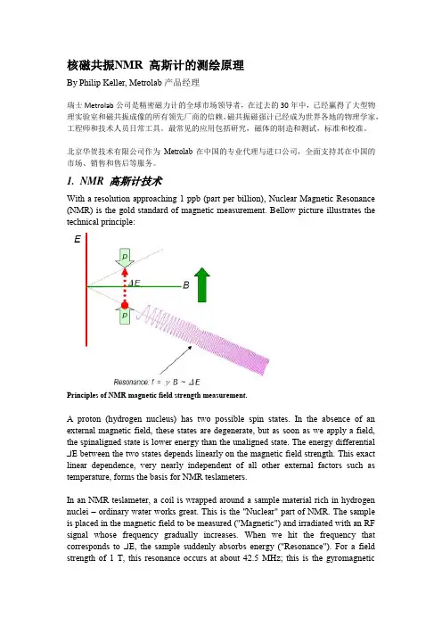
1.NMR 高斯计技术With a resolution approaching 1 ppb (part per billion), Nuclear Magnetic Resonance (NMR) is the gold standard of magnetic measurement. Bellow picture illustrates the technical principle:Principles of NMR magnetic field strength measurement.A proton (hydrogen nucleus) has two possible spin states. In the absence of an external magnetic field, these states are degenerate, but as soon as we apply a field, the spinaligned state is lower energy than the unaligned state. The energy differential ΔE between the two states depends linearly on the magnetic field strength. This exact linear dependence, very nearly independent of all other external factors such as temperature, forms the basis for NMR teslameters.In an NMR teslameter, a coil is wrapped around a sample material rich in hydrogen nuclei – ordinary water works great. This is the "Nuclear" part of NMR. The sample is placed in the magnetic field to be measured ("Magnetic") and irradiated with an RF signal whose frequency gradually increases. When we hit the frequency that corresponds to ΔE, the sample suddenly absorbs energy ("Resonance"). For a field strength of 1 T, this resonance occurs at about 42.5 MHz; this is the gyromagneticratio (γ) for hydrogen nuclei.The resonance is extremely narrow, and so the frequency provides an extremely precise measure of the magnetic field strength.NMR has some overwhelming advantages over other measurement technologies:- extremely precise;- no drift; and- measures total field.That last point is perhaps not obvious. In fact, the protons align themselves with the magnetic field, and the resonance always occurs at B/γ, regardless of how we orient our coil. It turns out, however, that the best coupling between the RF field and the proton spins is achieved when the magnetic field is perpendicular to the coil's axis. In fact, NMR has a blind spot when the coil's axis is exactly aligned with the magnetic field.NMR also has substantial limitations:- Uniform field only: In a field gradient, one edge of the sample will resonate at one frequency, and the opposite edge at another. As the gradient increases, the resonance signal becomes broader and shallower, until it can no longer be detected; this limit typically lies in the range of several hundred to several thousand ppm/cm. In some situations, gradient correction coils can improve this situation.- DC / low-AC fields only: NMR is a relatively slow measurement method, making it unsuitable for measuring rapidly varying fields. Here, we have to distinguish search mode from measurement mode: scanning through a large frequency range to find the resonance requires the field to remain stable for seconds; but once the search is completed, we can track the field and achieve measurement rates of up to about 100 measurements per second.- Low fields require a large sample, ESR or pre-polarization: As the field and, consequently, the energy gap between the spin states tends towards zero, the populations of the two states tend to become equal, and the strength of the resonance diminishes. There are three possible remedies:●Use a very large sample to increase the number of spin-flips.●oPre-polarize the sample in a strong field to populate the spin-aligned state,and then remove this bias field during the measurement.●Use ESR, i.e. the spin of orbital electrons instead of protons, because thesehave a gyromagnetic ratio (γ) three orders of magnitude higher than protons.2.NMR 核磁共振测绘To build an NMR mapper, we need:- NMR probe or probe array. As we will see in the example, a probe array ramatically speeds up the acquisition and simplifies the jig.- Positioning jig.- NMR teslameter (the electronics).The output of an NMR mapper is straightforward:- total field B,- point-sampled,In fact, the size of the "points" are determined by the size of our NMR sample, which is typically a few millimetres in diameter.- very high precision.Well below 1 ppm, in the best case approaching 1 ppb.Computational post-processing depends very much on the application. The typical postprocessing for MRI applications is described in the following section.Close-up of an NMR probe array. Each probe – one of them is circled – is mounted on itsown circuit card. Such probe arrays typically contains 24 or 32 probes (maximum 96).3.NMR核磁共振测绘–案例The most widespread use of NMR mapping relates to the development, manufacturing and installation of MRI (Magnetic Resonance Imaging) magnets. These can be permanent, resistive, or superconducting magnets, with a typical field strength between 0.2 and 7 T.Technically, the preferred shape is a torroid, but for improved access to the patient, or for a less claustrophobic feel, C-shaped magnets are sometimes used. Most modern full-body systems from the major manufacturers use superconducting torroids, 1.5 or 3 T, as illustrated in Figure 12.Example of modern full-body MRI scanner (Philips Achieva).The homogeneity of the field in the imaging region must typically be guaranteed to within a few ppm. Since minor, unavoidable manufacturing variations cause inhomogeneities generally two orders of magnitude greater than that, the homogeneity must be adjusted in a process called shimming.The overall shimming procedure is to map the field, analyze the map, adjust the field with iron shims and/or shim-coil current adjustments, and to remap the field to verify the results.If necessary, this process is repeated until the specified homogeneity is achieved. The same process, and usually the same equipment, is used in R&D, manufacturing and installation. The measurement is extremely sensitive, and obscure effects such as the passing of an overhead crane or the return current of a nearby train can cause hugeerrors.NMR mapping jigs for torroid- and C-shaped MRI magnets, respectively.The probe arrays and jigs shown in Figure 11 and Figure 13 generate a map of thetotal field on the surface of a sphere. As long as there are no currents or magneticmaterial inside this sphere, and assuming the direction of the field is known, the fieldat every point inside the sphere can be calculated from Maxwell's equations. Generally we use an expansion in spherical harmonics to perform this computation.It is worth noting that the jigs shown are much simpler that in the previous examples. Fundamentally, there are two reasons for this:- Using a probe array reduces the required motion to a single dimension.- Partly because the field is so uniform, and partly because the NMR sample points are fairly large, the requirements on the positioning precision are much less –typically 0.1mm. Compare that to the 0.1 μm for the Hall mapper example!4.问答To summarize our observations from these different examples of magnetic mapping, here is a small check-list of key questions to ask if you want (rather, need) to build a mapper:- Use: R&D, production, field service?It makes a big difference if a system is to be used once in a while for R&D, or all the time in production, or packed up in a suitcase for field service.- Measurement: field components, total field, integral, gradient?Do you really need Bx, By, Bz, or do you really need B, or an integral or gradient of B?By choosing the appropriate measurement technology, you may be able to speed up the acquisition as well improve your precision.- Field: strength, uniformity, AC/DC, stability?The characteristics of your field also play an important role in the choice of measurement technology.- Precision: 10% or 10 ppm?…as does the precision required.- Positioning: access, range, precision, reproducibility?The design of your jig is as important as the choice of magnetic sensor. What sort of access do you have to the region to be measured? What positioning precision do you need? How reproducible must the positioning be?- Environment: vacuum, cryogenic?The environment changes dramatically depending on whether you're in a lab, on a production floor or in the field. In addition, magnetic systems are often combined with vacuums and cryogenic temperatures. Hall effect sensors, for example, don't work at liquid-helium temperatures.- Speed: cost, external error sources, human error?Making a fast mapper may not cost more; for example, we saw that the simplification of the jig may more than make up for the costs of a sensor array. In addition, the improved speed dramatically reduces external and human error.。

a r X i v :a s t r o -p h /0310699v 3 13 F eb 2004The Uncertainty in Newton’s Constant and Precision Predictions of the PrimordialHelium AbundanceRobert J.ScherrerDepartment of Physics and Astronomy,Vanderbilt University,Nashville,TN37235The current uncertainty in Newton’s constant,G N ,is of the order of 0.15%.For values of the baryon to photon ratio consistent with both cosmic microwave background observations and the primordial deuterium abundance,this uncertainty in G N corresponds to an uncertainty in the primordial 4He mass fraction,Y P ,of ±1.3×10−4.This uncertainty in Y P is comparable to the effect from the current uncertainty in the neutron lifetime,τn ,which is often treated as the dominant uncertainty in calculations of Y P .Recent measurements of G N seem to be converging within a smaller range;a reduction in the estimated error on G N by a factor of 10would essentially eliminate it as a source of uncertainty the calculation of the primordial 4He abundance.Big Bang nucleosynthesis (BBN)represents one of the key successes of modern cosmology [1,2].In recent years,the BBN production of deuterium has emerged as the most useful constraint on the baryon density in the universe,both because of observations of deuterium in (presumably unprocessed)high-redshift QSO absorption line systems (see Ref.[3],and references therein),and the fact that the predicted BBN yields of deuterium are highly sensitive to the baryon density.These arguments give a baryon density parameter Ωb h 2,of [3]Ωb h 2=0.0194−0.0234,(1)which is in excellent agreement with the baryon den-sity derived by the WMAP team from recent cosmic mi-crowave background observations [4]:Ωb h 2=0.022−0.024.(2)Given these limits on the baryon density,BBN predicts the primordial abundances of 4He and 7Li.Because the 4He abundance is particularly sensitive to new physics beyond the standard model,a comparison between the predicted and observed abundances of 4He can be used to constrain,for example,neutrino degeneracy or extra relativistic degrees of freedom (see,e.g.,Refs.[5,6]).For this reason,it is useful to obtain the most accurate possible theoretical predictions for the primordial 4He mass fraction,Y P .The primordial production of 4He is controlled by the competition between the rates for the processes which govern the interconversion of neutrons and protons,n +νe ↔p +e −,n +e +↔p +¯νe ,n ↔p +e −+¯νe ,(3)and the expansion rate of the Universe,given by˙R3πG N ρ1/2.(4)In BBN calculations,the weak interaction rates are scaled offof the inverse of the neutron lifetime,τn .When these rates are faster than the expansion rate,the neutron-to-proton ratio (n/p )tracks its equilibrium value.As the Universe expands and cools,the expan-sion rate comes to dominate and n/p essentially freezes out.Nearly all the neutrons which survive this freeze-out are bound into 4He when deuterium becomes sta-ble against photodisintegration.Following the initial calculations of Wagoner,Fowler,and Hoyle [7],numer-ous groups examined higher-order corrections to the 4He production.The first such systematic attempt was un-dertaken by Dicus et al.[8],who examined the effects of Coulomb and radiative corrections to the weak rates,finite-temperature QED effects,and incomplete neutrino ter investigations included more detailed ex-amination of Coulomb and radiative corrections to the weak rates [9,10,11,12],finite-temperature QED ef-fects [13],and incomplete neutrino decoupling [14],as well as an examination of the effects of finite nuclear mass [15].These effects were systematized by Lopez and Turner [16](see also Ref.[17]),who argued that all the-oretical corrections larger than the effect of the uncer-tainty in the neutron lifetime had been accounted for,yielding a total theoretical uncertainty ∆Y P <0.0002.Assuming an uncertainty of ±2sec in the neutron life-time,the corresponding experimental uncertainty in Y P is ∆Y P =±0.0004.Similar results were obtained in Ref.[17].Two relevant changes have occurred since the publica-tion of Refs.[16,17].First,the estimated uncertainty in the neutron lifetime has decreased,with the current value being [18]τn =885.7±0.8sec .(5)Second,the estimated uncertainty in the value of G N has increased .The value currently recommended by CO-DATA (Committee on Data for Science and Technology)is [19]G N =6.673±0.010×10−8cm 3gm −1sec −2.(6)This represents a factor of twelve increase over the pre-vious recommended uncertainty [20],and is primarily due to an anomalously high value for G determined by Michaelis,Haars,and Augustin [21].(See Table 1).2Reference6.67407(22)Quinn,et al.(2001)[30]6.674215(92)Luo et al.(1999)[32]6.6742(7)Schwarz et al.(1999)[34]6.6749(14)Kleinevoss et al.(1999)[36]6.673(10)CODATA(1986)[20]3[13]A.J.Heckler,Phys.Rev.D49,611(1994).[14]S.Dodelson and M.S.Turner,Phys.Rev.D46,3372(1992).[15]R.E.Lopez,M.S.Turner,and G.Gyuk,Phys.Rev.D56,3191(1997).[16]R.E.Lopez and M.S.Turner,Phys.Rev.D59,103502(1999).[17]S.Esposito,G.Mangano,G.Miele,and O.Pisanti,Nucl.Phys.B540,3(1999).[18]K.Hagiwara,et al.,Phys.Rev.D66,010001(2002).[19]P.J.Mohr and B.N.Taylor,Rev.Mod.Phys.72,351(2000).[20]E.R.Cohen and B.N.Taylor,Rev.Mod.Phys.59,1121(1987).[21]W.Michaelis,H.Haars,and R.Augustin,Metrologia32,267(1996).[22]R.H.Cyburt,astro-ph/0401091.[23]L.M.Krauss and P.Romanelli,Ap.J.358,47(1990).[24]L.M.Krauss and P.Kernan,Phys.Lett.B347,347(1995).[25]I.P.Lopes and J.Silk,astro-ph/0112310.[26]B.Ricci and F.L.Villante,Phys.Lett.B549,20(2002).[27]O.Zahn and M.Zaldarriaga,Phys.Rev.D67,063002(2003).[28]G.T.Gillies,Meas.Sci.Technol.10,421(1999).[29]St.Schlamminger,E.Holzschuh,and W.K¨u dig,Phys.Rev.Lett.89,161102(2002).[30]T.J.Quinn,C.C.Speake,S.J.Richman,R.S.Davis,andA.Picard,Phys.Rev.Lett.87,111101(2001).[31]J.H.Gundlach and S.M.Merkowitz,Phys.Rev.Lett.85,2869(2000).[32]Luo,J.,Hu,Z.K.,Fu X.H.,Fan S.H.,and Tang,M.X.,Phys.Rev.D59,042001(1999).[33]M.P.Fitzgerald and T.R.Armstrong,Meas.Sci.Technol10,439(1999).[34]J.P.Schwarz,D.S.Robertson,T.M.Niebauer,and J.E.Faller,Meas.Sci.Technol.10,478(1999).[35]F.Nolting,J.Schurr,S.Schlamminger,and W.K¨u ndig,Meas.Sci.Technol.10,487(1999).[36]U.Kleinevoss,H.Meyer,A.Schumacher,and S.Hart-mann,Meas.Sci.Technol.10,492(1999).。

Shanxi University Atomic Physics
1.1 Introduction
The origins of atomic physics :quantum mechanics Bohr model of the H This introductory chapter surveys some of the early ideas: Spectrum of atomic H and Bohr Theory Einstein's treatment of interaction of atom with light the Zeeman effect Rutherford scattering And so on
Shanxi University Atomic Physics
1.2 Spectrum of atomic hydrogen_3
Wavenumbers may seem rather old-fashioned but they are very useful in atomic physics
the characteristic spectrum for atoms is composed of discrete lines that are the ‘fingerprint' of the element.
In 1888, the Swedish professor J. Rydberg found that the spectral lines in hydrogen obey the following mathematical formula:
Shanxi University Atomic Physics
Lyman series: n’ = 2; 3; 4; … n = 1. Balmer (n = 2), Paschen series: (n = 3), Brackett (n = 4) and Pfund (n = 5)

5 |
CAUGHEY-THOMAS MOBILITY
Solved with COMSOL ure 5: Plot of the electron drift velocity for the constant mobility case. Since the mobility does not decrease as the electric field increases, the drift velocity becomes very high.
where T is the lattice temperature, μin,n and μin,p are the electron and hole input mobilities, and Fn and Fp are the driving forces for electrons and holes (currently Fn=E||,n and Fp=E||,p where E||,n is the component of the electric field parallel to the electron current and E||,p is the component of the electric field parallel to the hole current). All other parameters in the model are material properties (note that v0,n and v0,p are the saturation velocities for electrons and holes and have units of m/s). The material properties for Silicon are also obtained from Ref. 1.

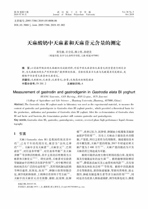
武汉轻工大学学报Journai of Wuhan Polytechnio University V c S.38Nr.5Oct.2019第38卷第5期2019年10月文章编号：2095N386(2019)05-0006-06DOI：10.3969/j.issn.2095N386.2019.05.002天麻酸奶中天麻素和天麻＜元含量的测定黄先敏，甘会廷,韩立乾,孙建美（昭通学院农学与生命科学学院，云南昭通657000）摘要:以实验所做出的天麻酸奶为试验材料，对其中的天麻素和天麻昔元的含量进行测定分析，为天麻酸奶的生产利用和推广提供理论依据。

实验结果显示天麻与乳酸菌共同发酵后，发酵物中仍含有天麻素和天麻昔元。

关键词:天麻酸奶;天麻素;天麻昔元;含量;反相高效液相色谱法中图分类号:TS201.2文献标识码：AMeasurement of gastrodin and gastrodigenin in Gastrodia elata Bl yoghurt HUANG Xian-min.,GAN Hui-ting,HAN Li-qian,SUN Jian-mei(College of Agriculturo and Life Science,Zhaotong University,Zhaotong,657000,China)Abstract：The Gastrodia elata BI yoghurt made in laboratoro was used as the experimentai materiai,O s mecsure the content of gastrodin and gastrodioenin in Gastrodia elata BI yoghui powdco,which provided a theoreticoi basis fof the production,utilization and promotion of Gastrodia elata BI yorhuri.AOs the co-femientation of Gastrodia elata BI and lactic acid bacteaa,tar femientation product stili contains gastrodin and gastrodiaenia.Key words:Gastrodia elata BI%gastrodin%gastrodiaenin%content%reversed phass high perfomianco liquia chroma-iogoaphy1引言天麻（Gastuodia elatr BI）是我国传统名贵中药［1］，已有千年的药用历史，被誉为“治风之神药”&2-'（天麻中含有天麻素⑷、天麻昔元［5］、巴利森昔&6'、对k基苯甲醛切、对k基苯甲酸［8'及天麻多糖［9］等多种活性物质，其中主要的活性物质为天麻素和天麻昔元&10N1'。

湍流长度尺度英文Turbulence Length ScalesTurbulence is a complex and fascinating phenomenon that has been the subject of extensive research and study in the field of fluid mechanics. One of the key aspects of turbulence is the concept of turbulence length scales, which refers to the range of different-sized eddies or vortices that are present in a turbulent flow. These length scales play a crucial role in understanding and predicting the behavior of turbulent flows, and they have important implications in a wide range of engineering and scientific applications.The smallest length scale in a turbulent flow is known as the Kolmogorov length scale, named after the Russian mathematician and physicist Andrey Kolmogorov. This length scale represents the size of the smallest eddies or vortices in the flow, and it is determined by the rate of energy dissipation and the kinematic viscosity of the fluid. The Kolmogorov length scale is typically denoted by the Greek letter η (eta) and can be expressed as η = (ν^3/ε)^(1/4), where ν is the kinematic viscosity of the fluid and ε is the rate of energy dissipation.The Kolmogorov length scale is important because it represents the scale at which viscous forces become dominant and energy is dissipated into heat. Below this length scale, the flow is considered to be in the dissipation range, where the eddies are too small to sustain their own motion and are rapidly broken down by viscous forces. The Kolmogorov length scale is therefore a critical parameter in the study of turbulence, as it helps to define the range of scales over which energy is transferred and dissipated within the flow.Another important length scale in turbulence is the integral length scale, which represents the size of the largest eddies or vortices in the flow. The integral length scale is typically denoted by the symbol L and is a measure of the size of the energy-containing eddies, which are responsible for the bulk of the turbulent kinetic energy in the flow. The integral length scale is often determined by the geometry of the flow domain or the boundary conditions, and it can be used to estimate the overall scale of the turbulent motion.Between the Kolmogorov length scale and the integral length scale, there is a range of intermediate length scales known as the inertial subrange. This range is characterized by the presence of eddies that are large enough to be unaffected by viscous forces, but small enough to be unaffected by the large-scale features of the flow. In this inertial subrange, the energy is transferred from the large eddies to the smaller eddies through a process known as the energycascade, where energy is transferred from larger scales to smaller scales without significant dissipation.The energy cascade is a fundamental concept in turbulence theory and is described by Kolmogorov's famous 1941 theory, which predicts that the energy spectrum in the inertial subrange should follow a power law with a slope of -5/3. This power law relationship has been extensively verified through experimental and numerical studies, and it has important implications for the modeling and prediction of turbulent flows.In addition to the Kolmogorov and integral length scales, there are other important length scales in turbulence that are relevant to specific applications or flow regimes. For example, in wall-bounded flows, the viscous length scale and the boundary layer thickness are important parameters that can influence the turbulent structure and behavior. In compressible flows, the Taylor microscale and the Corrsin scale are also relevant length scales that can provide insight into the characteristics of the turbulence.The understanding of turbulence length scales is crucial for a wide range of engineering and scientific applications, including fluid dynamics, aerodynamics, meteorology, oceanography, and astrophysics. By understanding the different length scales and their relationships, researchers and engineers can better predict andmodel the behavior of turbulent flows, leading to improved designs, more accurate simulations, and a deeper understanding of the fundamental principles of fluid mechanics.In conclusion, turbulence length scales are a fundamental concept in the study of turbulent flows, and they play a crucial role in our understanding and modeling of this complex and fascinating phenomenon. From the Kolmogorov length scale to the integral length scale and the inertial subrange, these length scales provide valuable insights into the structure and dynamics of turbulence, and they continue to be an active area of research and exploration in the field of fluid mechanics.。

由 （ 式可得：Ｉ 【 ０由于 Ｄ是对角矩 ３ ） ＝ 阵， ， 因此 至少有一对角元 素为 ０ 。 因为 Ｕ＝ ＵＬ Ｄ Ｄ ，ＶＬ 设该潮流计算 是 ｎ 节点 系统 。 所以（ ） ２） ２ 或（ 工 ａ ｂ弋有一个成立 ， Ｕ 中有一 Ｈ子矩阵奇异 ，那 么 Ｈ矩阵各 个列向量线 性相 即 ｎ 一１ 零行 或 中有一零列 。 ｕ 中行为零 ， 是行相关 隋况 ；丰中列 为 关 ， ： 这 Ｌ 即 － ＝ （ 不全为 ０ ｑ ０ ） 零， 这是列相关 隋况。 其 中： 是 Ｈ矩 阵的列 向量 ，１是相关 系 ｃ Ｔ Ａ矩 阵奇异 ， 那么 Ａ矩 阵行 向量 、 向量线 列 数 。由潮流雅可 比矩阵元素计算可知 ： 性相关 ， 即： 对 同一节点 ， 素和 Ｊ 素的计 算具 有完 Ｈ元 元 全相似 的表达式 ，因此 ，矩 阵的各个列 向量也 Ｊ （ａ ４） 应满足（ ， 即：
中国新技术新产 品
一７
！
Ｃ ｉａ Ｎ ｗ Ｔ ｃ ｎ ｌ ｇｅ ｎ ｒ ｄ ｃｓ ｈ ｎ ｅ ｅ ｈ ｏｏ ｉｓａ ｄ Ｐ ｏ ｕ ｔ
高 新 技 术
新型停 水 自动关 闭阀结构 、 点及操作要 点 特
张金龙 曹 艳
（ 西安航 空技 术高等专科学校机械 工程 系， 陕西 西安 ７ ０ ７ ） １０ ７
中图分 类 号 ： ４ ． 文献标 识 码 ： Ｇ６ ４５ Ａ
。
Ｉ 言 。在 日常生 活 中 ， 前 由于停 水时 忘记 关 闭 阀门 ， 水 时 也没 能及 时 关 闭 阀门 ， 来 造成 水 资源 浪 费甚 至形 成安 全 隐 患 的情况 屡 见不 鲜 。 着全 民节 水 概念 不 断深入 人 心 ， 一 问 随 这 题 引起 各方 关 注 。 因此 急 需设 计 一 款可 以在 停 水 时 自动关 闭 的水 阀 ，它 能够 在停 水 后 即 使 人们 忘记 关 闭 水 龙 头 也 能实 现 自动 关 闭 ， 而再 次 来水 时 不 至于 出 现水 患 的情 况 ，能够 有 效 的节 约水 资源 。 要 实 现 自动 关 闭 功 能首 先 要 有 动 力 ， 这 方 面可 以借 助 磁性 元件 的磁 力 、弹性 元 件 的 弹力 、 力 等外 力 ， 时考 虑供 水 和停 水 时 的 重 同 水 压变 化 ， 通过 联 动机 构实 现 。 ２停 水 自动关 闭 阀 的结 构 及 特点 。利用 水 压 、 力 等 力 学 特 性 ， 过 一 系 列 的实 验 、 重 经 改 进 ， 发 出一 种 简单 、 行 的带 有 停水 自锁 研 可 机 构 的水 阀 。 款 水 阀为纯 机 械构 造 ， 阀体 这 以 为 主体 框 架 ， 有 阀 芯 、 封 圈 、 心 轮 以及 配 密 偏 手柄 ， 无弹 性元 件 ， 作状 况 不 受环 境 和时 间 工 的 限制 ， 构 简 单 ， 价 低 廉 并 方 便拆 换 ， 结 造 整 体 可靠 性 高 。 停 水 自动关 闭 阀结 构 原 理 如 图 １ 示 ， 所 实 物 如 图 ２所示 。序号 ｌ 水 阀 的偏 心轮 ， 为 ２ 为 ０ 型密 封 圈 ， 为 Ｖ型 密封 圈 ， 阀体 ， ３ ４为 ５ 为 阀芯 ， 销 轴 ， 手 柄 。 阀体 ４是 主 框 ６为 ７为 架 ， 来装 配其 它 元 件 ， 进 水 口和 出 水 口； 用 有 阀芯 ５的顶 端 与末 端分 别 装有 Ｖ 型密 封 圈 ３ 和 ０ 型 密 封 圈 ２ｖ 型 密 封 圈 ３利 用 其 锥 面 ， 与 阀体 ４内部 锥 面 配合 实 现 停 水 时 密 封 ， 而 ０型密 封 圈 ２与 阀体 ４内壁 的接 触 实 现来 水 时对 水 阀末 端 的密 封 ，在 阀 芯 ５的 中部 开两

Published online July 30, 2008. Transmitted by Assoc. Editor P. M. Adler.
hydraulic property such as permeability can be found. Recently, the LBM coupled with the visualization computing technique and digital image ͓8,9,67–71͔ is used to simulate the flow and transport in real porous media. However, the accuracy of the LBM has often been debated ͓52,74͔ since its emerging. In addition, the results from the LBM and other numerical simulations as well as experimental measurements are usually correlated as curves or correlations with one or more empirical constants, and the mechanisms behind these constants are often ignored. In order to get a better understanding of the mechanisms for flow in porous media, the analytical solution for flow and transport properties in porous media is desirable and becomes a challenging task. Pores in real porous media can be very large ͑in the order of meters͒ or very small ͑in the order of nanometers͒, and they may be three dimensional and some of them are connected. Pores may be formed due to physical and chemical reactions. The shapes of pores are usually quite different depending on materials such as stainless screen, packed beds of particles, chips in computers and mobiles, polyurethane foam, fibrous preforms, gas diffusion layer in fuel cells, sandstone in oil/water reservoirs and soils, etc. Despite extreme complexity of real porous media, an equivalent macroscopic model is possible on the condition that there exists a separation of scales between the heterogeneity characteristic length and a macroscopic characteristic length related to the macroscopically investigated sample and/or the physical phenomenon at the macroscopic scale. The fractal porous media may satisfy this condition and the macroscopic transport properties in the media can thus be studied by the fractal geometry theory. It has been shown that fractal geometry ͓75͔ may have the potential in analysis of flow and transport properties in porous media. Katz and Thompson ͓76͔ might be the first to present the experimental evidence indicating that the pore spaces of a set of porous sandstone samples are fractals and are self-similar over three to four orders of magnitude in length extending from 10 Å to 100 ␮m. They argued that the pore volume is a fractal with the same fractal dimension as the pore-rock interface. This conclusion was supported by correctly predicting the porosity from the fractal dimension, which was measured by a log-log plot of a number of pores versus the pore size, and a fractal correlation was obtained as SEPTEMBER 2008, Vol. 61 / 050801-1

Louis Pasteur Some of his works are: separation of mirror image molecules and effect of polarized light identification of the parasite that was killing silkworms James Maxwell He is known for the "Treatise on Electricity and Magnetism" published in 1873. Maxwell independently developed the "Maxwell-Boltzmann kinetic theory of gases". Edwin Hubble "Hubble's Law" stated that galaxies move away from each other at a speed determined by the distance that separated them. He classified galaxies as per their distance, shape, brightness patterns and content. Paul Dirac He received a Nobel prize in 1933 for the work on antiparticles. The "Dirac equation" was a version of the Schrodinger's equation.
Barbara Goldsmith is a noted author, historian. Her best-selling books include The Straw Man, Little Gloria…Happy at Last, Johnson v. Johnson, and Other Powers: The Age of Suffrage, Spiritualism, and the Scandalous Victoria Woodhull (soon to be a major motion picture produced by Kathleen Kennedy for Universal Studios) and Obsessive Genius: The Inner World of Marie Curie. Barbara Goldsmith has long been at the forefront of the effort to preserve our written heritage. She is the donor of the Goldsmith Conservation and Preservation Laboratories at the New Yse Divisions were recently named in her honor.

单矢量水听器水中多目标方位跟踪方法张维;尚玲【摘要】The direction of arrival (DOA) of multiple targets was acquired by solving non-liner correlation equations involving acoustic pressure and particle velocity with quantum particle swarm algorithm.In order to improve the precision, the DOA tracks of multiple targets were fitted with the method of least squares, the prediction model was found and then the DOA tracks were optimized by Kalman filter.The results indicate that the DOA of multiple targets can be resolved with the single vector hydrophone and the results should be expressed by statistic characteristics.The maximum number of unknown sources is 7.As the number increases, the DOA error is more serious.When the signal to noise ratio is higher, the resolution ratio and precision are also higher and the deviation is smaller.More importantly, the precision of DOA can be improved effectively by the method of data fitting and the Kalman filter.%采用量子粒子群求解声压和质点振速组成的非线性相关方程组,实现多目标声源方位的估计.为提高精度,应用最小二乘法对测量结果进行拟合并建立预测模型,通过卡尔曼滤波对方位轨迹进行优化.结果表明:单矢量水听器能够同时分辨多个目标方位,解算结果应使用统计特性表示;采用本方法最多能分辨7个目标,目标个数越多,方位误差越大;信噪比越高,分辨率和精度越高,偏差越小;通过数据拟合然后卡尔曼滤波的方法能够有效提高目标方位跟踪精度.【期刊名称】《国防科技大学学报》【年(卷),期】2017(039)002【总页数】6页(P114-119)【关键词】多目标方位;单矢量水听器;卡尔曼滤波;最小二乘法;量子粒子群【作者】张维;尚玲【作者单位】中国船舶重工集团公司第七一〇研究所, 湖北宜昌 443003;中国船舶重工集团公司第七一〇研究所, 湖北宜昌 443003【正文语种】中文【中图分类】TN911.7单个矢量水听器能同时拾取声压和质点振速信息，在各向同性噪声背景中，采用平均声强器[1-2]、最大似然检测[3-4]、互谱法[5]就可以对目标进行定向。

a r X i v :h e p -e x /9901006v 1 8 J a n 1999SLAC-PUB-7983Jan.1999Measurement of the Proton and Deuteron Spin Structure Functions g 2andAsymmetry A 2∗The E155CollaborationP.L.Anthony,16R.G.Arnold,1T.Averett,5,††H.R.Band,21M.C.Berisso,12H.Borel,7P.E.Bosted,1S.L.B¨u ltmann,19M.Buenerd,16,†T.Chupp,13S.Churchwell,12,‡G.R.Court,10D.Crabb,19D.Day,19P.Decowski,15P.DePietro,1R.Erbacher,16,17R.Erickson,16A.Feltham,19H.Fonvieille,3E.Frlez,19R.Gearhart,16V.Ghazikhanian,6J.Gomez,18K.A.Griffioen,20C.Harris,19M.A.Houlden,10E.W.Hughes,5C.E.Hyde-Wright,14G.Igo,6S.Incerti,3J.Jensen,5J.K.Johnson,21P.M.King,20Yu.G.Kolomensky,5,12S.E.Kuhn,14R.Lindgren,19R.M.Lombard-Nelsen,7J.Marroncle,7J.McCarthy,19P.McKee,19W.Meyer,4G.S.Mitchell,21J.Mitchell,18M.Olson,9,§§S.Penttila,11G.A.Peterson,12G.G.Petratos,9R.Pitthan,16D.Pocanic,19R.Prepost,21C.Prescott,16L.M.Qin,14B.A.Raue,8D.Reyna,1,♥L.S.Rochester,16S.Rock,1O.Rondon-Aramayo,19F.Sabatie,7I.Sick,2T.Smith,13L.Sorrell,1F.Staley,7S.St.Lorant,16L.M.Stuart,16,§Z.Szalata,1Y.Terrien,7A.Tobias,19L.Todor,14T.Toole,1S.Trentalange,6D.Walz,16R.C.Welsh,13F.R.Wesselmann,14T.R.Wright,21C.C.Young,16M.Zeier,2H.Zhu,19B.Zihlmann 191American University,Washington,D.C.200162Institut f¨u r Physik der Universit¨a t Basel,CH-40=56Basel,Switzerland 3University Blaise Pascal,LPC IN2P3/CNRS F-63170Aubiere Cedex,Fran=ce4Ruhr-Universit¨a t Bochum,Universit¨a tstr.150,=20Bochum,Germany 5California Institute of Technology,Pasadena,California 911256University of California,Los Angeles,California 900957DAPNIA-Service de Physique Nucleaire,CEA-Saclay,F-91191Gif/Yvette Cedex,France8Florida International University,Miami,Florida 33199.9Kent State University,Kent,Ohio 4424210University of Liverpool,Liverpool L693BX,United Kingdom 11Los Alamos National Laboratory,Los Alamos,New Mexico 8754512University of Massachusetts,Amherst,Massachusetts 0100313University of Michigan,Ann Arbor,Michigan 4810914Old Dominion University,Norfolk,Virginia 2352915Smith College,Northampton,Massachusetts 0106316Stanford Linear Accelerator Center,Stanford,California 9430917Stanford University,Stanford,California9430518Thomas Jefferson National Accelerator Facility,Newport News,Virginia23606 19University of Virginia,Charlottesville,Virginia22901 20The College of William and Mary,Williamsburg,Virginia2318721University of Wisconsin,Madison,Wisconsin53706AbstractWe have measured the spin structure functions g p2and g d2and the virtual photon asymmetries A p2and A d2over the kinematic range0.02≤x≤0.8and1.0≤Q2≤30(GeV/c)2by scattering38.8GeV longitudinally polarized electrons from transversely polarized NH3and6LiD targets.The absolute value of A2√is significantly smaller than theThe deep inelastic spin structure functions of the nucleons,g 1and g 2,depend on the spin distribution of the partons and their correlations.The function g 1can be primarily understood in terms of the quark parton model (QPM)and perturbative QCD with higher twist terms at low Q 2.There exists nosuchpicturefor g 2.Feynman[1]claimed that the transverse structure function g T =g 1+g 2had a simple parton interpretation in terms of the transverse polarization of the quark spins which is proportional to quark masses.However,g 2is sensitive to higher twist effects such as quark-gluon correlations[2]and is not easily interpreted in pQCD where such effects are not included.By interpreting g 2using the operator product expansion (OPE)[2,3],it is possible to study contributions to the nucleon spin structure beyond the simple QPM.The virtual photon-nucleon asymmetry A 2is proportional to g T /F 2where F 2is the unpolarized structure function.The structure function g 2can be written [4]:g 2(x,Q 2)=g W W2(x,Q 2)+ydy.∂ymywhere x is the Bjorken scaling variable and Q 2is the absolute value of the virtual photonfour-momentum squared.The twist-2term g W W2was derived by Wandzura and Wilczek [5]and depends only on the well-measured g 1[6,7,8,9,10,11].The function h T (x,Q 2)is an additional twist-2contribution [12,4]that depends on the transverse polarization density in the nucleon.The h T contribution to2+O (M 2/Q 2),n =0,2,4,...1x n g 2(x,Q 2)dx =n2+O (M 2/Q 2),n =2,4,...(2)In these integrals the contribution of d n is not suppressed relative to the twist-2contribution and thus can be easily extracted.Neglecting (1/Q )terms,the d n matrix elements can be written as:d n =2(n +1)g 2(x,Q 2)dx (3)and thus measures deviations of g2from the twist-2g W Wterm.2The Burkhardt-Cottingham sum rule[14]for g2at large Q2,10g2(x)dx=0,(4)was derived from virtual Compton scattering dispersion relations.It does not follow from the OPE since the n=0sum rule is not defined for g2.Its validity depends on the lack of singularities for g2at x=0.The Efremov-Leader-Teryaev(ELT)sum rule[15]involves the valence quark contributions to g1and g2:10x[g V1(x)+2g V2(x)]dx=0.(5)Assuming that the sea quarks are the same in protons and neutrons the sum rule takes a form 10x[g p1(x)+2g p2(x)−g n1(x)−2g n2(x)]dx=0that we can apply to our data.Measurements of g2and A2exist for the proton and deuteron[7,16,17,18],as well as for the neutron[8,19].In this Letter,we report new measurements of g2and A2for the proton and deuteron made during experiment E155at SLAC.A38.80GeV,120Hz electron beam with a longitudinal polarization of(81.3±2.0)% struck transversely polarized NH3[7]or6LiD[20]targets.The beam helicity direction was randomly chosen pulse-by-pulse.Scattered electrons were detected in three independent spectrometers centered at2.75◦,5.5◦,and10.5o.The two small angle spectrometers were the same as in SLAC E154[9],while the large angle spectrometer was new for this experiment. It consisted of a single dipole magnet and two quadrupoles,and covered a momentum range from7to20GeV,and scattering angle range from9.6◦to12.5◦with a maximum solid angle of1.5msr at8GeV.Electrons were separated from a much largerflux of pions using a gas ˇCerenkov counter and a segmented electromagnetic calorimeter.Further information on the technique can be found in references[7,9,10].The measured counting rate asymmetries from the two beam helicities were corrected for beam polarization,target polarization,tracking efficiencies,pion and charge symmetric backgrounds,and radiative effects.Uncertainties in the radiative corrections were estimated by varying the input models over a range consistent with the measured data.The deuteron data were extracted from the6LiD results by applying a correction for both the lithium and deuterium nuclear wave functions with6Li∼α+d[20].The structure function g2(x,Q2) and the virtual photon absorption asymmetry A2(x,Q2)are usually determined from the two measurable asymmetries,A⊥(E,x,Q2)(dominant contribution)and A (E,x,Q2)(small contribution),corresponding to transverse and longitudinal target polarization with respect to the incoming electron beam helicity.Because in this experiment these asymmetries were measured at two different beam energies(38.8and48.3GeV respectively),we instead chose to determine g2and A2(x,Q2)from A⊥(dominant contribution)and A1(small contribution) using:F2(x,Q2)g2(x,Q2)=whereζ=η(1+ǫ)/(2ǫ),η=ǫ√Q2,d=(1−E′ǫ/E)R positivity limit and data from previous experiments.The data are in good agreement with the previous measurements and improve the accuracy for the deuteron.The combined results are significantly smaller than the positivity limit over most of the measuredrange.A2is consistent with A W W2calculated from g W W2and A p2is significantly larger thanzero around x∼0.2.Results for x g2are shown in Fig.3along with the twist-2component,x g W W2calculated using our new parameterization of the A1data.The combined SLAC dataagrees with g W W2with aχ2/(dof)of1.3and0.9for proton and deuterium respectively for 17degrees of freedom.The comparison with g2=0has similar agreement withχ2/(dof) of1.5and0.9respectively.Also shown is the bag model calculation of Stratmann[23].A recent Chiral Soliton Model calculation[24](not shown)also agrees with the data We used Eq.3to calculate the matrix elements d n assuming thatg2∝(1−x)m where m=2or3,normalized to the data for x≥0.5.Becauseg2is independent of Q2and thus thatall the Q2dependence of g2is in g W W2.The results for the proton and deuteron are-0.022±0.071and0.023±0.044respectively.Averaging with the E143results which cover a slightly more restrictive x range gives-0.015±0.026and0.010±0.039.All of these integrals are consistent with the Burkhardt-Cottingham sum rule prediction of zero.However,this does not represent a conclusive test of the sum rule because the behavior of g2as x→0is notknown.We evaluated the ELT integral,Eq.5,using our data in the measured region.The result at Q2=5(GeV/c)2is-0.015±0.036,which is consistant with the expected value of zero.Including the E143g2data[7]improves the accuracy to0.003±0.022.Again the extrapolation to x=0is not known,but in this case the contribution is suppressed by a factor of x.In summary,we have presented a new measurement of A2and g2for the proton and deuteron in the kinematic range0.02≤x≤0.8and1.0≤Q2≤30(GeV/c)2.Our results√for A2are significantly smaller than the[6]SMC collaboration:B.Adeva et al.,Phys.Lett.B302(1993)533;D.Adams et al.,Phys.Lett.B329(1994)399;B.Adeva et al.,Phys.Lett.B357(1995)248.[7]E143Collaboration:K.Abe et al.,Phys.Rev.Lett.74,346(1995);Phys.Rev.Lett.75,25(1995);Phys.Rev.D58,112003(1998).[8]E142collaboration:P.Anthony et al.,Phys.Rev.Lett.71,959(1993);Phys.Rev.D54(1996)6620.[9]E154collaboration:K.Abe et al.,Phys.Rev.Lett.79,26(1997),[10]E155collaboration:P.Anthony et al.,SLAC-PUB-7994,to be submitted to Phys.Rev.Lett.[11]HERMES collaboration:K.Ackerstaffet al.Phys.Lett.B404,383(1997); A.Airapetian et al.,hep-ex/9807015.[12]X.Song,Phys.Rev.D54(1996)1955.[13]R.G.Roberts and G.G.Ross,Phys.Lett.B373,235(1996).[14]H.Burkhardt and W.N.Cottingham,Ann.Phys.56,453(1970).[15]A.V.Efremov,O.V.Teryaev and E.Leader,Phys.Rev.D55,4307(1997).[16]SMC collaboration:D.Adams et al.,Phys.Lett.B336125(1994).[17]E143collaboration:K.Abe et al.,Phys.Rev.Lett.76,587(1996).[18]SMC collaboration:D.Adams et al.,Phys.Lett.B396338(1997).[19]E154collaboration:K.Abe et al.,Phys.Lett.B404,377(1997).[20]S.B¨u ltmann et al.,SLAC-PUB-7904(1998),Submitted to Nucl.Inst.Meth.A.[21]NMC collaboration:M.Arneodo et al.,Phys.Lett.B364,107(1995).[22]E143collaboration:K.Abe et al.,hep-ex/9808028,SLAC-PUB7927.[23]M.Stratmann,Z.Phys.C60(1993)763.[24]H.Weigel,L.Gamberg,and H.Reinhart,Phys.Rev.D55,6910(1997).[25]X.Ji and P.Unrau,Phys.Lett.B333(1994)228.[26]E.Stein et al.,Phys.Lett.B343(1995)369.[27]I.Balitsky,V.Braun and A.Kolesnichenko,Phys.Lett.B242(1990)245;B318(1993)648(Erratum).[28]B.Ehrnsperger and A.Schafer,Phys.Rev.D52,2709(1995).[29]M.G¨o ckeler et al.,Phys.Rev.D53(1996)2317.Table1:Results for A2and xg2with statistical errors for proton and deuteron at the measured x and Q2[(GeV/c)2]for the three spectrometers with E=38.8GeV.x<Q2>A p2xg p2A d2xg d20.022 1.150.149±0.1110.439±0.335−0.036±0.074−0.103±0.2120.026 1.32−0.020±0.032−0.069±0.0880.023±0.0210.060±0.0560.039 1.56−0.034±0.025−0.090±0.0570.023±0.0170.043±0.0350.062 1.940.025±0.0330.024±0.0540.012±0.0210.013±0.0340.099 2.340.016±0.046−0.020±0.0540.040±0.0310.041±0.0340.159 2.710.033±0.069−0.021±0.0560.061±0.0470.024±0.0350.255 3.010.075±0.107−0.008±0.056−0.108±0.076−0.077±0.0350.411 3.25−0.004±0.212−0.049±0.0560.273±0.1660.032±0.0360.621 3.37−0.842±0.594−0.123±0.0540.501±0.5030.019±0.0350.796 3.42−0.294±1.734−0.019±0.042−2.329±1.460−0.043±0.0240.072 3.680.185±0.1770.367±0.370−0.177±0.117−0.353±0.2310.104 4.84−0.041±0.037−0.102±0.0640.034±0.0240.050±0.0400.161 6.260.019±0.032−0.022±0.0420.007±0.022−0.007±0.0270.2567.760.098±0.0440.030±0.0390.048±0.0330.018±0.0250.4179.20−0.004±0.079−0.059±0.034−0.030±0.063−0.032±0.0220.62510.230.021±0.211−0.027±0.026−0.011±0.186−0.015±0.0170.82810.76−0.298±0.701−0.010±0.0141.102±0.6030.012±0.0080.1689.770.034±0.0710.011±0.115−0.069±0.049−0.118±0.0700.25813.700.049±0.061−0.001±0.0700.006±0.044−0.016±0.0430.43220.060.100±0.0820.006±0.0450.016±0.068−0.013±0.0290.64325.460.186±0.1360.005±0.0200.357±0.1330.030±0.0150.84129.250.670±0.3090.008±0.006−0.295±0.322−0.006±0.0040.022 1.150.149±0.1110.439±0.335−0.036±0.074−0.103±0.2120.026 1.32−0.020±0.032−0.069±0.0880.023±0.0210.060±0.0560.039 1.56−0.034±0.025−0.090±0.0570.023±0.0170.043±0.0350.062 1.990.030±0.0320.032±0.0540.006±0.0210.004±0.0330.101 3.45−0.018±0.029−0.056±0.0420.037±0.0190.045±0.0260.161 5.410.026±0.027−0.019±0.0330.006±0.019−0.007±0.0200.2567.540.084±0.0340.015±0.0290.020±0.025−0.014±0.0180.42111.750.045±0.055−0.039±0.0240.014±0.045−0.013±0.0150.63719.620.103±0.112−0.023±0.0150.246±0.1060.009±0.0100.83927.180.491±0.2790.002±0.005−0.071±0.279−0.004±0.004–0.4–0.2–0.100.100.10A 25Q 2 (GeV/c)2)11–98 8451A11015205101520Figure 1:A 2for the proton and deuteron as a function of Q 2for selected values of x.Data are for this experiment (solid)and E143[7](open).The errors are statistical;the systematic errors are negligible.The Bag Model calculation of Stratmann[23]is also shown.X0.01 A 2A 2–0.111–98 8451A20.1 1 0.20.20.40.4–0.2Figure 2:The asymmetries A 2for proton and deuteron for this experiment (E155)with data from all spectrometers averaged (Table 1).The errors are statistical;the systematicerrors are negligible.Also shown are the data from SLAC E143[7]and SMC[6].Our A W W2calculation is shown as the solid line and the√X 0.6 0.8 1.00.4 0.2 0 xg 2xg 20.10.2–0.1–0.111–988451A30.10.2Figure 3:The structure function x g 2for all spectrometers combined and data from E143[7].The errors are statistical;the systematic errors are negligible.Also shown is our twist-2g W W 2at the average Q 2of this experiment at each value of x and the calculations of Stratmann[23]and Song [12].Predictions and Datad 2d 2–0.02–0.041–998438A7–0.02–0.04–0.060.0200.02Figure 4:The twist-3matrix element d 2for the proton and deuteron from the combined data from SLAC experiments E142[8],E143[7],E154[19]and E155(Data).Also shown are theoretical models from left to right:Bag Models[12,23,25],QCD Sum Rules [26,27,28],lattice QCD [29],and Chiral Soliton Model [24].The shaded region indicates the experimental errors.。

"Hydrogen: Properties and Applications (International English Resources)"Hydrogen, the most abundant element in the universe, holds a unique position due to its various properties and wide range of applications. Below is an exploration of hydrogen's characteristics and its uses, as gathered from international English resources.Properties of Hydrogen1. Elemental Composition: Hydrogen is the lightest and simplest element, with an atomic number of 1, consisting of one proton and one electron.2. Physical State: At standard temperature and pressure, hydrogen is a colorless, odorless, and tasteless gas. It remains in a gaseous state in the Earth's atmosphere.3. Density: Hydrogen is less dense than air, making it lighter than helium and all other gases.4. Solubility: Hydrogen is slightly soluble in water and can form hydrogen hydrates under high pressure.6. Isotopes: Hydrogen has three naturally occurring isotopes: protium (no neutrons), deuterium (one neutron), and tritium (two neutrons).Applications of Hydrogen1. Energy Source: Hydrogen is widely used as a fuel in fuel cells, which generate electricity through a chemical reaction with oxygen, producing only water as a product.2. Industrial Processes: Hydrogen is crucial in various industrial processes, including the production of ammonia for fertilizers, the refining of petroleum, and the manufacture of metals.4. Energy Storage: Hydrogen can be used as an energy storage medium, particularly in conjunction with renewable energy sources like wind and solar power.5. Chemical Industry: Hydrogen is a key reactant in the production of numerous chemicals, including methanol, hydrochloric acid, and hydrogen peroxide.6. Medical Applications: Hydrogen is used in the production of contrast agents for magnetic resonance imaging (MRI) and in the treatment of certain medical conditions.This overview of hydrogen's properties and applications, based on international English resources, highlights the element's versatility and potential in various sectors. As research and technology advance, hydrogen's role in a sustainable future continues to grow."Hydrogen: Properties and Applications (International English Resources)"Continued8. Power Generation: Beyond fuel cells, hydrogen can be used in gas turbines for electricity generation, providing a cleaner alternative to fossil fuels.9. Residential Uses: Hydrogen is being explored for residential applications, such as heating and cooking, where it can replace natural gas, reducing carbon emissions.10. Green Hydrogen: The production of "green hydrogen" through electrolysis using renewable energy sources is gaining momentum, aiming to create a carbonfree energy carrier.11. Semiconductor Industry: Hydrogen is used in the semiconductor industry for cleaning and reducing processes, ensuring the purity of silicon wafers.12. Food Industry: Hydrogen is used in the production of edible oils through a process called hydrogenation, which helps to increase the shelf life and stability of fats.13. Welding and Metalworking: Hydrogen is used as a shielding gas in welding to protect the weld area from atmospheric contamination, leading to cleaner and stronger welds.14. Balloons and Airships: Due to its low density, hydrogen (or its safer alternative, helium) is used to fill balloons and airships, providing lift for aerial observation and research.15. Climate Research: Hydrogen isotopes, particularly deuterium and tritium, are used in climate studies to understand the water cycle and past climate conditions.16. Nanotechnology: Hydrogen is used in the production of hydrogenated fullerenes, which have potential applications in nanotechnology, including drug delivery systems.17. Cryogenics: Liquid hydrogen is used in cryogenic applications due to its extremely low boiling point, which is vital for cooling superconducting magnets and otherscientific equipment.18. Aeronautics: Hydrogen is being researched for potential use in hypersonic aircraft, where it could serve asa fuel for propulsion systems operating at high speeds.19. Art Preservation: Hydrogen is used in conservation processes to remove tarnish from silver and other metals without damaging the underlying surface.The diverse applications of hydrogen, as outlined in international English resources, underscore its pivotal role across multiple sectors. As the world moves towards more sustainable and ecofriendly solutions, the potential for hydrogen in both existing and emerging fields continues to expand, making it a focal point for innovation and development."Hydrogen: Properties and Applications (International English Resources)"Continued21. Biomedical Research: Hydrogen's potential as a therapeutic agent is being explored in biomedical research, including its possible role in reducing oxidative stress and inflammation in the body.23. Artillery Propulsion: Hydrogen is used in certain types of artillery, such as the HIMARS system, where it provides a highenergy, lowsmoke propellant for rocket motors.24. Metallurgical Processes: Hydrogen is essential in the production of certain metals, like titanium and stainless steel, where it is used to reduce metal oxides in therefining process.25. Semiconductor Cleaning: In the electronics industry, hydrogen is used in plasma cleaning processes to remove organic contaminants from semiconductor surfaces.27. Underwater Vehicles: Hydrogen fuel cells are being tested for use in underwater vehicles, providing a quiet and efficient power source for extended operations.28. Hydrogen Infrastructure: The development of hydrogen refueling stations and pipelines is a growing field, aiming to support the expanding hydrogen economy.29. Carbon Capture and Storage: Hydrogen can be used in processes that capture carbon dioxide from industrial emissions, helping to mitigate climate change storing or utilizing the captured CO2.30. Advanced Materials: Research into hydrogen storage materials, such as metalorganic frameworks (MOFs), is advancing, which is critical for the practical application of hydrogen as a fuel.31. Jewelry Making: Hydrogen is used in the jewelry industry for processes like hydrogen reduction, which can improve the appearance and quality of precious metals.32. Breathable Air: In closed environments like submarines and space stations, hydrogen is part of the process to regenerate breathable air removing carbon dioxide.33. Quantum Sensors: Hydrogen atoms are used in quantum sensors for highprecision measurements, which can have applications in navigation, geodesy, and fundamental physics research.35. Education and Outreach: Hydrogen is a key topic in educational programs aimed at promoting understanding of sustainable energy and the role of chemistry in modern society.。

最新完整托福模拟题阅读(一)Questions 12-20 The elements other than hydrogen and helium exist In such small quantities that it is accurate to say that the universe somewhat more than 25 percent helium by weight and somewhat less than 25 percent hydrogen. Astronomers h Questions 12-20The elements other than hydrogen and helium exist In such small quantities that it is accurate to say that the universe somewhat more than 25 percent helium by weight and somewhat less than 25 percent hydrogen.Astronomers have measured the abundance of helium throughout our galaxy and in other galaxies as well. Helium has been found In old stars, in relatively young ones, in interstellar gas, and in the distant objects known as quasars. Helium nuclei have also been found to be constituents of cosmic rays that fall on the earth (cosmic "rays" are not really a form of radiation; they consist of rapidly moving particles of numerous different kinds). It doesn't seem to make very much difference where the helium is found. Its relative abundance never seems to vary much. In some places, there may be slightly more of it;In others, slightly less, but the ratio of helium to hydrogen nuclei always remains about the same.Helium is created in stars. In fact, nuclear reactions that convert hydrogen to helium are responsible for most of the energy that stars produce. However, the amount of helium that could have been produced in this manner can be calculated, and it turns outto be no more than a few percent. The universe has not existed long enough for this figure to he significantly greater. Consequently, if the universe is somewhat more than 25 percent helium now, then it must have been about 25 percent helium at a time near the beginning..However, when the universe was less than one minute old, no helium could have existed. Calculations indicate that before this time temperatures were too high and particles of matter were moving around much too rapidly. It was only after theone-minute point that helium could exist. By this time, the universe had cooled sufficiently that neutrons and protons could stick together. But the nuclear reactions that led to the formation of helium went on for only a relatively short time. By the time the universe was a few minutes old, helium production had effectively ceased.12. what does the passage mainly explain"(A)How stars produce energy(B)The difference between helium and hydrogen(C)When most of the helium in the universe was formed(D)Why hydrogen is abundant13. According to the passage, helium is(A) the second-most abundant element in the universe(B) difficult to detect(C) the oldest element in the universe(D) the most prevalent element in quasars14. The word "constituents" in line 7 is closest in meaning to(A) relatives (B) causes (C)ponents (D) targets15. Why does the author mention "cosmic rays't' in line 7"(A)As part of a list of things containing helium(B) As an example of an unsolved astronomical puzzle(C) To explain how the universe began(D) To explain the abundance of hydrogen in the universe16. The word "vary" in line 10 is closest ill meaning to(A) mean (B) stretch (C) change (D) include17. The creation of helium within stars(A) cannot be measured (B) produces energy(C) produces hydrogen as a by-product(D) causes helium to be much more abundant In old stars than In young star:18. The word "calculated" in line 15 is closest in meaning to(A) ignored (B) converted (C) increased (D) determined19. Most of the helium in the universe was formed(A) in interstellar space (B) in a very short time(C) during the first minute of the universe's existence(D) before most of the hydrogen20. The word "ceased" in line 26 is closest in meaning to(A)extended (B)performed (C)taken hold (D)stoppedHormones in the BodyUp to the beginning of the twentieth century, the nervous system was thought to control all munication within the body and the resulting integration of behavior. Scientists had determined that nerves ran, essentially, on electrical impulses. These impulses were thought to be the engine for thought, emotion, movement, and internal processes such as digestion. However, experiments by William Bayliss and ErnestStarling on the chemical secretin, which is produced in the small intestine when food enters the stomach, eventually challenged that view. From the small intestine, secretin travels through the bloodstream to the pancreas. There, it stimulates the release of digestive chemicals. In this fashion, the intestinal cells that produce secretin ultimately regulate the production of different chemicals in a different organ, the pancreas.Such a coordination of processes had been thought to require control by the nervous system; Bayliss and Starling showed that it could occur through chemicals alone. This discovery spurred Starling to coin the term hormone to refer to secretin, taking it from the Greek word hormon, meaning “to excite〞or “to set in motion.〞A hormone is a chemical produced by one tissue to make things happen elsewhere.As more hormones were discovered, they were categorized, primarily according to the process by which they operated on the body. Some glands (which make up the endocrine system) secrete hormones directly into the bloodstream. Such glands include the thyroid and the pituitary. The exocrine system consists of organs and glands that produce substances that are used outside the bloodstream, primarily for digestion. The pancreas is one such organ, although it secretes some chemicals into the blood and thus is also part of the endocrine system.Much has been learned about hormones since their discovery. Some play such key roles in regulating bodily processes or behavior that their absence would cause immediate death. The most abundant hormones have effects that are less obviously urgent but can be more far-reaching and difficult to track: They modify moods and affect humanbehavior, even some behavior we normally think of as voluntary. Hormonal systems are very intricate. Even minute amounts of the right chemicals can suppress appetite, calm aggression, and change the attitude of a parent toward a child. Certain hormones accelerate the development of the body, regulating growth and form; others may even define an individual’s personality cha racteristics. The quantities and proportions of hormones produced change with age, so scientists have given a great deal of study to shifts in the endocrine system over time in the hopes of alleviating ailments associated with aging.In fact, some hormone therapies are already very mon. A bination of estrogen and progesterone has been prescribed for decades to women who want to reduce mood swings, sudden changes in body temperature, and other disforts caused by lower natural levels of those hormones as they enter middle age. Known as hormone replacement therapy (HRT), the treatment was also believed to prevent weakening of the bones. At least one study has linked HRT with a heightened risk of heart disease and certain types of cancer. HRT may also increase the likelihood that blood clots—dangerous because they could travel through the bloodstream and block major blood vessels—will form. Some proponents of HRT have tempered their enthusiasm in the face of this new evidence, remending it only to patients whose symptoms interfere with their abilities to live normal lives.Human growth hormone may also be given to patients who are secreting abnormally low amounts on their own. Because of the plicated effects growth hormonehas on the body, such treatments are generally restricted to children who would be pathologically small in stature without it. Growth hormone affects not just physical size but also the digestion of food and the aging process. Researchers and family physicians tend to agree that it is foolhardy to dispense it in cases in which the risks are not clearly outweighed by the benefits.27. The word engine in the passage is closest in meaning to(A) desire (B) origin (C) science (D) chemical28. The word it in the passage refers to(A) secretin (B) small intestine (C) bloodstream (D) pancreas29. The word spurred in the passage is closest in meaning to(A) remembered (B) surprised (C) invented (D) motivated30. To be considered a hormone, a chemical produced in the body must(A) be part of the digestive process(B) influence the operations of the nervous system(C) affect processes in a different part of the body(D) regulate attitudes and behavior31. The glands and organs mentioned in paragraph 3 are categorized according to(A) whether scientists understand their function(B) how frequently they release hormones into the body(C) whether the hormones they secrete influence the aging process(D) whether they secrete chemicals into the bloodParagraph 3 is mar ked with an arrow [→]32. The word key in the passage is closest in meaning to(A) misunderstood (B) precise (C) significant (D) simple33. The word minute in the passage is closest in meaning to(A) sudden (B) small (C) changing (D) noticeable34. Which of the sentences below best expresses the essential information in the highlighted sentence in the passage" Incorrect answer choices change the meaning in important ways or leave out essential information.(A) Most moods and actions are not voluntary because they are actually produced by the production of hormones in the body.(B) Because the effects of hormones are difficult to measure, scientists remain unsure how far-reaching their effects on moods and actions are.(C) When the body is not producing enough hormones, urgent treatment may be necessary to avoid psychological damage.(D) The influence of many hormones is not easy to measure, but they can affect both people’s psychology and actions extensively.35. The word tempered in the passage is closest in meaning to(A) decreased (B) advertised (C) prescribed (D) researched36. Which patients are usually treated with growth hormone"(A) Adults of smaller statue than normal(B) Adults with strong digestive systems(C) Children who are not at risk from the treatment(D) Children who may remain abnormally small37.Which of the following sentences explains the primary goal of hormone replacement therapy"These sentences are highlighted in the passage.(A) The quantities and proportions of hormones produced change with age, so scientists have given a great deal of study to shifts in the endocrine system over time in the hopes of alleviating ailments associated with aging.(B) A bination of estrogen and progesterone has been prescribed for decades to women who want to reduce mood swings, sudden changes in body temperature, and other disforts caused by lower natural levels of those hormones as they enter middle age.(C) HRT may also increase the likelihood that blood clots—dangerous because they could travel through the bloodstream and block major blood vessels—will form.(D) Because of the plicated effects growth hormone has on the body, such treatments are generally restricted to children who would be pathologically small in stature without it.38. Look at the four squares that indicate where the following sentence could be added to the passage.The body is a plex machine, however, and recent studies have called into question the wisdom of essentially trying to fool its systems into believing they aren’t aging.Where would the sentence best fit"Click on a square to add the sentence to the passage.39. Directions: An introductory sentence for a brief summary of the passage is provided below. plete the summary by selecting the THREE answer choices that express the most important ideas in the passage. Some sentences do not belong in the summary because they express ideas that are not presented in the passage or are minor ideas in the passage. This question is worth 2 points.The class of chemicals called hormones was discovered by two researchers studying a substance produced in the small intestine...Answer ChoicesThe term hormone is based on a Greek word that means "to excite" or "to set in motion."Researchers are looking for ways to decrease the dangers of treatments with growth hormone so that more patients can benefit from it.Hormones can be given artificially, but such treatments have risks and must be used carefully.Hormones can affect not only life processes such as growth but also behavior and emotion.Scientists have discovered that not only the nervous system but also certain chemicals can affect bodily processes far from their points of origin.Hormone replacement therapy (HRT) may increase the risk of blood clots and heart disease in middle-age women.Answer KeysReading：27. B 28. A 29. D 30. C 31. D 32. C 33. B 34. D35. A 36. D 37. A 38. third square39.1) Scientists have discovered that not only the nervous system….2) Horm ones can affect not only life processes…..3) Researchers are looking for ways to decrease the dangers of ….jz*。

TurbidimetryINTRODUCTION OF THE METHODIf measurement is made at 90°to the light beam, the light scattered by the suspended particles can be detected by the detector.Instrument : Turbidimeter (HACH 2100P)The Hach 2100P Portable Turbidimeter measures turbidity of water using microprocessor-controlled operation and patented ratio optics. It is ideal for regulatory monitoring, process controlor field studies.Lightweight, rugged designWeighs less than one pound and comes ready to use.• Auto-Range or 3 manual ranges available• Built-in diagnostic modeCalibration and StandardizationCalibration of the 2100P Portable Turbidimeter is based on formazin, the accepted primary standard for turbidity measurement. For convenient routine verification, Geotech supplies Gelex® Secondary Standards (metal oxide particles locked in gel) formulated to simulate formazin. When checked periodically against formazin, these secondary standards are a simple and accurate means of checking instrument calibration.Built-in DiagnosticsThe diagnostic mode is accessible with one key stroke. This mode allows the operator to obtain information about operating parameters that can help evaluate instrument functions.Electronic ZeroWhen the READ key is pressed, the 2100P Portable Turbidimeter automatically zeros the instrument, compensating for stray light and electronic and optical offsets. No manual adjustment is required.Rangesautomatic range mode ....................0-1000 NTUmanual range ..................................0-9.99 NTUmanual range ..................................0-99.9 NTUmanual range ..................................0-1000 NTUAccuracy ......................................……….±2% of reading or ±1 significant digitAccuracy at 500-1000 NTU............±3% of reading Repeatability................................……..±1% of reading or ±0.01 NTU, which ever is greater Resolution....................................……….0.01 NTU on lowest rangeStray light....................................………..£0.02 NTUSample Required..........................…….15 mLPower Requirement ....................…….four AA alkaline batteries or optional 120 or 230V ACbattery eliminator.Construction ................................……….high impact ABS plastic shell Dimensions..................................………..22.0 x 9.5 x 8.9 cm (8.75 x 3.75 x 3.5 inches) Shipping Weigh t ........................………..3.6 kg (8 lbs.)Color testInstrument : LiCO400 (nge)The LICO 400 covers all applications of objective color number determination within the chemical, pharmaceutical and cosmetic industries.LICO 400 redefines the objective color determination.SPECIFICATIONSViewing geometry0°/180° (transmission)Monochromator Concave grating with 1200 lines/mmWavelength reproducibility<0.3 nmPhotometric accuracy0.5% at A=1.0Stability of zero±0.0034 A /12 hoursSpectral band width8 nmColor measurement380nm - 720nm in steps of 10nm, X,Y,Z calculated forstandard illuminant C and standard observer 2°(DIN5033)Light source halogen lampReproducibility±0.2% T referred to dist. waterControl C 167 computer (16-bit processor) 2MB program memory, 2MB data memoryProgram functions standard tristimulus values X,Y,ZHunter-Lab valuesIodine value 0 . . . 120Gardner-color scales 0 . . . 18Lred 0 . . . 12color value ASTM D 1500 0 . . . . 8US Pharmacopoeia (USP21)Hess-Ives color scalesControls 6 softkeysMains connection100 to 240 volt, 50 to 60 HzDimensions Width: 17"(415mm) /Height: 6.5"(165mm) / Depth: 15"(370mm)The Lico 400 comes with: Starter-Kit consisting of ten 11mm round cuvettes, ten 10 x50mm rectangular cuvettes, ADDISTA COLOR test solutions, Spectral QC Software for data handling on PC. (Dr. Lange supports the Spectral QC Software for data handling conforming to 21CFR part 11 to FDA Code of Federal Regulations Chapter 21 part 11 that applies to electronic data integrity, electronics signatures, traceability, etc. A copy of the Dr. Lange statement is available upon request).。

https:///journal/ijmpceroISSN Online: 2168-5444ISSN Print: 2168-5436Calculation of Mass Stopping Power and Range of Protons as Well as Important Radiation Quantities in Some Biological Human Bodyparts (Water, Muscle, Skeletaland Bone, Cortical)Ahlam S. Almutairi1, Khalda T. Osman21Department of Physics, College of Science, Qassim University, AL-Rass, Saudi Arabia2Department of Physics, College of Science, Qassim University, Buraydah, Saudi Arabia/licenses/by/4.0/In many fields, such as radiation dosimetry, radiation biology, and many others,A. S. Almutairi, K. T. Osmanradiation chemistry, radiotherapy, and nuclear physics, the stopping power, ener-gy loss, rangestraggling, and equivalent dose rate of ions in the air, tissue, and polymers are very important. The use of protons or heavier ions as an alternative to external photon beams in radiotherapy is increasing, with the reason being that they preserve the target dose, ensure a higher dose delivered to the tumor, and can transfer energy in the form of a point shot through diseased tissue due to the Bragg curve [1]. The stopping power of charged particles has been meas-ured using a variety of ways, including direct energyloss measurements through films, backscattering from thick substrates with deposited absorbing layers, gamma resonance shift measurements, self-supporting methods, and indirect verification of the stopping power based on alpha energy losses in the air have all been reported as methods for measuring the stopping power of charged par-ticles. [2] [3] [4].In the present work, the electronic mass stopping power and range of proton in some biological human body parts (Water, Muscle, Skeletaland Bone, Cortical) are calculated using the Bethe-Bloch formula as reported in the references. As it is known in any therapeutic unit with protons, it needs to calculate the absorbed dose, the equivalent dose to the tissue, and the effective dose according to the energy of the protons. Therefore, in this work, a variety of radiation quan-tities such as thickness, absorbed dose, equivalent dose, and effective dose of the protons in Water, Muscle, Skeletal and Bone, Cortical were also computed in pro-ton energy range 0.04 - 200 MeV.2. Methods2.1. Calculations of Electronic Mass Stopping PowerBethe was the first person to use quantum mechanical studies on stopping pow-er. The Bethe theory of stopping power is valid when the projectile’s velocity surpasses the Bohr velocity. In Bethe’s theory, the goal is assumed to be charged particle. In Bethe’s approach to energy loss, the Born approximation is employed to represent inelastic collisions between heavy particles and atomic electrons. In this theory, the projectile heavy particle is as assumed to be structureless, whe-reas the target nucleus is assumed to be infinitely massive [4]. F or the energy range 0.04 - 200 MeV, the Bethe mass stopping power equation [4] [5] [6] [7] was used:()3122d 5.0810ln d E z nF I x βρβρ−×−=− (1) where β is v /c where v is the proton velocity and c is light velocity, I is the mean excitation energy and F (β) is given by()62221.0210ln 1F ββββ×=−− (2) n is calculated using the following relation:A. S. Almutairi, K. T. Osmanav Zn N Aρ= (3) where N a Avogadro number, ρ is the density of substances and Ζ/A is the ratio of atomic number to the mass number of substances. The basic data for human body tissues are given in Table 1. The calculated mass stopping power of protons for Water, Muscle, Skeletal and Bone, Cortical are based on Bethe equation after substituting the constants from Table 1. In Table 2 the compositions of the hu-man tissues are given [8].2.2. Calculations of RangeThe range of a heavy particle is the straight distance it travels within the target. Light particles like electrons and positrons scatter widely throughout the path of targets due to their low mass, making it difficult to determine their journey du-ration. The path length of light particles has been calculated with remarkable success using Monte Carlo methods, which are based on a broad class of computa-tional algorithms. On the other hand, heavy particles like protons have a practi-cally straight line path length. The range of protons can be calculated using nu-merical integration methods. The Continuous Slowing Down Approximation (CSDA), on the other hand, is a straightforward and extensively used method for finding a variable’s range. This study used a simple and standard method for calculating the range of heavy particles such as protons in the targets. The CSDA approach uses incident particles to constantly lose energy in the route of the tar-gets. neglects energy loss fluctuations. The range, R for an incident proton in the CSDA method is given as [1] [4] [7]:()d fE E ER MS E =∫(4)Table 1. Basic data for calculating mass stopping powers.I (eV)n (electrons/m 3)Z ADensity ρ (g/m 3) Substances 75 3.341 × 1029 0.555 1,000,000 Water 74.6 3.476 ×1029 0.550 1,050,000 Muscle, Skeletal 1125.894 ×10290.511,920,000Bone, CorticalTable 2. Elemental composition of Water, Muscle, Skeletal and Bone, Cortical tissues.Composition Substances H(0.111898), O(0.888102)Water C(0.143000), N(0.034000), H(0.102000), O(0.710000), Na(0.001000),P(0.002000), k(0.004000), Cl(0.001000), S(0.003000) Muscle, Skeletal C(0.155000), N(0.042000), H(0.034000), O(0.435000), Na(0.001000),P(0.103000), S(0.003000), Ca(0.225000), Mg(0.002000)Bone, CorticalA. S. Almutairi, K. T. Osmanwhere, 0E is the initial energy of incident charged particle in material, f E is the final energy of incident charged particle in material and ()MS E is the mass stopping power.2.3. Calculations of Thickness, Absorbed Dose,Equivalent Dose and Effective DoseThickness of proton in the tissue or substance is given byRT ρ=(5)where R (in g/cm 2) is the range and is ρ the density of the tissue or substance [9] Absorbed dose in (in rad): It is the transfer of an amount of energy of 100 erg per gram of the absorbent material when protons pass over it and is given by the following relation: [9]1371.610J 10erg 1rad 100erg1grm 1MeV 1J gramE D −×= (6)where E is the proton energy. Equivalent dose: is given byTR RH W D =×∑ (7)where D is the absorbed dose and R W is the weighting factor of radiation (pro-ton) [9]Effective dose: is given byT T TE W H =∑ (8)where T W is the weighting factor of tissue or substance [9];where 0.12T W = for Water, Muscle, Skeletal and Bone, Cortical and 5R W = for protons [10].2.4. The Percentage Error of DifferenceThe percentage error of difference for the mass stopping power and range of protons in given biological human body parts is calculated byPSTAR result Present result% error100PSTAR result−=× (9)3. Results and DiscussionThe results of mass stopping power and range of protons in some biological human body parts (Water, Muscle, Skeletal and Bone, Cortical) are given in Ta-ble 3. In Figures 1-3 the mass stopping power of biological human body parts and their compositions are plotted using MathLab program and it is noted that the mass stopping power of all substances and tissues is approximately equal to t the average values of its compositions. The comparison between the present calculated electronic mass stopping powers and that of PSTAR program [8] areA. S. Almutairi, K. T. OsmanTable 3. Values of electronicmass stopping power (in MeV cm 2/g) of Water, Muscle, Skeletal and Bone, Cortical tissues.Mass stopping power (in MeV cm 2/g)Proton energy (MeV)Bone, CorticalMuscle, Skeletal WaterError% PSTAR This Work Error% PSTAR This Work Error% PSTAR Thiswork 172.21 648.4 −468.188 63.31 763.9 280.2840 60.29 732.4 290.8147 0.04 74.09 708.7 183.5666 13.65 835.5 721.4194 8.91 805 733.2987 0.06 44.71 726 401.4380 3.39 854.5 825.5114 −1.33 826 837.0064 0.08 32.51 718.4 484.8158 0.70 842.8 836.9089 −3.87 816.1 847.7091 0.1 14.46 580.5 496.5740 −3.46 669.4 692.5518 −5.912 661.3 700.4432 0.2 4.74 394 375.3311 −3.64 466.3 483.2825 −3.51 471.9 488.4735 0.4 2.36 307 299.7432 −3.41 363.2 375.5942 −3.14 368 379.5403 0.6 1.47 254.9 251.1486 −3.37 300 310.1025 −3.10 303.9 313.3203 0.8 1.07 219.6 217.2573 −10.25 241 265.7017 −2.93 260.8 268.4361 1.0 1.13 135.5 133.9751 −2.16 156.8 160.1849 −2.02 158.6 161.8006 2.0 2.21 81.42 79.6218 −0.76 93.01 93.7174 −0.65 94.04 94.6491 4.0 2.97 59.76 57.9867 0.09 67.83 67.7684 0.21 68.58 68.4376 6.0 3.52 47.77 46.0890 0.69 54 53.6292 0.81 54.60 54.1565 8.0 3.99 40.08 38.4770 1.18 45.17 44.6350 1.31 45.67 45.0727 10.0 5.93 23.07 21.7030 3.12 25.78 24.9752 3.27 26.07 25.2182 20.0 7.57 16.67 15.4082 4.83 18.56 17.6633 4.93 18.76 17.8345 30.0 9.17 13.26 12.0447 6.42 14.72 13.7744 6.54 14.88 13.9076 40.0 10.60 11.11 9.9320 7.89 12.31 11.3390 8.05 12.45 11.4484 50.0 12.01 9.63 8.4736 9.37 10.66 9.6615 9.51 10.78 9.7547 60.0 13.42 8.55 7.4023 10.78 9.45 8.4315 10.86 9.55 8.5127 70.0 14.77 7.72 6.5800 12.21 8.53 7.4886 12.29 8.62 7.5606 80.0 16.04 7.06 5.9276 13.57 7.8 6.7414 13.63 7.88 6.8062 90.0 17.36 6.53 5.3965 14.93 7.21 6.1338 14.94 7.28 6.1927 100.0 - 4.9553 - 5.6294 - 5.6835 110.0 - 4.5826 - 5.2036 - 5.2536 120.0 - 4.2632 - 4.8391 - 4.8856 130.0 - 3.9864 - 4.5234 - 4.5667 140.0 23.44 4.89 3.7440 21.06 5.38 4.2470 21.18 5.44 4.2877 150.0 - 3.5298 - 4.0029 - 4.0413 160.0 - 3.3392 - 3.7858 - 3.8221 170.0 - 3.1683 - 3.5912 - 3.6257 180.0 - 3.0142 - 3.4159 - 3.4486 190.0 28.854.042.874526.644.443.257026.774.493.2882200.0A. S. Almutairi, K. T. OsmanFigure 1. Mass stopping power of Water and its composition.Figure 2. Mass stopping power of Muscle, Skeletal and its composition.Figure 3. Mass stopping power of Bone, Cortical and its composition.shown in Figures 4-6 angood agreements between two results are observed in energy range 1 - 200 MeV.In Table 4 the ranges of protons in some Biological human body parts (Water, Muscle, Skeletal and Bone, Cortical) are given. In Figures 7-9 a comparison be-tween present results of ranges and that of PSTAR data are shown in energyA. S. Almutairi, K. T. OsmanFigure 4. Mass stopping power of Water versus0.05Z E A.Figure 5. Mass stopping power of Muscle, Skeletal versus0.05Z E A.range 0.1 - 200 MeV and good agreements are observed. In Table 5 and Table 6 the thickness, LET, absorbed dose, effective and equivalent dose are given. In Table 7 and Table 8, the empirical formulae for calculating mass stopping pow-ers and ranges for protons in some biological human body parts (Water, Muscle Skeletal and Bone, Cortical) are given with the percentage difference error.4. ConclusionIn this work, calculations of mass stopping power and range of protons incidentA. S. Almutairi, K. T. OsmanFigure 6. Mass stopping power of Bone, Cortical versus0.05Z E A.Figure 7. Range of Water versus0.05Z E A.on the three different biological human parts (Water, Muscle, Skeletal and Bone, Cortical) have been done and the following conclusions are drawn:1) The mass stopping power of the Water, Muscle, Skeletal and Bone, and Cortical is equal to the average value of mass stopping power of their composi-tions in energy range 0.04 - 200 MeV.2) Values for mass stopping power and ranges of protons in Water, Muscle, Skeletal and Bone, Cortical are in good agreement with the data of PSTAR pro-gram. The percentage value of error difference was between 0.09% - 28.88% forA. S. Almutairi, K. T. OsmanFigure 8. Range of Muscle, Skeletal versus0.05Z E A.Figure 9. Range of Bone, Cortical versus0.05Z E Amass stopping power and was between 3.99% - 79.47% for range at proton ener-gy ranging 0.04 - 200 MeV.3) It was also observed that the maximum value of mass stopping power was at 0.1 MeV and after that, the mass stopping power start to decrease with in-creasing proton energy as expected.A. S. Almutairi, K. T. OsmanTable 4. Values of range (in g/cm 2) of Water, Muscle, Skeletal and Bone, Cortical tissues.Range (g/cm 2)Protonenergy (MeV) Bone, CorticalMuscle, SkeletalWaterError% PSTAR This Work Error% PSTARThis WorkError% PSTARThis Work74.27 7.86 × 10−5 2.022 × 1−5 78.25 6.96 × 10−5 1.514 × 10−5 79.47 7.25 × 10−5 1.488 × 10−5 0.04 75.06 1.06 × 10−4 3.991 × 1−5 67.93 9.39 × 10−5 3.011 × 10−5 72.48 9.78 × 10−5 2.691 × 10−5 0.06 51.75 1.34×10−4 6.465 × 1−5 58.08 1.17 × 10−4 4.905 × 10−5 60.12 1.21 × 10−4 4.825 × 10−5 0.08 41.61 1.61 × 10−4 9.400 × 1−5 48.84 1.40 × 10−4 7.162 × 10−5 51.41 1.45 × 10−4 7.046 × 10−5 0.1 3.99 3.13 × 10−4 3.005 × 1−4 14.392.71 × 10−42.320 × 10−4 18.432.80 × 10−4 2.284 × 10−4 0.2 30.41 7.37 × 10−4 9.611 × 1−4 −18.39 6.35 × 10−4 7.518 × 10−4 −10.33 6.42 × 10−4 7.407 × 10−4 0.4 −46.15 0.0013 0.0019 −25.0 0.0012 0.0015 −36.36 0.0011 0.0015 0.6 −55.0 0.0020 0.0031 −41.18 0.0017 0.0024 −41.18 0.0017 0.0024 0.8 −60.71 0.0028 0.0045 −50.0 0.0024 0.0036 −45.83 0.0024 0.0035 1.0 −75 0.008 0.014 −53.33 0.0075 0.0115 −46.67 0.0075 0.011 2.0 −60.72 0.028 0.045 −55.42 0.024 0.0373 −50.00 0.024 0.0364.0 −57.91 0.057 0.090 −48.60 0.050 0.0743 −48.98 0.049 0.073 6.0 −53.69 0.095 0.146 −45.78 0.083 0.1210 −45.12 0.082 0.119 8.0 −51.71 0.14 0.2124 −47.17 0.12 0.1766 −58.18 0.11 0.174 10.0 −41.46 0.48 0.679 −36.19 0.42 0.572 −34.76 0.42 0.566 20.0 −35.35 0.99 1.340 −32.92 0.89 1.183 −27.95 0.88 1.126 30.0 −30 1.67 2.171 −23.60 1.50 1.854 −23.99 1.48 1.835 40.0 −26.28 2.50 3.157 −20.85 2.24 2.707 −20.72 2.22 2.680 50.0 −23.51 3.47 4.286 −18.21 3.12 3.688 −18.54 3.08 3.651 60.0 −21.47 4.57 5.551 −16.52 4.11 4.789 −16.54 4.07 4.743 70.0 −19.73 5.80 6.944 −14.86 5.23 6.007 −15.09 5.17 5.950 80.0 −18.32 7.15 8.460 −13.72 6.45 7.335 −13.89 6.38 7.266 90.0 −17.12 8.62 10.096 −12.58 7.79 8.770 −12.84 7.70 8.689 100.0 - 11.845 - 10.309 - 10.214 110.0 - 13.706 - 11.949 - 11.840 120.0 - 15.675 - 13.686 - 13.562 130.0 - 17.750 - 15.519 - 15.380 140.0 −13.35 17.58 19.927 −9.51 15.93 17.445 −9.71 15.76 17.290 150.0 - 22.205 - 19.463 - 19.291 160.0 - 24.581 - 21.571 - 21.382 170.0 - 27.054 - 23.767 - 23.560 180.0 - 29.622 - 26.050 - 25.824 190.0 −11.7828.8832.283−8.4226.2128.417−8.6525.9328.172200.0(MeV)Water Macles, SkeletalThickness(cm)LET(MeV/cm)AbsorbedDose × 10−8(rad)EquivalentDose × 10−8(rem)EffectiveDose × 10−8(rem)Thickness(cm)LET(MeV/cm)AbsorbedDose× 10−8(rad)EquivalentDose× 10−8(rem)EffectiveDose ×10−8(rem)0.04 1.488 × 10−5290.81470.0640.3200.034 1.441 × 10−5294.2980.0640.3200.034 0.06 2.691 × 10−5733.29870.0960.4800.057 2.868 × 10−5757.4900.0960.4800.057 0.08 4.825 × 10−5837.00640.1280.6400.076 4.671 × 10−5866.7870.1280.6400.076 0.17.046 × 10−5847.70910.1600.8000.096 6.821 × 10−5878.7540.1600.8000.096 0.2 2.284 × 10−4700.44320.320 1.6000.192 2.210 × 10−4727.1790.320 1.6000.192 0.47.407 × 10−4488.47350.640 3.2000.3847.160 × 10−4507.4460.640 3.2000.384 0.60.0015379.54030.960 4.8000.5760.0014394.3730.960 4.8000.5760.80.0024313.3203 1.280 6.4000.7680.0023325.607 1.280 6.4000.7681.00.0035268.4361 1.60080.9600.0034278.986 1.60080.9602.00.011161.80063.20016 1.9200.0110168.194 3.20016 1.9204.00.03694.6491 6.40032 3.8400.035698.403 6.40032 3.840 6.00.07368.43769.600485.7600.070771.1569.60048 5.760 8.00.11954.156512.800647.6800.115256.31012.800647.680 10.00.17445.072716809.6000.168246.86616809.600 20.00.56625.21823216019.2000.54526.2243216019.200 30.0 1.12617.83454824028.800 1.08418.5464824028.800 40.0 1.83513.90766432038.400 1.76514.4636432038.400 50.0 2.68011.44848040048 2.57811.9058040048 60.0 3.6519.75479648057.600 3.51210.1449648057.600 70.0 4.7438.512711256067.200 4.5618.853********.200 80.0 5.9507.560612864076.800 5.7217.86312864076.800 90.07.266 6.806214472086.400 6.9867.07814472086.400 100.08.689 6.1927160800968.353 6.44016080096 110.010.214 5.6835176880105.609.818 5.910176880105.60 120.011.840 5.2536192960115.2011.380 5.463192960115.20 130.013.562 4.88562081040124.8013.034 5.0812081040124.80 140.015.380 4.56672241120134.4014.780 4.7492241120134.40 150.017.290 4.2877240120014416.615 4.4592401200144 160.019.291 4.04132561280153.6018.537 4.2032561280153.60 170.021.382 3.82212721360163.2020.544 3.9752721360163.20 180.023.560 3.62572881440172.8022.635 3.7702881440172.80 190.025.824 3.44863041520182.4024.809 3.5863041520182.40 200.028.172 3.2882320160019227.064 3.4193201600192E (MeV)Bone, CorticalThickness (cm) LET (MeV/cm)AbsorbedDose × 10−8 (rad)EquivalentDose × 10−8 (rem)EffectiveDose × 10−8 (rem)0.04 1.053 × 10−5−898.921 0.064 0.320 0.034 0.06 2.078 × 10−5352.447 0.096 0.480 0.057 0.08 3.367 × 10−5770.761 0.128 0.640 0.076 0.1 4.896 × 10−5930.846 0.160 0.800 0.096 0.2 1.565 × 10−4953.422 0.320 1.600 0.192 0.4 5.006 × 10−4720.635 0.640 3.200 0.384 0.6 9.881 × 10−4575.506 0.960 4.800 0.5760.8 0.0016 482.205 1.280 6.400 0.7681.0 0.0023 417.134 1.600 8 0.9602.0 0.0074 257.2323.200 16 1.9204.0 0.023 152.873 6.400 32 3.840 6.0 0.047 111.334 9.600 485.760 8.0 0.076 88.490 12.800 64 7.680 10.0 0.110 73.875 16 80 9.600 20.0 0.353 41.669 32 160 19.200 30.0 0.698 29.583 48 240 28.800 40.0 1.131 23.125 64 320 38.400 50.0 1.644 19.069 80 400 48 60.0 2.232 16.269 96 480 57.600 70.0 2.891 14.212 112 560 67.200 80.0 3.616 12.633 128 640 76.800 90.0 4.406 11.380 144 720 86.400 100.0 5.258 10.361 160 800 96 110.0 6.169 9.514 176 880 105.60 120.0 7.1388.798 192 960 115.20 130.0 8.164 8.185 208 1040 124.80 140.09.244 7.653 224 1120 134.40 150.0 10.378 7.188 240 1200 144 160.0 11.565 6.777 256 1280 153.60 170.0 12.802 6.411 272 1360 163.20 180.0 14.090 6.083 288 1440 172.80 190.0 15.428 5.787 304 1520 182.40 200.0 16.814 5.519 320 1600 192the empirical formulae for calculating mass stopping powersSubstances11e x y A y =+PSTARThis workA 1 = 5.60379 × 108t 1 = −0.03805, y ₒ = 1.2486R 2 = 0.99998 A 1 = 7.13118 × 108t 1 = −0.03752, y ₒ = 0.31402R 2 = 0.99998 WaterA 1 = 5.2736 × 108, t 1 = −0.03784, y ₒ = 1.08913R 2 = 0.99998 A 1 = 6.760 × 108t 1 = −0.03729, y ₒ = 0.17554R 2 = 0.99999 Muscle, SkeletalA 1 = 2.99461 × 108, t 1 = −0.03638, y ₒ = 0.71424R 2 = 1A 1 = 3.12078 × 108 t 1 = −0.03626, y ₒ = −0.34842R 2 = 1Bone, CorticalTable 8. The empirical formulae for calculating range.Substances1PSTARThis workA 1 = 6.50318 × 10−15 t 1 = 0.02013, y ₒ = −0.05453R 2 = 0.99988 A 1 = 2.33355 × 10−14t 1 = 0.02082, y ₒ = −0.03587R 2 = 0.9999 WaterA 1 = 5.65636 × 10−15 t 1 = 0.01985, y ₒ = −0.06137R 2 = 0.99992 A 1 = 2.04888 × 10−14 t 1 = 0.02053, y ₒ = −0.03963R 2 = 0.99996 Muscle, SkeletalA 1 = 5.09688 × 10−15 t 1 = 0.01844, y ₒ = −0.04659R 2 = 0.99988A 1 = 2.054547 × 10−14 t 1 = 0.01924, y ₒ = −0.03062R 2 = 99986Bone, Cortical4) The empirical formulae suggested for mass stopping power are simple and accurate at proton energy (1 - 200 MeV) while the empirical formulae suggested for proton range give a good result compared to calculated values at proton energy (4 - 200 MeV).5) Also in this study, some radiation quantities were calculated, such as linear energy transfer, adsorbed dose, and effective and equivalent dose that give good information to those interested in proton therapy.AcknowledgementsThe authors thank the Department of Physics, Qassim University, for their sup-port and encouragement of this research.Conflicts of InterestThe authors declare no conflicts of interest regarding the publication of this paper.References[1]Tufan, M.C. and Gümüs, H. ( 2008) Stopping Power Calculations of Compounds byUsing Thomas-Fermi-Dirac-Weizsäcker Density Functional. Acta Physica Polonica A, 114, 703-711.https:///10.12693/APhysPolA.114.703[2]Ahmed, I., Nowrin, H. and Dhar, H. (2020) Stopping Power and Range Calculationsof Protons in Human Tissues. Baghdad Science Journal, 17, Article No. 1223.https:///10.21123/bsj.2020.17.4.1223[3]Usta, M., Tufan, M.Ç., Aydın, G. and Bozkurt, A. (2018) Stopping Power and DoseCalculations with Analytical and Monte Carlo Methods for Protons and Prompt Gamma Range Verification. Nuclear Instruments and Methods in Physics Research Section A: Accelerators, Spectrometers, Detectors and Associated Equipment, 897, 106-113. https:///10.1016/j.nima.2018.04.045[4]Almutairi, A.S. and Osman, K.T. (2021) Mass Stopping Power and Range of Protonsin Biological Human Body Tissues (Ovary, Lung and Breast). International Journal of Medical Physics, Clinical Engineering and Radiation Oncology, 11, 48-59.https:///journal/paperinformation.aspx?paperid=115221https:///10.4236/ijmpcero.2022.111005[5]Osman, K.T. (2020) Stopping Powers of Protons in Biological Human Body Substances(Water, Tissue, Muscles and Bones). International Journal of Novel Research in Physics Chemistry & Mathematics, 7, 8-12.https:///upload/paper/Stopping%20Powers%20of%20Prot ons-2236.pdf[6]Osman, K.T. (2020) Mass Stopping Power and Range of Alpha Particles in AdiposeTissue. International Journal of Scientific Engineering and Applied Science (lJSEAS), 6, No. 10.https:///profile/Khalda-Osman-2/publication/354495461_mass_st opping_power_and_range_of_alpha_particles_in_Adipose_tissue_IJSEAS/links/613b1 [7]Iqbal, A., Ullah, N. and Rahman, A.U. (2019) Density-Dependent Energy Loss ofProtons in Pb and Be Targets and Percent Mass-Stopping Power from Bethe-Bloch Formula and Bichsel-Sternheimer Data within 1-12 MeV Energy Range: A Comparative Study Based on Bland-Altman Analysis. Journal of Medical Imaging and Radiation Sciences, 50, 149-156.https:///science/article/abs/pii/S1939865418301413https:///10.1016/j.jmir.2018.10.003[8]Berger, M.J. (1995) ESTAR, PSTAR and ASTAR: Computer Programs for Calculat-ing Stopping Powers and Ranges for Electrons, Protons and Helium Ions. Report No. IAEA-TECDOC-799.https:///search/search.aspx?orig_q=RN:26064969[9]Al-Rubaii, T.A.J.Y. (2018). Calculation of the Stopping Power and Range for alphaparticles in Some Materials and Tissues. Doctoral Dissertation, University of Bagh-dad, Baghdad.https:///profile/Taghreed-Younis-2/publication/332061210_Calcul ation_of_the_Stopping_Power_and_Range_for_alpha_particles_in_Some_Materials_an d_Tissues/links/5cc0970092851c8d2202e331/Calculation-of-the-Stopping-Power-and-R ange-for-alpha-particles-in-Some-Materials-and-Tissues.pdf[10]Akber, S.F. (2014) Tissue Weighting F actor and Its Clinical Relevance. Journal ofRadiotherapy in Practice, 13, 119-122.https:///core/journals/journal-of-radiotherapy-in-practice/articl e/abs/tissue-weighting-factor-and-its-clinical-relevance/5B736C9DC434244B5B1CB 14E8DE35B74https:///10.1017/S1460396913000423。

高二英语世界历史中的伟大人物与事件阅读理解25题1<背景文章>Alexander the Great is one of the most renowned figures in history. His conquests spanned a vast territory, leaving a lasting impact on the world. Born in Pella, Macedonia, Alexander was the son of King Philip II. From a young age, he showed great courage and leadership.Alexander's army was highly disciplined and skilled. They defeated many powerful kingdoms and empires. His conquests included Persia, Egypt, and parts of India. Along the way, he established many cities and spread Greek culture.One of Alexander's greatest achievements was his ability to blend different cultures. He encouraged his soldiers to marry local women and promoted the exchange of ideas and traditions. This led to a rich cultural synthesis that influenced future generations.Alexander's leadership style was also remarkable. He was known for his bravery in battle and his ability to inspire his troops. He led from the front and was always willing to take risks. His strategic thinking and military genius allowed him to overcome seemingly insurmountable obstacles.The impact of Alexander's conquests was far-reaching. He opened uptrade routes and promoted cultural exchange. His empire became a center of learning and innovation. Many of the ideas and institutions that emerged during his reign had a profound influence on the development of Western civilization.1. Alexander the Great was born in ___.A. AthensB. SpartaC. PellaD. Rome答案：C。

a b s t r a c t
This review describes the fundamental aspects of laser–gold nanoparticle (Au NP) interaction that leads to nanoscale energy deposition to the surroundings through light amplification and heat generation. Besides the importance of the primary process in physics and chemistry, application of the light–NP interaction has attracted significant interest from various areas ranging from analytical chemistry to material chemistry and biomedicine. Here we consider both mechanistic and application aspects. Our attention is focused on pulsed-laser-induced fast processes that revealed the heating–cooling dynamics of electrons, lattice (particle), and particle’s environment. On the application side, we focus on material fabrication and processing that beat diffraction-limited resolution. Together, we will shed a light on the essence of research activities carried out in the past 10 years. In addition to an abundance of latest information obtained from currently available literature, this review includes figures obtained by our own calculations to provide readers with a better understanding of the basics of the optical properties and energy and heat-transfer processes of Au NPs, which are not familiar to photochemists. © 2012 Elsevier B.V. All rights reserved.