From distribution memory cycle detection to parallel model checking
- 格式:pdf
- 大小:362.95 KB
- 文档页数:19

详解解决Pythonmemoryerror的问题(四种解决⽅案)昨天在⽤⽤Pycharm读取⼀个200+M的CSV的过程中,竟然出现了Memory Error!简直让我怀疑⾃⼰买了个假电脑,毕竟是8G内存i7处理器,⼀度怀疑⾃⼰装了假的内存条。
下⾯说⼀下⼏个解题步骤。
⼀般就是⽤下⾯这些⽅法了,按顺序试试。
⼀、逐⾏读取如果你⽤pd.read_csv来读⽂件,会⼀次性把数据都读到内存⾥来,导致内存爆掉,那么⼀个想法就是⼀⾏⼀⾏地读它,代码如下:data = []with open(path, 'r',encoding='gbk',errors='ignore') as f:for line in f:data.append(line.split(','))data = pd.DataFrame(data[0:100])这就是先⽤with open把csv的每⼀⾏读成⼀个字符串,然后因为csv都是靠逗号分隔符来分割每列的数据的,那么通过逗号分割就可以把这些列都分离开了,然后把每⼀⾏的list都放到⼀个list中,形成⼆维数组,再转换成DataFrame。
这个⽅法有⼀些问题,⾸先读进来之后索引和列名都需要重新调整,其次很多数字的类型都发⽣了变化,变成了字符串,最后是最后⼀列会把换⾏符包含进去,需要⽤replace替换掉。
不知道为什么,⽤了这个操作之后,还是出现了Memory error的问题。
基于这些缺点以及遗留问题,考虑第⼆种解决⽅案。
⼆、巧⽤pandas中read_csv的块读取功能pandas设计时应该是早就考虑到了这些可能存在的问题,所以在read功能中设计了块读取的功能,也就是不会⼀次性把所有的数据都放到内存中来,⽽是分块读到内存中,最后再将块合并到⼀起,形成⼀个完整的DataFrame。
f = open(path)data = pd.read_csv(path, sep=',',engine = 'python',iterator=True)loop = TruechunkSize = 1000chunks = []index=0while loop:try:print(index)chunk = data.get_chunk(chunkSize)chunks.append(chunk)index+=1except StopIteration:loop = Falseprint("Iteration is stopped.")print('开始合并')data = pd.concat(chunks, ignore_index= True)以上代码规定⽤迭代器分块读取,并规定了每⼀块的⼤⼩,即chunkSize,这是指定每个块包含的⾏数。
metadata crc error detected"Metadata CRC Error Detected" - 介绍和解决方法"Metadata CRC Error Detected" 是一个常见的错误消息,经常出现在计算机或存储设备上。
该错误可能会导致您的文件或数据损坏或丢失。
无论您是在进行数据存储还是传输,了解如何解决该错误可能会帮助您保护您的数据。
在下面的文章中,我们将逐步介绍什么是“Metadata CRC Error Detected”,以及如何解决它。
1. 什么是“Metadata CRC Error Detected”?CRC 意味着循环冗余校验码(Cyclic Redundancy Check),是一种用于检测文件传输中错误的错误检查技术。
数据的循环冗余校验码是在传输过程中生成的,以确保数据在传输过程中没有被损坏或修改。
当数据传输中的校验和损坏或错误时,就会出现“Metadata CRC Error Detected”错误消息。
2. 可能会导致“Metadata CRC Error Detected”错误的原因这个错误可能有几个原因,其中包括:- 坏的扇区或硬盘损坏- 数据损坏或传输错误- 病毒或恶意软件感染- 系统故障或错误- 存储设备或工具老化或损坏3. 如何解决“Metadata CRC Error Detected”错误?解决这个错误需要特定的方法,取决于问题的根本原因。
下面是几种常见的方法:1) 检查存储设备或工具首先,您需要检查存储设备或工具的硬件是否存在问题。
检查一下是否有损坏或磁盘扇区损坏。
您还可以尝试使用其他存储设备或工具来查看数据是否具有相同的问题。
2) 检查文件传输在文件传输期间可能会出现数据损坏或传输错误。
尝试使用其他传输方法或软件。
可以使用互联网上的一些专业的传输软件等等。
3) 扫描您的系统以查找病毒或恶意软件病毒或恶意软件可能会损坏您的数据,这可能会导致出现“Metadata CRC Error Detected”错误。
Oracle Server X9-2LOracle Server X9-2L is the ideal 2U platform for databases, enterprise storage, and big data solutions. Supporting the standard and enterprise editions of Oracle Database, this server delivers best-in-class database reliability in single-node configurations. With support for up to 132.8 TB of high-bandwidth NVM Express (NVMe) flash storage, Oracle Database using its Database Smart Flash Cache feature, as well as NoSQL and Hadoop applications can be significantly accelerated. Optimized for compute, memory, I/O, and storage density simultaneously, Oracle Server X9-2L delivers extreme storage capacity at lower cost when combined with Oracle Linux, or Oracle Solaris with ZFS file system compression. Each server comes with built-in, proactive fault detection and advanced diagnostics, along with firmware that is already optimized for Oracle software, to deliver extreme reliability.Product OverviewOracle Server X9-2L is a two-socket server designed and built specifically for the demands of enterprise workloads. It is a crucial building block in Oracle engineered systems and Oracle Cloud Infrastructure. Powered by one Platinum, two Gold, or one Silver Intel® Xeon® Scalable Processor Third Generation models with up to 32 cores per socket, along with 32 memory slots, this server offers high-performance processors plus the most dense flash storage options in a 2U enclosure. Oracle Server X9-2L is the most balanced and highest performing 2U enterprise server in its class because it offers optimal core and memory density combined with high I/O throughput.In addition to optimized processing power and storage density, Oracle ServerX9-2L offers 10 PCIe 4.0 expansion slots (two 16-lane and eight 8-lane) for maximal I/O card and port density. With 576 gigabytes per second of bidirectional I/O bandwidth, Oracle Server X9-2L can handle the most demanding enterprise workloads.Oracle Server X9-2L offers best-in-class reliability, serviceability, and availability (RAS) features that increase overall uptime of the server. This extreme reliability makes Oracle Server X9-2L the best choice for single-node Oracle Database deployments in remote or branch office locations. Real-time monitoring of the health of the CPU, memory, and I/O subsystems, coupled with off lining capability of failed components, increases the system availability. Building on the firmware-level problem detection, Oracle Linux and Oracle Solaris are enhanced to provide fault detection capabilities when running on Oracle Server X9-2L. In Key FeaturesMost flash-dense andenergy-efficient 2Uenterprise-class serverTwo Intel® Xeon® Scalable Processor Third GenerationCPUsThirty-two DIMM slots with maximum memory of 2 TB Ten PCIe Gen 4 slotsUp to 216 TB SAS-3 disk storage in 12 slots instandard configurationsUp to 132.8 TB NVM Express high-bandwidth all-flashconfigurationOracle Integrated Lights Out Manager (ILOM)Key BenefitsReduce vulnerability tocyberattacksAccelerate Oracle Database, NoSQL, and Hadoopapplications using Oracle’sunique NVM Express design Satisfy demands ofenterprise applications withextreme I/O card densityIncrease uptime with built-in diagnostics and faultdetection from Oracle Linuxand Oracle SolarisIncrease storage capacity 15x compared to previousgeneration, combiningextreme compute power with Oracle Solaris and ZFScompressionMaximize system power efficiency with OracleAdvanced System CoolingMaximize IT productivity by running Oracle software onOracle hardwareaddition, exhaustive system diagnostics and hardware-assisted error reporting and logging enable identification of failed components for ease of service.To help users achieve accelerated performance of Oracle Database, Oracle Server X9-2L supports hot-swappable, high-bandwidth flash that combines with Database Smart Flash Cache to drive down cost per database transaction. In the all-flash configuration, with Oracle’s unique NVM Express design, Oracle Server X9-2L supports up to 12 small form factor NVMe drives and up to eight NVMe add-in cards, for a total capacity of 132.8 TB. This massive flash capacity also benefits NoSQL and Hadoop applications, reducing network infrastructure needs and accelerating performance with 120 GB per second of total NVMe bidirectional bandwidth.For maximizing storage capacity, Oracle Server X9-2L is also offered in a standard 12-disk configuration, with 3.5-inch large form factor disk slots accommodating high-capacity hard disk drives (HDDs). A maximum 216 TB of direct-attached storage makes Oracle Server X9-2L ideally suited as a storage server. The compute power of this server can be used to extend storage density even further with Oracle Solaris and ZFS file system compression to achieve up to 15x compression of data without significant performance impact. Oracle Server X9-2L is also well suited for other storage-dense implementations, such as video compression and transcoding, which require a balanced combination of compute power and storage capacity at the same time.Oracle Server X9-2L ships with Oracle ILOM 5.0, a cloud-ready service processor designed for today's security challenges. Oracle ILOM provides real-time monitoring and management of all system and chassis functions as well as enables remote management of Oracle servers. Oracle ILOM uses advanced service processor hardware with built-in hardening and encryption as well as improved interfaces to reduce the attack surface and improve overall security. Oracle ILOM has improved firmware image validation through the use of improved firmware image signing. This mechanism provides silicon-anchored service processor firmware validation that cryptographically prevents malicious firmware from booting. After Oracle ILOM's boot code is validated by the hardware, a chain of trust allows each subsequent firmware component in the boot process to be validated. Finally, with a focus on security assurance, using secure coding and testing methodologies, Oracle is able to maximize firmware security by working to prevent and remediate vulnerabilities prior to release. With advanced system cooling that is unique to Oracle, Oracle Server X9-2L achieves system efficiencies that result in power savings and maximum uptime. Oracle Advanced System Cooling utilizes remote temperature sensors for fan speed control, minimizing power consumption while keeping optimal temperatures inside the server. These remote temperature sensors are designed into key areas of this server to ensure efficient fan usage by organizing all major subsystems into cooling zones. This technology helps reduce energy consumption in a way that other servers cannot.Oracle Premier Support customers have access to My Oracle Support and multi-server management tools in Oracle Enterprise Manager, a critical component that enables application-to-disk system management including servers, virtual Key ValueOracle Server X9-2L is the most storage-dense, versatile two-socket server in its class for the enterprise data center, packing the optimal balance of compute power, memory capacity, and I/O capacity into a compact and energy-efficient 2U enclosure. Related productsOracle Server X9-2Oracle Server X8-8Related servicesThe following services are available from Oracle Customer Support:SupportInstallationEco-optimization servicesmachines, databases, storage, and networking enterprise wide in a single pane of glass. Oracle Enterprise Manager enables Exadata, database, and systems administrators to proactively monitor the availability and health of their systems and to execute corrective actions without user intervention, enabling maximum service levels and simplified support.With industry-leading in-depth security spanning its entire portfolio of software and systems, Oracle believes that security must be built in at every layer of the IT environment. In order to build x86 servers with end-to-end security, Oracle maintains 100 percent in-house design, controls 100 percent of the supply chain, and controls 100 percent of the firmware source code. Oracle’s x86 servers enable only secure protocols out of the box to prevent unauthorized access at point of install. For even greater security, customers running Oracle Ksplice on Oracle’s x86 servers will benefit greatly from zero downtime patching of the Oracle Linux kernel.Oracle is driven to produce the most reliable and highest performing x86 systems in its class, with security-in-depth features layered into these servers, for two reasons: Oracle Cloud Infrastructure and Oracle Engineered Systems. At their foundation, these rapidly expanding cloud and converged infrastructure businesses run on Oracle’s x86 servers. To ensure that Oracle’s SaaS, PaaS, and IaaS offerings operate at the highest levels of efficiency, only enterprise-class features are designed into these systems, along with significant co-development among cloud, hardware, and software engineering. Judicious component selection, extensive integration, and robust real-world testing enable the optimal performance and reliability critical to these core businesses. All the same features and benefits available in Oracle’s cloud are standard in Oracle’s x86 standalone servers, helping customers to easily transition from on-premises applications to cloud with guaranteed compatibility and efficiency.Oracle Server X9-2L System SpecificationsCache•Level 1: 32 KB instruction and 32 KB data L1 cache per core•Level 2: 1 MB shared data and instruction L2 cache per core•Level 3: up to 1.375 MB shared inclusive L3 cache per coreMain Memory•Thirty-two DIMM slots provide up to 2 TB of DDR4 DIMM memory•RDIMM options: 32 GB or 64 GB at DDR4-3200 dual rankInterfaces Standard I/O•One 1000BASE-T network management Ethernet port•One 1000BASE-T host management Ethernet port•One RJ-45 serial management port•One rear USB 3.0 port•Expansion bus: 10 PCIe 4.0 slots, two x16 and eight x8 slots•Supports LP-PCIe cards including Ethernet, FC, SAS and flashStorage•Twelve 3.5-inch front hot-swappable disk bays plus two internal M.2boot drives•Disk bays can be populated with 3.5-inch 18 TB HDDs or 2.5-inch 6.8 or 3.84 NVMesolid-state drives (SSDs)•PCIe flash•Sixteen-port 12 Gb/sec RAID HBA supporting levels: 0, 1, 5, 6, 10, 50, and 60 with 1GB of DDR3 onboard memory with flash memory backup via SAS-3 HBA PCIe cardHigh-Bandwidth Flash•All flash configuration—up to 132.8 TB in the all-flash configuration (maximum of12 hot-swappable 6.8 TB NVMe SSDs and eight 6.4 TB NVMe PCIe cards)NVMe functionality in 3.5-inch disk bays 8-11 requires an Oracle NVMeretimer that is installed in PCIe slot 10Systems Management Interfaces•Dedicated 1000BASE-T network management Ethernet port (10/100/1000 Gb/sec)•One 1000BASE-T host management Ethernet port (10/100/1000 Gb/sec)•In-band, out-of-band, and side-band network management access•One RJ-45 serial management portService ProcessorOracle Integrated Lights Out Manager (Oracle ILOM) provides:•Remote keyboard, video, and mouse redirection•Full remote management through command-line, IPMI, and browser interfaces•Remote media capability (USB, DVD, CD, and ISO image)•Advanced power management and monitoring•Active Directory, LDAP, and RADIUS support•Dual Oracle ILOM flash•Direct virtual media redirection•FIPS 140-2 mode using OpenSSL FIPS certification (#1747)Monitoring•Comprehensive fault detection and notification•In-band, out-of-band, and side-band SNMP monitoring v2c and v3•Syslog and SMTP alerts•Automatic creation of a service request for key hardware faults with Oracleautomated service request (ASR)Oracle Enterprise Manager•Advanced monitoring and management of hardware and software•Deployment and provisioning of databases•Cloud and virtualization management•Inventory control and patch management•OS observability for performance monitoring and tuning•Single pane of glass for management of entire Oracle deployments, including onpremises and Oracle CloudSoftware Operating Systems•Oracle Linux•Oracle SolarisVirtualization•Oracle KVMFor more information on software go to: Oracle Server X9-2L Options & DownloadsOperating Environment •Ambient Operating temperature: 5°C to 40°C (41°F to 104°F)•Ambient Non-operating temperature: -40°C to 68°C (-40°F to 154°F)•Operating relative humidity: 10% to 90%, noncondensing•Non-operating relative humidity: up to 93%, noncondensing•Operating altitude: Maximum ambient operating temperature is derated by 1°C per 300 m of elevation beyond 900 m, up to a maximum altitude of 3000 m•Non-operating altitude: up to 39,370 feet (12,000 m)•Acoustic noise-Maximum condition: 7.1 Bels A weightedIdle condition: 7.0 Bels A weightedConnect with usCall +1.800.ORACLE1 or visit . Outside North America, find your local office at: /contact. /oracle /oracleCopyright © 2023, Oracle and/or its affiliates. All rights reserved. This document is provided for information purposes only, and the contents hereof are subject to change without notice. This document is not warranted to be error-free, nor subject to any other warranties or conditions, whether expressed orally or implied in law, including implied warranties and conditions of merchantability or fitness for a particular purpose. We specifically disclaim any liability with respect to this document, and no contractual obligations are formed either directly or indirectly by this document. This document may not be reproduced or transmitted in any form or by any means, electronic or mechanical, for any purpose, without our prior written permission.This device has not been authorized as required by the rules of the Federal Communications Commission. This device is not, and may not be, offered for sale or lease, or sold or leased, until authorization is obtained.Oracle and Java are registered trademarks of Oracle and/or its affiliates. Other names may be trademarks of their respective owners.Intel and Intel Xeon are trademarks or registered trademarks of Intel Corporation. All SPARC trademarks are used under license and are trademarks or registered trademarks of SPARC International, Inc. AMD, Opteron, the AMD logo, and the AMD Opteron logo are trademarks or registered trademarks of Advanced Micro Devices. UNIX is a registered trademark of The Open Group. 0120Disclaimer: If you are unsure whether your data sheet needs a disclaimer, read the revenue recognition policy. If you have further questions about your content and the disclaimer requirements, e-mail ********************.。

flink 1.11 unaligned checkpint 原理-回复Flink 1.11中引入了一项新功能,即非对齐检查点(unaligned checkpoint),它可以显著改善检查点的持久化性能。
在本文中,我们将逐步介绍非对齐检查点的原理,并解释其如何提高Flink应用程序的效率。
一、什么是检查点?在分布式流处理系统中,检查点是一种容错机制,用于将应用程序的状态保存到外部存储器中,以便在故障发生时能够恢复到先前的状态。
检查点通常由协调器节点触发,并由任务管理器负责将应用程序的状态写入持久化存储。
二、传统检查点的问题在传统的Flink版本中,检查点是通过同步机制实现的,任务管理器会在执行检查点时停止计算,并将应用程序的状态写入持久化存储。
这种同步方式对于一些大规模应用程序来说效率较低,因为它会阻塞应用程序的执行。
三、非对齐检查点的原理非对齐检查点是Flink 1.11中的一项创新功能,它采用了异步机制,不会阻塞应用程序的执行。
非对齐检查点的原理如下:1. 异步快照非对齐检查点采用了异步快照的方式,即任务管理器不需要等待所有任务完成当前状态的快照,而是在接收到快照请求后立即触发快照,并将快照写入持久化存储。
这样,快照的写入和应用程序的计算可以并发进行,提高了系统的整体吞吐量。
2. 异步对齐在非对齐检查点中,任务管理器在实时计算的同时,会持续地生成和写入快照。
这些快照会被分为不同的存储块(blocks),每个存储块包含一段时间内的状态更新。
与此同时,协调器节点会定期地读取存储块并保留最新的状态。
3. 增量检查点与传统的全量检查点相比,非对齐检查点采用了增量检查点的方式。
当一个任务被触发快照时,它只会将自己的状态更新写入快照存储,而不是整个状态。
这样可以减少快照的大小,提高了存储的效率。
4. 异步恢复在故障发生后,非对齐检查点可以更快地进行恢复。
协调器节点会首先恢复最新的状态,并将其发送给任务管理器。
unexpected error from cudagetdevicecount摘要:I.错误现象及原因A.错误信息B.CUDA概念介绍C.错误原因分析II.解决方法A.检查GPU是否支持CUDAB.确保正确安装了cuda-python库C.检查CUDA版本是否与Python和conda环境中的库兼容D.尝试在不同的Python环境中安装cuda-python库E.卸载并重新安装NVIDIA驱动III.总结正文:最近,我在使用Python和CUDA进行并行计算时遇到了一个意外的错误。
错误信息是“cudagetdevicecount() failed”。
经过一番搜索和尝试,我终于找到了问题的根源和解决方法。
本文将详细介绍这个错误的原因以及如何解决它。
首先,让我们了解一下CUDA(Compute Unified Device Architecture)的基本概念。
CUDA是一种由NVIDIA开发的并行计算架构,它允许开发人员利用NVIDIA GPU进行高性能计算。
在Python中,我们可以使用conda包管理器安装cuda-python库,从而利用CUDA进行计算。
然后,我们来看一下错误的具体原因。
根据错误信息,问题出在cudagetdevicecount()函数上。
这个函数用于获取支持CUDA的设备数量。
当这个函数返回一个错误时,通常意味着CUDA设备初始化失败或者GPU不支持CUDA。
为了解决这个问题,我们可以采取以下几个步骤:1.检查GPU是否支持CUDA。
我们可以通过查询NVIDIA官网或者在终端中使用nvidia-smi命令来查看GPU的详细信息。
2.确保正确安装了cuda-python库。
我们可以使用conda list命令来查看已安装的库,或者尝试重新安装cuda-python。
3.检查CUDA版本是否与Python和conda环境中的库兼容。
如果CUDA版本过低或者过高,可能会导致与Python库的兼容性问题。

Memory hazard是指在计算机系统的数据处理过程中,由于数据访问、操作和传输的不同步导致的数据冲突和错误。
这种数据处理问题可能会给系统带来不稳定性和不确定性,甚至导致系统崩溃或数据丢失。
处理Memory hazard是计算机系统设计和优化中的重要课题,本文将从以下几个方面对Memory hazard进行深入探讨。
一、Memory hazard的定义Memory hazard是指在计算机系统中,由于数据访问、操作和传输的不同步导致的数据冲突和错误。
这种数据处理问题可能会给系统带来不稳定性和不确定性,甚至导致系统崩溃或数据丢失。
Memory hazard的存在主要是由于计算机系统中存在多个并行执行的指令和数据访问操作,而这些操作在执行过程中可能会相互干扰和冲突,引发Memory hazard问题。
二、Memory hazard的分类根据Memory hazard问题的不同表现形式和原因,可以将其分为以下几种主要类型:1. 数据冲突:指在计算机系统中,由于多个数据访问操作的并行执行,导致数据访问的顺序混乱、重复或交叉,从而出现数据冲突的情况。
2. 控制冲突:指在计算机系统中,由于多个控制操作的并行执行,导致控制流的混乱、重复或交叉,从而出现控制冲突的情况。
3. 数据相关性:指在计算机系统中,由于指令执行的顺序和方式导致的数据依赖关系异常,从而引发数据相关性的问题。
4. 内存一致性:指在多处理器系统或分布式系统中,由于多个处理器或节点的并行运行,导致内存数据不一致的情况。
5. 数据竞争:指在多线程或并发程序中,由于多个线程或任务对共享数据的并行访问和操作,导致数据竞争和争用的情况。
以上这些类型的Memory hazard问题对计算机系统的稳定性和正确性都会造成一定影响,因此需要通过相应的处理方法进行解决和优化。
三、Memory hazard的处理方法为了有效地解决Memory hazard问题,需要采用一系列的处理方法来控制和优化数据访问、操作和传输的过程。

设备维修信息数据挖掘摘要随着市场竞争的日益激烈,维修售后服务成为了企业的重要竞争能力之一。
然而由于产品故障的不确定性使得备件需求难于预测,维修备件越来越多使得备件库存维护成本不断增加。
这些问题使得维修企业面临的负担加重。
因此针对产品的备件需求问题,本文利用某设备生产企业的维修数据记录,基于数据挖掘技术对不同型号的手机常见故障进行分析,从而为公司的设备储藏提供意见。
首先,本文对原始维修数据记录进行了简单分析。
在对噪声数据和“服务商代码”进行预处理之后,将数据集中的手机维修信息提取出来。
接着利用clementine12.0软件分析得知“反映问题描述”属性与手机使用时长、市场级别、服务商所在地区、产品型号相关性较强。
其次,为了分析故障与其他属性的关系,本文采用关联规则Apriori和GRI算法分析手机使用时长、产品型号分别与故障之间的关联性。
观察关联结果,发现最近买的手机(使用时间低于两个月)主要故障集中在LCD显示故障和网络故障;较早买的手机主要出现开机故障和通话故障。
但是GRI算法得出的结果支持度或置信度较低,不具有说服力。
所以本文主要利用基于协同过滤的推荐算法来分析反映问题描述属性与其他属性的关联规则,并得出了如下结果:地理位置上相近的地区,其手机常见故障也类似;不同种手机型号或不同地区的手机出现的常见故障都是:开机故障,触屏故障,按键故障和通话故障;在不同级别的市场购买手机,,其经常出现故障的手机的手机型号都是T818,T92,EG906,T912和U8。
最后,为了验证推荐算法的可信性,本文对该算法进行质量评价,利用Celmentine 将数据分为训练集和测试集,然后进行算法检验。
结果表明,推荐算法能够比较准确地得出推荐结果。
关键词:设备维修、clementine12.0软件、GRI算法、基于协同过滤的推荐算法Data mining of equipment maintenance informationAbstractAs the competition in the market is increasing, maintenance after-sale service becomes one of the important competition ability of enterprise. However, due to the uncertaint breakdown of product, the spare parts demand is difficult to predict. And with the emergence of a growing number of maintenance spare parts ,the cost of Inventory maintenance is increasing. All of these problems make maintenance enterprises are faced with the burden. Therefore, aiming at Spare parts demand for the product, we use the maintenance record of a equipment manufacturing enterprise to analyse common breakdown of different kinds of mobile phones based on data mining technology and provide equipment storage advices to the mobile phone company.First of all, the article analyses the original maintenance data records. After preprocessing the noise data and ‘Service providers code’, we extract the data set of mobile phone repair information. Then we use clementine12.0 software to analyse the correlation between the properties and learn that ‘The description of reflecting problem’ has a strong correlation with ’The usage time of mobile phone‘ , ’The market level’, ’Service area’ and ’Product model’.Then, In order to analyze the correlation between ‘The description of reflecting problem’and other attributes, We use Apriori and GRI algorithm to analyze the correlation between ’The description of reflecting problem’ and ’The usage time of mobile phone‘ , ’Product model’. Observing the correlation results,we find that the breakdown or the cellphone bought within a month is focused on the LCD display and Network fault,and the cellphone buy early appears starting up fault and communication falut mainly.However, the support or confidence of the results are so low that the results are not convincing. So we mainly use recommendation algorithm which is based on the collaborative fitering to analyse the correlation between ‘The description of reflecting proble m’and other attributes.Finally,we get the following results:1.The geographical position which is close its mobile phone common faults is similar;2. Although the product model or service area is different,the cellphone appears the same following common faults: starting up fault , touch screen fault, button fault and communication falut;3. Although the market level is different, the cellphone which appear fault usually is T818,T92,EG906,T912和U8.Finally, in order to verify the credibility of the recommendation algorithm, this article is to evaluate the quality of the algorithm.The data is divided into training set and test set used Celmentine, and then test the algorithm. The results show that, the recommendation algorithm can obtain more accurate recommendation results. Key: Equipment maintenance,Clementine12.0 software,The GRI algorithm,The recommendation algorithm which is based on the collaborative fitering目录1.挖掘目标 (7)2.分析方法与过程 (7)2.1.总体流程 (7)2.2.具体步骤 (8)2.2.1.维修数据集的特点分析 (8)2.2.2.维修数据集的预处理 (10)2.2.3.关联分析 (13)2.3.结果分析 (16)2.3.1 预处理的结果分析 (16)2.3.2手机数据集基于Clementine结果分析 (17)2.3.3 基于推荐算法的手机数据集分析 (19)2.3.4 推荐算法的评价 (25)3.结论 (26)4.参考文献 (27)5.附件 (27)1.挖掘目标本次建模目标是利用维修记录的海量真实数据,采用数据挖掘技术,分析手机各类故障与手机型号、手机各类故障与市场的相互关系,构建反映各类型号手机的常见故障评价指标体系、不同市场和地区手机质量的评价体系,为手机公司的设备储藏提供意见,同时也可为消费者提供购买意见。
ignoring malformed prefix record conda "ignoring malformed prefix record" 是一个来自conda的警告信息,通常出现在使用conda管理Python 环境或包时。
这可能是由于一些环境或配置问题导致的。
以下是一些建议,可能帮助您解决这个问题:1.更新conda:确保您正在使用最新版本的conda。
您可以通过运行以下命令更新conda:conda update conda2.清理conda 缓存:有时缓存文件可能损坏,导致问题。
尝试清理conda 缓存:conda clean -a3.检查环境变量:确保您的环境变量(例如PATH)中没有混入与conda 不兼容的其他Python 环境。
确保conda 的路径在环境变量中排在其他Python 解释器之前。
4.检查conda 配置:通过运行以下命令检查conda 配置:conda config --show确保配置项是您所期望的,并且没有冲突或错误。
5.考虑重新安装conda:如果以上步骤没有解决问题,考虑重新安装conda。
首先卸载conda,然后重新安装。
conda install anaconda-cleananaconda-clean这将清理掉conda 相关的文件,然后您可以使用官方的Anaconda 或Miniconda 安装程序重新安装conda。
如果上述方法无法解决问题,可能需要更详细的检查您系统和conda 环境的配置。
此外,您还可以查看conda 的官方文档以获取更多的支持和解决方案。
nccltest原理NCCL通过使用底层的GPU-Direct RDMA技术,绕过主机CPU和系统内存,直接在不同GPU之间进行数据传输。
这种直接内存访问技术能够极大地提高数据传输的吞吐量和降低传输的延迟,从而提高整个集群的性能。
此外,NCCL还支持异步数据传输,可以在数据传输操作进行的同时执行计算操作,进一步提高系统的效率。
NCCL提供了一些常用的通信原语,使用户可以方便地在多GPU之间进行数据传输和同步操作。
这些原语包括点对点通信、全局同步和规约操作。
点对点通信原语用于在不同GPU之间进行点对点的数据传输,如发送数据、接收数据、发送-接收操作等。
全局同步原语用于同步所有GPU之间的操作,以确保所有GPU处于相同的状态。
规约操作原语用于在所有GPU之间进行规约运算,如求和、求积、最大值和最小值等。
NCCL的设计目标是高效可扩展的。
它采用了多层次的优化策略,包括流式多线程设计、异步数据传输和GPU亲和力等。
流式多线程设计可以最大限度地利用GPU的流处理能力,同时提高系统的并发性。
异步数据传输可以隐藏数据传输的延迟,使得计算和通信操作可以重叠进行,提高系统的效率。
GPU亲和力可以将通信操作绑定到特定的GPU上,避免了通信与计算之间的竞争,提高整个系统的性能。
NCCL的使用非常简单,用户只需要调用相应的通信原语即可完成数据传输和同步操作。
NCCL提供了C/C++、Python和CUDA等接口,支持不同编程模型和语言的应用。
用户只需要将NCCL库添加到程序中,并确保合适的环境变量和配置文件设置正确,就可以在多GPU集群上运行并行应用。
总之,NCCL是一个为多GPU计算集群设计的高性能通信库。
它利用底层的GPU-Direct RDMA技术,通过绕过CPU和系统内存,直接在不同GPU之间进行数据传输。
NCCL提供了一组高效的通信原语,可以方便地在不同GPU之间进行数据传输和同步操作。
NCCL的设计目标是高效可扩展的,它采用了多层次的优化策略,包括流式多线程设计、异步数据传输和GPU亲和力等。

内存检测工具如何解决内存中的问题本篇文章为大家讲解内存检测工具是如何解决内存中的问题的,对这一块还不是很了解的同学,建议耐心看完,相信对你是很有帮助的。
C/C++等底层语言在提供强大功能及性能的同时,其灵活的内存访问也带来了各种纠结的问题。
但是,在这样灵活操作的后面,还隐藏着很危险的操作,那就是关于内存的问题。
一看到内存的问题,大部分的初学者就开始傻眼了。
怎么样快速的去找到内存中的问题并且解决它。
初学者最常用的是逐步打印log信息但其效率不是太高,也比较的繁琐,尤其是在运行成本高或重现概率低的情况下。
另外,静态检查也是一类方法,有很多工具(lint, cppcheck, klockwork, splint, o, etc.)。
但缺点是误报很多,不适合针对性问题。
另外误报率低的一般还需要收费。
最后,就是动态检查工具。
下面介绍几个Linux平台下主要的运行时内存检查工具。
绝大多数都是开源免费且支持x86和ARM平台的。
首先,比较常见的内存问题有下面几种:• memory ov errun:写内存越界• double free:同一块内存释放两次• use after free:内存释放后使用• wild free:释放内存的参数为非法值• access uninitialized memory:访问未初始化内存• read invalid memory:读取非法内存,本质上也属于内存越界• memory leak:内存泄露• use after return:caller访问一个指针,该指针指向callee的栈内内存• stack overflow:栈溢出针对上面的问题,主要有以下几种方法:1. 为了检测内存非法使用,需要hook内存分配和操作函数。
hook的方法可以是用C-preprocessor,也可以是在链接库中直接定义(因为Glibc中的malloc/free等函数都是weak symbol),或是用LD_PRELOAD。
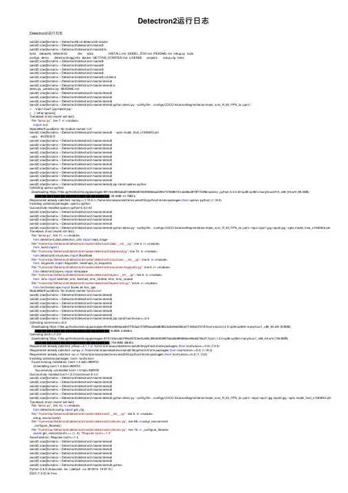
Detectron2运⾏⽇志Detectron2运⾏⽇志(wind2) star@xmatrix:~/Detectron2$ cd detectron2-master(wind2) star@xmatrix:~/Detectron2/detectron2-master$(wind2) star@xmatrix:~/Detectron2/detectron2-master$ lsbuild datasets detectron2 dev docs INSTALL.md MODEL_ZOO.md README.md setup.py toolsconfigs demo detectron2.egg-info docker GETTING_STARTED.md LICENSE projects setup.cfg tests(wind2) star@xmatrix:~/Detectron2/detectron2-master$(wind2) star@xmatrix:~/Detectron2/detectron2-master$(wind2) star@xmatrix:~/Detectron2/detectron2-master$(wind2) star@xmatrix:~/Detectron2/detectron2-master$(wind2) star@xmatrix:~/Detectron2/detectron2-master$ cd demo(wind2) star@xmatrix:~/Detectron2/detectron2-master/demo$(wind2) star@xmatrix:~/Detectron2/detectron2-master/demo$ lsdemo.py predictor.py README.md(wind2) star@xmatrix:~/Detectron2/detectron2-master/demo$(wind2) star@xmatrix:~/Detectron2/detectron2-master/demo$(wind2) star@xmatrix:~/Detectron2/detectron2-master/demo$(wind2) star@xmatrix:~/Detectron2/detectron2-master/demo$ python demo.py --config-file ../configs/COCO-InstanceSegmentation/mask_rcnn_R_50_FPN_3x.yaml \> --input input1.jpg input2.jpg \> [--other-options]Traceback (most recent call last):File "demo.py", line 7, in <module>import cv2ModuleNotFoundError: No module named 'cv2'(wind2) star@xmatrix:~/Detectron2/detectron2-master/demo$ --opts model_final_c10459X3.pkl--opts:未找到命令(wind2) star@xmatrix:~/Detectron2/detectron2-master/demo$(wind2) star@xmatrix:~/Detectron2/detectron2-master/demo$(wind2) star@xmatrix:~/Detectron2/detectron2-master/demo$(wind2) star@xmatrix:~/Detectron2/detectron2-master/demo$(wind2) star@xmatrix:~/Detectron2/detectron2-master/demo$(wind2) star@xmatrix:~/Detectron2/detectron2-master/demo$(wind2) star@xmatrix:~/Detectron2/detectron2-master/demo$(wind2) star@xmatrix:~/Detectron2/detectron2-master/demo$(wind2) star@xmatrix:~/Detectron2/detectron2-master/demo$(wind2) star@xmatrix:~/Detectron2/detectron2-master/demo$(wind2) star@xmatrix:~/Detectron2/detectron2-master/demo$(wind2) star@xmatrix:~/Detectron2/detectron2-master/demo$ pip install opencv-pythonCollecting opencv-pythonDownloading https:///packages/46/16/e49e5abd27d988e687634f58b0aa329fe737b686101cda48cd878f77429d/opencv_python-4.4.0.42-cp36-cp36m-manylinux2014_x86_64.whl (49.4MB)|████████████████████████████████| 49.4MB 10.7MB/sRequirement already satisfied: numpy>=1.13.3 in /home/star/anaconda3/envs/wind2/lib/python3.6/site-packages (from opencv-python) (1.18.0)Installing collected packages: opencv-pythonSuccessfully installed opencv-python-4.4.0.42(wind2) star@xmatrix:~/Detectron2/detectron2-master/demo$(wind2) star@xmatrix:~/Detectron2/detectron2-master/demo$(wind2) star@xmatrix:~/Detectron2/detectron2-master/demo$(wind2) star@xmatrix:~/Detectron2/detectron2-master/demo$(wind2) star@xmatrix:~/Detectron2/detectron2-master/demo$ python demo.py --config-file ../configs/COCO-InstanceSegmentation/mask_rcnn_R_50_FPN_3x.yaml -input input1.jpg input2.jpg --opts model_final_c10459X3.pkl Traceback (most recent call last):File "demo.py", line 11, in <module>from detectron2.data.detection_utils import read_imageFile "/home/star/Detectron2/detectron2-master/detectron2/data/__init__.py", line 4, in <module>from .build import (File "/home/star/Detectron2/detectron2-master/detectron2/data/build.py", line 12, in <module>from detectron2.structures import BoxModeFile "/home/star/Detectron2/detectron2-master/detectron2/structures/__init__.py", line 6, in <module>from .keypoints import Keypoints, heatmaps_to_keypointsFile "/home/star/Detectron2/detectron2-master/detectron2/structures/keypoints.py", line 6, in <module>from yers import interpolateFile "/home/star/Detectron2/detectron2-master/detectron2/layers/__init__.py", line 5, in <module>from .nms import batched_nms, batched_nms_rotated, nms, nms_rotatedFile "/home/star/Detectron2/detectron2-master/detectron2/layers/nms.py", line 6, in <module>from torchvision.ops import boxes as box_opsModuleNotFoundError: No module named 'torchvision'(wind2) star@xmatrix:~/Detectron2/detectron2-master/demo$(wind2) star@xmatrix:~/Detectron2/detectron2-master/demo$(wind2) star@xmatrix:~/Detectron2/detectron2-master/demo$(wind2) star@xmatrix:~/Detectron2/detectron2-master/demo$(wind2) star@xmatrix:~/Detectron2/detectron2-master/demo$(wind2) star@xmatrix:~/Detectron2/detectron2-master/demo$(wind2) star@xmatrix:~/Detectron2/detectron2-master/demo$ pip install torchvision==0.4Collecting torchvision==0.4Downloading https:///packages/06/e6/a564eba563f7ff53aa7318ff6aaa5bd8385cbda39ed55ba471e95af27d19/torchvision-0.4.0-cp36-cp36m-manylinux1_x86_64.whl (8.8MB)|████████████████████████████████| 8.8MB 3.6MB/sCollecting torch==1.2.0Downloading https:///packages/30/57/d5cceb0799c06733eefce80c395459f28970ebb9e896846ce96ab579a3f1/torch-1.2.0-cp36-cp36m-manylinux1_x86_64.whl (748.8MB)|████████████████████████████████| 748.9MB 38kB/sRequirement already satisfied: pillow>=4.1.1 in /home/star/anaconda3/envs/wind2/lib/python3.6/site-packages (from torchvision==0.4) (7.2.0)Requirement already satisfied: numpy in /home/star/anaconda3/envs/wind2/lib/python3.6/site-packages (from torchvision==0.4) (1.18.0)Requirement already satisfied: six in /home/star/anaconda3/envs/wind2/lib/python3.6/site-packages (from torchvision==0.4) (1.13.0)Installing collected packages: torch, torchvisionFound existing installation: torch 1.4.0a0+39297bfUninstalling torch-1.4.0a0+39297bf:Successfully uninstalled torch-1.4.0a0+39297bfSuccessfully installed torch-1.2.0 torchvision-0.4.0(wind2) star@xmatrix:~/Detectron2/detectron2-master/demo$(wind2) star@xmatrix:~/Detectron2/detectron2-master/demo$(wind2) star@xmatrix:~/Detectron2/detectron2-master/demo$(wind2) star@xmatrix:~/Detectron2/detectron2-master/demo$(wind2) star@xmatrix:~/Detectron2/detectron2-master/demo$(wind2) star@xmatrix:~/Detectron2/detectron2-master/demo$ python demo.py --config-file ../configs/COCO-InstanceSegmentation/mask_rcnn_R_50_FPN_3x.yaml --input input1.jpg input2.jpg --opts model_final_c10459X3.pkl Traceback (most recent call last):File "demo.py", line 10, in <module>from detectron2.config import get_cfgFile "/home/star/Detectron2/detectron2-master/detectron2/__init__.py", line 5, in <module>setup_environment()File "/home/star/Detectron2/detectron2-master/detectron2/utils/env.py", line 98, in setup_environment_configure_libraries()File "/home/star/Detectron2/detectron2-master/detectron2/utils/env.py", line 76, in _configure_librariesassert get_version(torch) >= (1, 4), "Requires torch>=1.4"AssertionError: Requires torch>=1.4(wind2) star@xmatrix:~/Detectron2/detectron2-master/demo$(wind2) star@xmatrix:~/Detectron2/detectron2-master/demo$(wind2) star@xmatrix:~/Detectron2/detectron2-master/demo$(wind2) star@xmatrix:~/Detectron2/detectron2-master/demo$(wind2) star@xmatrix:~/Detectron2/detectron2-master/demo$(wind2) star@xmatrix:~/Detectron2/detectron2-master/demo$(wind2) star@xmatrix:~/Detectron2/detectron2-master/demo$ pythonPython 3.6.9 |Anaconda, Inc.| (default, Jul 30 2019, 19:07:31)[GCC 7.3.0] on linuxType "help", "copyright", "credits"or"license"for more information.>>>>>>>>> import torch>>>>>> print(torch.__version__)1.2.0>>>>>>>>>>>>>>> print(torch.__version__)1.2.0>>>>>>>>>>>> exit();(wind2) star@xmatrix:~/Detectron2/detectron2-master/demo$(wind2) star@xmatrix:~/Detectron2/detectron2-master/demo$(wind2) star@xmatrix:~/Detectron2/detectron2-master/demo$(wind2) star@xmatrix:~/Detectron2/detectron2-master/demo$(wind2) star@xmatrix:~/Detectron2/detectron2-master/demo$ pip uninstall torchvisionUninstalling torchvision-0.4.0:Would remove:/home/star/anaconda3/envs/wind2/lib/python3.6/site-packages/torchvision-0.4.0.dist-info/*/home/star/anaconda3/envs/wind2/lib/python3.6/site-packages/torchvision/*Proceed (y/n)? ySuccessfully uninstalled torchvision-0.4.0(wind2) star@xmatrix:~/Detectron2/detectron2-master/demo$(wind2) star@xmatrix:~/Detectron2/detectron2-master/demo$(wind2) star@xmatrix:~/Detectron2/detectron2-master/demo$(wind2) star@xmatrix:~/Detectron2/detectron2-master/demo$(wind2) star@xmatrix:~/Detectron2/detectron2-master/demo$(wind2) star@xmatrix:~/Detectron2/detectron2-master/demo$ pip install torchvision==0.5Collecting torchvision==0.5Downloading https:///packages/7e/90/6141bf41f5655c78e24f40f710fdd4f8a8aff6c8b7c6f0328240f649bdbe/torchvision-0.5.0-cp36-cp36m-manylinux1_x86_64.whl (4.0MB)|████████████████████████████████| 4.0MB 3.2MB/sRequirement already satisfied: pillow>=4.1.1 in /home/star/anaconda3/envs/wind2/lib/python3.6/site-packages (from torchvision==0.5) (7.2.0)Collecting torch==1.4.0Downloading https:///packages/24/19/4804aea17cd136f1705a5e98a00618cb8f6ccc375ad8bfa437408e09d058/torch-1.4.0-cp36-cp36m-manylinux1_x86_64.whl (753.4MB)|████████████████████████████████| 753.4MB 32kB/sRequirement already satisfied: numpy in /home/star/anaconda3/envs/wind2/lib/python3.6/site-packages (from torchvision==0.5) (1.18.0)Requirement already satisfied: six in /home/star/anaconda3/envs/wind2/lib/python3.6/site-packages (from torchvision==0.5) (1.13.0)Installing collected packages: torch, torchvisionFound existing installation: torch 1.2.0Uninstalling torch-1.2.0:Successfully uninstalled torch-1.2.0Successfully installed torch-1.4.0 torchvision-0.5.0(wind2) star@xmatrix:~/Detectron2/detectron2-master/demo$(wind2) star@xmatrix:~/Detectron2/detectron2-master/demo$(wind2) star@xmatrix:~/Detectron2/detectron2-master/demo$(wind2) star@xmatrix:~/Detectron2/detectron2-master/demo$(wind2) star@xmatrix:~/Detectron2/detectron2-master/demo$(wind2) star@xmatrix:~/Detectron2/detectron2-master/demo$(wind2) star@xmatrix:~/Detectron2/detectron2-master/demo$(wind2) star@xmatrix:~/Detectron2/detectron2-master/demo$ python demo.py --config-file ../configs/COCO-InstanceSegmentation/mask_rcnn_R_50_FPN_3x.yaml --input input1.jpg input2.jpg --opts model_final_c10459X3.pkl Traceback (most recent call last):File "demo.py", line 11, in <module>from detectron2.data.detection_utils import read_imageFile "/home/star/Detectron2/detectron2-master/detectron2/data/__init__.py", line 4, in <module>from .build import (File "/home/star/Detectron2/detectron2-master/detectron2/data/build.py", line 12, in <module>from detectron2.structures import BoxModeFile "/home/star/Detectron2/detectron2-master/detectron2/structures/__init__.py", line 6, in <module>from .keypoints import Keypoints, heatmaps_to_keypointsFile "/home/star/Detectron2/detectron2-master/detectron2/structures/keypoints.py", line 6, in <module>from yers import interpolateFile "/home/star/Detectron2/detectron2-master/detectron2/layers/__init__.py", line 3, in <module>from .deform_conv import DeformConv, ModulatedDeformConvFile "/home/star/Detectron2/detectron2-master/detectron2/layers/deform_conv.py", line 10, in <module>from detectron2 import _CImportError: /home/star/Detectron2/detectron2-master/detectron2/_C.cpython-36m-x86_64-linux-gnu.so: undefined symbol: _ZN3c107Warning4warnENS_14SourceLocationERKNSt7__cxx1112basic_stringIcSt11char_traitsIcESaIcEEE (wind2) star@xmatrix:~/Detectron2/detectron2-master/demo$(wind2) star@xmatrix:~/Detectron2/detectron2-master/demo$(wind2) star@xmatrix:~/Detectron2/detectron2-master/demo$(wind2) star@xmatrix:~/Detectron2/detectron2-master/demo$。
927fatal memory error摘要:1.介绍“927fatal memory error”的含义2.分析“927fatal memory error”的原因3.探讨解决“927fatal memory error”的方法4.总结“927fatal memory error”的影响和处理方式正文:一、“927fatal memory error”的含义“927fatal memory error”是一个常见的计算机错误,通常表示程序因为内存问题而崩溃。
具体来说,这个错误意味着程序试图访问未分配给它的内存地址,从而导致程序异常终止。
二、“927fatal memory error”的原因“927fatal memory error”的出现通常有以下几个原因:1.空指针引用:程序试图访问内存地址,但是该地址为空,没有分配给任何变量。
2.内存泄漏:程序在运行过程中,分配的内存没有被及时释放,导致内存占用过多,最终引发内存错误。
3.缓冲区溢出:程序向缓冲区写入数据时,超过了缓冲区的容量,导致数据覆盖到相邻的内存区域。
4.使用未初始化的变量:程序在访问某个变量时,该变量尚未被初始化,其值可能是未定义的,从而导致内存错误。
三、解决“927fatal memory error”的方法为了避免或解决“927fatal memory error”,可以采取以下措施:1.检查代码中的内存分配和释放,确保所有的内存使用都是正确的。
2.使用调试工具,如GDB,查找程序崩溃的具体位置,分析错误原因。
3.对于空指针引用,可以采用空值检查的方法,确保在访问指针前,指针不为空。
4.对于内存泄漏,可以使用内存检测工具,如Valgrind,查找泄漏的内存并及时释放。
5.对于缓冲区溢出,可以通过限制写入数据的长度,或者使用动态缓冲区来避免溢出。
6.对于使用未初始化的变量,需要确保在访问变量前对其进行初始化。
四、总结“927fatal memory error”是程序开发过程中常见的内存错误,对程序的稳定性和可靠性产生严重影响。
dbmind慢sql发现原理
DBMind慢SQL发现原理是什么?在数据库运行中,由于各种原因,可能会出现一些查询语句的执行速度较慢的情况,这些SQL被称为慢SQL。
慢SQL的存在会影响数据库的性能和稳定性,需要尽快发现和解决。
DBMind慢SQL发现原理就是通过分析数据库运行日志和
查询计划,找出执行速度较慢的SQL语句,并进行分析和优化。
具体来说,它会采集数据库的运行日志,并记录下每个查询语句的执行时间、执行次数、执行计划等信息,然后根据这些信息进行分析和排查。
通过对慢SQL的分析,可以发现存在的性能瓶颈和潜在的问题,并提供相应的优化建议。
这样可以帮助数据库管理员快速解决慢SQL问题,提高数据库性能和稳定性。
- 1 -。
3GPP TS 36.521-1 V14.4.0 (2017-09)Technical Specification3rd Generation Partnership Project; Technical Specification Group Radio Access Network; Evolved Universal Terrestrial Radio Access (E-UTRA);User Equipment (UE) conformance specification;Radio transmission and reception;Part 1: Conformance Testing(Release 14)The present document has been developed within the 3rd Generation Partnership Project (3GPP TM) and may be further elaborated for the purposes of 3GPP.KeywordsUMTS LTE3GPPPostal address3GPP support office address650 Route des Lucioles - Sophia AntipolisValbonne - FRANCETel.: +33 4 92 94 42 00 Fax: +33 4 93 65 47 16InternetCopyright NotificationNo part may be reproduced except as authorized by written permission.The copyright and the foregoing restriction extend to reproduction in all media.© 2017, 3GPP Organizational Partners (ARIB, ATIS, CCSA, ETSI, TSDSI, TTA, TTC).All rights reserved.UMTS™ is a Trade Mark of ETSI registered for the benefit of its members3GPP™ is a Trade Mark of ETSI registered for the benefit of its Members and of the 3GPP Organizational Partners LTE™ is a Trade Mark of ETSI registered for the benefit of its Members a nd of the 3GPP Organizational Partners GSM® and the GSM logo are registered and owned by the GSM AssociationContentsForeword (92)Introduction (92)1Scope (93)2References (94)3Definitions, symbols and abbreviations (96)3.1Definitions (96)3.2Symbols (98)3.3Abbreviations (100)4General (103)4.1Categorization of test requirements in CA, UL-MIMO, ProSe, Dual Connectivity, UE category 0, UEcategory M1, UE category 1bis, UE category NB1 and V2X Communication (104)4.2RF requirements in later releases (105)5Frequency bands and channel arrangement (106)5.1General (106)5.2Operating bands (106)5.2A Operating bands for CA (108)5.2B Operating bands for UL-MIMO (116)5.2C Operating bands for Dual Connectivity (116)5.2D Operating bands for ProSe (117)5.2E Operating bands for UE category 0 and UE category M1 (118)5.2F Operating bands for UE category NB1 (118)5.2G Operating bands for V2X Communication (118)5.3TX–RX frequency separation (119)5.3A TX–RX frequency separation for CA (120)5.4Channel arrangement (120)5.4.1Channel spacing (120)5.4.1A Channel spacing for CA (121)5.4.1F Channel spacing for UE category NB1 (121)5.4.2Channel bandwidth (121)5.4.2.1Channel bandwidths per operating band (122)5.4.2A Channel bandwidth for CA (124)5.4.2A.1Channel bandwidths per operating band for CA (126)5.4.2B Channel bandwidth for UL-MIMO (171)5.4.2B.1Channel bandwidths per operating band for UL- MIMO (171)5.4.2C Channel bandwidth for Dual Connectivity (171)5.4.2D Channel bandwidth for ProSe (171)5.4.2D.1Channel bandwidths per operating band for ProSe (171)5.4.2F Channel bandwidth for category NB1 (172)5.4.2G Channel bandwidth for V2X Communication (173)5.4.2G.1Channel bandwidths per operating band for V2X Communication (173)5.4.3Channel raster (174)5.4.3A Channel raster for CA (175)5.4.3F Channel raster for UE category NB1 (175)5.4.4Carrier frequency and EARFCN (175)5.4.4F Carrier frequency and EARFCN for category NB1 (177)6Transmitter Characteristics (179)6.1General (179)6.2Transmit power (180)6.2.1Void (180)6.2.2UE Maximum Output Power (180)6.2.2.1Test purpose (180)6.2.2.4Test description (182)6.2.2.4.1Initial condition (182)6.2.2.4.2Test procedure (183)6.2.2.4.3Message contents (183)6.2.2.5Test requirements (183)6.2.2_1Maximum Output Power for HPUE (185)6.2.2_1.1Test purpose (185)6.2.2_1.2Test applicability (185)6.2.2_1.3Minimum conformance requirements (185)6.2.2_1.4Test description (185)6.2.2_1.5Test requirements (186)6.2.2A UE Maximum Output Power for CA (187)6.2.2A.0Minimum conformance requirements (187)6.2.2A.1UE Maximum Output Power for CA (intra-band contiguous DL CA and UL CA) (189)6.2.2A.1.1Test purpose (189)6.2.2A.1.2Test applicability (189)6.2.2A.1.3Minimum conformance requirements (189)6.2.2A.1.4Test description (189)6.2.2A.1.5Test Requirements (191)6.2.2A.2UE Maximum Output Power for CA (inter-band DL CA and UL CA) (192)6.2.2A.2.1Test purpose (192)6.2.2A.2.2Test applicability (192)6.2.2A.2.3Minimum conformance requirements (192)6.2.2A.2.4Test description (192)6.2.2A.2.5Test Requirements (194)6.2.2A.3UE Maximum Output Power for CA (intra-band non-contiguous DL CA and UL CA) (196)6.2.2A.4.1UE Maximum Output Power for CA (intra-band contiguous 3DL CA and 3UL CA) (196)6.2.2A.4.1.1Test purpose (196)6.2.2A.4.1.2Test applicability (196)6.2.2A.4.1.3Minimum conformance requirements (196)6.2.2A.4.1.4Test description (196)6.2.2A.4.1.5Test Requirements (198)6.2.2A.4.2UE Maximum Output Power for CA (inter-band 3DL CA and 3UL CA) (198)6.2.2A.4.2.1Test purpose (199)6.2.2A.4.2.2Test applicability (199)6.2.2A.4.2.3Minimum conformance requirements (199)6.2.2A.4.2.4Test description (199)6.2.2A.4.2.5Test Requirements (201)6.2.2B UE Maximum Output Power for UL-MIMO (201)6.2.2B.1Test purpose (201)6.2.2B.2Test applicability (202)6.2.2B.3Minimum conformance requirements (202)6.2.2B.4Test description (204)6.2.2B.4.1Initial condition (204)6.2.2B.4.2Test procedure (205)6.2.2B.4.3Message contents (205)6.2.2B.5Test requirements (205)6.2.2B_1HPUE Maximum Output Power for UL-MIMO (207)6.2.2B_1.1Test purpose (207)6.2.2B_1.2Test applicability (207)6.2.2B_1.3Minimum conformance requirements (207)6.2.2B_1.4Test description (207)6.2.2B_1.5Test requirements (208)6.2.2C 2096.2.2D UE Maximum Output Power for ProSe (209)6.2.2D.0Minimum conformance requirements (209)6.2.2D.1UE Maximum Output Power for ProSe Discovery (209)6.2.2D.1.1Test purpose (209)6.2.2D.1.2Test applicability (209)6.2.2D.1.3Minimum Conformance requirements (209)6.2.2D.2UE Maximum Output Power for ProSe Direct Communication (211)6.2.2D.2.1Test purpose (211)6.2.2D.2.2Test applicability (211)6.2.2D.2.3Minimum conformance requirements (211)6.2.2D.2.4Test description (211)6.2.2E UE Maximum Output Power for UE category 0 (212)6.2.2E.1Test purpose (212)6.2.2E.2Test applicability (212)6.2.2E.3Minimum conformance requirements (212)6.2.2E.4Test description (212)6.2.2E.4.3Message contents (213)6.2.2E.5Test requirements (213)6.2.2EA UE Maximum Output Power for UE category M1 (215)6.2.2EA.1Test purpose (215)6.2.2EA.2Test applicability (215)6.2.2EA.3Minimum conformance requirements (215)6.2.2EA.4Test description (216)6.2.2EA.4.3Message contents (217)6.2.2EA.5Test requirements (217)6.2.2F UE Maximum Output Power for category NB1 (218)6.2.2F.1Test purpose (218)6.2.2F.2Test applicability (218)6.2.2F.3Minimum conformance requirements (218)6.2.2F.4Test description (219)6.2.2F.4.1Initial condition (219)6.2.2F.4.2Test procedure (220)6.2.2F.4.3Message contents (220)6.2.2F.5Test requirements (220)6.2.2G UE Maximum Output Power for V2X Communication (221)6.2.2G.1UE Maximum Output Power for V2X Communication / Non-concurrent with E-UTRA uplinktransmission (221)6.2.2G.1.1Test purpose (221)6.2.2G.1.2Test applicability (221)6.2.2G.1.3Minimum conformance requirements (221)6.2.2G.1.4Test description (222)6.2.2G.1.4.1Initial conditions (222)6.2.2G.1.4.2Test procedure (222)6.2.2G.1.4.3Message contents (222)6.2.2G.1.5Test requirements (223)6.2.2G.2UE Maximum Output Power for V2X Communication / Simultaneous E-UTRA V2X sidelinkand E-UTRA uplink transmission (223)6.2.2G.2.1Test purpose (223)6.2.2G.2.2Test applicability (223)6.2.2G.2.3Minimum conformance requirements (223)6.2.2G.2.4Test description (224)6.2.2G.2.4.1Initial conditions (224)6.2.2G.2.4.2Test procedure (225)6.2.2G.2.4.3Message contents (226)6.2.2G.2.5Test requirements (226)6.2.3Maximum Power Reduction (MPR) (226)6.2.3.1Test purpose (226)6.2.3.2Test applicability (226)6.2.3.3Minimum conformance requirements (227)6.2.3.4Test description (227)6.2.3.4.1Initial condition (227)6.2.3.4.2Test procedure (228)6.2.3.4.3Message contents (228)6.2.3.5Test requirements (229)6.2.3_1Maximum Power Reduction (MPR) for HPUE (231)6.2.3_1.1Test purpose (231)6.2.3_1.4Test description (232)6.2.3_1.5Test requirements (232)6.2.3_2Maximum Power Reduction (MPR) for Multi-Cluster PUSCH (232)6.2.3_2.1Test purpose (232)6.2.3_2.2Test applicability (232)6.2.3_2.3Minimum conformance requirements (233)6.2.3_2.4Test description (233)6.2.3_2.4.1Initial condition (233)6.2.3_2.4.2Test procedure (234)6.2.3_2.4.3Message contents (234)6.2.3_2.5Test requirements (234)6.2.3_3Maximum Power Reduction (MPR) for UL 64QAM (235)6.2.3_3.1Test purpose (236)6.2.3_3.2Test applicability (236)6.2.3_3.3Minimum conformance requirements (236)6.2.3_3.4Test description (236)6.2.3_3.4.1Initial condition (236)6.2.3_3.4.2Test procedure (237)6.2.3_3.4.3Message contents (237)6.2.3_3.5Test requirements (238)6.2.3_4Maximum Power Reduction (MPR) for Multi-Cluster PUSCH with UL 64QAM (240)6.2.3_4.1Test purpose (240)6.2.3_4.2Test applicability (240)6.2.3_4.3Minimum conformance requirements (240)6.2.3_4.4Test description (241)6.2.3_4.4.1Initial condition (241)6.2.3_4.4.2Test procedure (242)6.2.3_4.4.3Message contents (242)6.2.3_4.5Test requirements (242)6.2.3A Maximum Power Reduction (MPR) for CA (243)6.2.3A.1Maximum Power Reduction (MPR) for CA (intra-band contiguous DL CA and UL CA) (243)6.2.3A.1.1Test purpose (243)6.2.3A.1.2Test applicability (243)6.2.3A.1.3Minimum conformance requirements (244)6.2.3A.1.4Test description (245)6.2.3A.1.5Test Requirements (248)6.2.3A.1_1Maximum Power Reduction (MPR) for CA (intra-band contiguous DL CA and UL CA) for UL64QAM (250)6.2.3A.1_1.1Test purpose (251)6.2.3A.1_1.2Test applicability (251)6.2.3A.1_1.3Minimum conformance requirements (251)6.2.3A.1_1.4Test description (252)6.2.3A.1_1.5Test requirement (254)6.2.3A.2Maximum Power Reduction (MPR) for CA (inter-band DL CA and UL CA) (255)6.2.3A.2.1Test purpose (255)6.2.3A.2.2Test applicability (255)6.2.3A.2.3Minimum conformance requirements (255)6.2.3A.2.4Test description (256)6.2.3A.2.5Test Requirements (260)6.2.3A.2_1Maximum Power Reduction (MPR) for CA (inter-band DL CA and UL CA) for UL 64QAM (263)6.2.3A.2_1.1Test purpose (263)6.2.3A.2_1.2Test applicability (263)6.2.3A.2_1.3Minimum conformance requirements (263)6.2.3A.2_1.4Test description (264)6.2.3A.2_1.5Test Requirements (266)6.2.3A.3Maximum Power Reduction (MPR) for CA (intra-band non-contiguous DL CA and UL CA) (267)6.2.3A.3.1Test purpose (267)6.2.3A.3.2Test applicability (267)6.2.3A.3.3Minimum conformance requirements (268)6.2.3A.3.4Test description (268)6.2.3A.3_1Maximum Power Reduction (MPR) for CA (intra-band non-contiguous DL CA and UL CA) forUL 64QAM (270)6.2.3A.3_1.1Test purpose (270)6.2.3A.3_1.2Test applicability (270)6.2.3A.3_1.3Minimum conformance requirements (270)6.2.3A.3_1.4Test description (271)6.2.3A.3_1.5Test Requirements (272)6.2.3B Maximum Power Reduction (MPR) for UL-MIMO (272)6.2.3B.1Test purpose (272)6.2.3B.2Test applicability (272)6.2.3B.3Minimum conformance requirements (273)6.2.3B.4Test description (273)6.2.3B.4.1Initial condition (273)6.2.3B.4.2Test procedure (274)6.2.3B.4.3Message contents (275)6.2.3B.5Test requirements (275)6.2.3D UE Maximum Output Power for ProSe (277)6.2.3D.0Minimum conformance requirements (277)6.2.3D.1Maximum Power Reduction (MPR) for ProSe Discovery (278)6.2.3D.1.1Test purpose (278)6.2.3D.1.2Test applicability (278)6.2.3D.1.3Minimum conformance requirements (278)6.2.3D.1.4Test description (278)6.2.3D.1.4.1Initial condition (278)6.2.3D.1.4.2Test procedure (279)6.2.3D.1.4.3Message contents (279)6.2.3D.1.5Test requirements (280)6.2.3D.2Maximum Power Reduction (MPR) ProSe Direct Communication (281)6.2.3D.2.1Test purpose (282)6.2.3D.2.2Test applicability (282)6.2.3D.2.3Minimum conformance requirements (282)6.2.3D.2.4Test description (282)6.2.3D.2.4.1Initial conditions (282)6.2.3D.2.4.2Test procedure (282)6.2.3D.2.4.3Message contents (282)6.2.3D.2.5Test requirements (282)6.2.3E Maximum Power Reduction (MPR) for UE category 0 (282)6.2.3E.1Test purpose (282)6.2.3E.2Test applicability (282)6.2.3E.3Minimum conformance requirements (282)6.2.3E.4Test description (282)6.2.3E.4.1Initial condition (282)6.2.3E.4.2Test procedure (283)6.2.3E.4.3Message contents (283)6.2.3E.5Test requirements (283)6.2.3EA Maximum Power Reduction (MPR) for UE category M1 (284)6.2.3EA.1Test purpose (284)6.2.3EA.2Test applicability (284)6.2.3EA.3Minimum conformance requirements (284)6.2.3EA.4Test description (285)6.2.3EA.4.1Initial condition (285)6.2.3EA.4.2Test procedure (287)6.2.3EA.4.3Message contents (287)6.2.3EA.5Test requirements (287)6.2.3F Maximum Power Reduction (MPR) for category NB1 (290)6.2.3F.1Test purpose (290)6.2.3F.2Test applicability (290)6.2.3F.3Minimum conformance requirements (290)6.2.3F.4Test description (291)6.2.3F.4.1Initial condition (291)6.2.3F.5Test requirements (292)6.2.3G Maximum Power Reduction (MPR) for V2X communication (292)6.2.3G.1Maximum Power Reduction (MPR) for V2X Communication / Power class 3 (293)6.2.3G.1.1Maximum Power Reduction (MPR) for V2X Communication / Power class 3 / Contiguousallocation of PSCCH and PSSCH (293)6.2.3G.1.1.1Test purpose (293)6.2.3G.1.1.2Test applicability (293)6.2.3G.1.1.3Minimum conformance requirements (293)6.2.3G.1.1.4Test description (293)6.2.3G.1.1.4.1Initial condition (293)6.2.3G.1.1.4.2Test procedure (294)6.2.3G.1.1.4.3Message contents (294)6.2.3G.1.1.5Test Requirements (294)6.2.3G.1.2 2956.2.3G.1.3Maximum Power Reduction (MPR) for V2X Communication / Power class 3 / SimultaneousE-UTRA V2X sidelink and E-UTRA uplink transmission (295)6.2.3G.1.3.1Test purpose (295)6.2.3G.1.3.2Test applicability (295)6.2.3G.1.3.3Minimum conformance requirements (295)6.2.3G.1.3.4Test description (295)6.2.3G.1.3.4.1Initial conditions (295)6.2.3G.1.3.4.2Test procedure (296)6.2.3G.1.3.4.3Message contents (297)6.2.3G.1.3.5Test requirements (297)6.2.4Additional Maximum Power Reduction (A-MPR) (297)6.2.4.1Test purpose (297)6.2.4.2Test applicability (297)6.2.4.3Minimum conformance requirements (298)6.2.4.4Test description (310)6.2.4.4.1Initial condition (310)6.2.4.4.2Test procedure (339)6.2.4.4.3Message contents (339)6.2.4.5Test requirements (344)6.2.4_1Additional Maximum Power Reduction (A-MPR) for HPUE (373)6.2.4_1.2Test applicability (374)6.2.4_1.3Minimum conformance requirements (374)6.2.4_1.4Test description (375)6.2.4_1.5Test requirements (376)6.2.4_2Additional Maximum Power Reduction (A-MPR) for UL 64QAM (378)6.2.4_2.1Test purpose (378)6.2.4_2.2Test applicability (378)6.2.4_2.3Minimum conformance requirements (378)6.2.4_2.4Test description (378)6.2.4_2.4.1Initial condition (378)6.2.4_2.4.2Test procedure (392)6.2.4_2.4.3Message contents (392)6.2.4_2.5Test requirements (392)6.2.4_3Additional Maximum Power Reduction (A-MPR) with PUSCH frequency hopping (404)6.2.4_3.1Test purpose (404)6.2.4_3.2Test applicability (404)6.2.4_3.3Minimum conformance requirements (405)6.2.4_3.4Test description (405)6.2.4_3.5Test requirements (406)6.2.4A Additional Maximum Power Reduction (A-MPR) for CA (407)6.2.4A.1Additional Maximum Power Reduction (A-MPR) for CA (intra-band contiguous DL CA and ULCA) (407)6.2.4A.1.1Test purpose (407)6.2.4A.1.2Test applicability (407)6.2.4A.1.3Minimum conformance requirements (407)6.2.4A.1.3.5A-MPR for CA_NS_05 for CA_38C (411)6.2.4A.1.4Test description (413)6.2.4A.1.5Test requirements (419)6.2.4A.1_1Additional Maximum Power Reduction (A-MPR) for CA (intra-band contiguous DL CA and ULCA) for UL 64QAM (425)6.2.4A.1_1.1Test purpose (425)6.2.4A.1_1.2Test applicability (425)6.2.4A.1_1.3Minimum conformance requirements (426)6.2.4A.1_1.3.5A-MPR for CA_NS_05 for CA_38C (429)6.2.4A.1_1.3.6A-MPR for CA_NS_06 for CA_7C (430)6.2.4A.1_1.3.7A-MPR for CA_NS_07 for CA_39C (431)6.2.4A.1_1.3.8A-MPR for CA_NS_08 for CA_42C (432)6.2.4A.1_1.4Test description (432)6.2.4A.1_1.5Test requirements (437)6.2.4A.2Additional Maximum Power Reduction (A-MPR) for CA (inter-band DL CA and UL CA) (443)6.2.4A.2.1Test purpose (443)6.2.4A.2.2Test applicability (444)6.2.4A.2.3Minimum conformance requirements (444)6.2.4A.2.4Test description (444)6.2.4A.2.4.1Initial conditions (444)6.2.4A.2.4.2Test procedure (457)6.2.4A.2.4.3Message contents (458)6.2.4A.2.5Test requirements (461)6.2.4A.3Additional Maximum Power Reduction (A-MPR) for CA (intra-band non-contiguous DL CAand UL CA) (466)6.2.4A.3.1Minimum conformance requirements (466)6.2.4A.2_1Additional Maximum Power Reduction (A-MPR) for CA (inter-band DL CA and UL CA) forUL 64QAM (466)6.2.4A.2_1.1Test purpose (466)6.2.4A.2_1.2Test applicability (466)6.2.4A.2_1.3Minimum conformance requirements (467)6.2.4A.2_1.4Test description (467)6.2.4A.2_1.4.1Initial conditions (467)6.2.4A.2_1.4.2Test procedure (479)6.2.4A.2_1.4.3Message contents (480)6.2.4A.2_1.5Test requirements (480)6.2.4B Additional Maximum Power Reduction (A-MPR) for UL-MIMO (484)6.2.4B.1Test purpose (484)6.2.4B.2Test applicability (485)6.2.4B.3Minimum conformance requirements (485)6.2.4B.4Test description (485)6.2.4B.4.1Initial condition (485)6.2.4B.4.2Test procedure (508)6.2.4B.4.3Message contents (508)6.2.4B.5Test requirements (508)6.2.4E Additional Maximum Power Reduction (A-MPR) for UE category 0 (530)6.2.4E.1Test purpose (530)6.2.4E.2Test applicability (531)6.2.4E.3Minimum conformance requirements (531)6.2.4E.4Test description (531)6.2.4E.4.1Initial condition (531)6.2.4E.4.2Test procedure (535)6.2.4E.4.3Message contents (535)6.2.4E.5Test requirements (536)6.2.4EA Additional Maximum Power Reduction (A-MPR) for UE category M1 (542)6.2.4EA.1Test purpose (542)6.2.4EA.2Test applicability (542)6.2.4EA.3Minimum conformance requirements (543)6.2.4EA.4Test description (544)6.2.4EA.4.1Initial condition (544)6.2.4EA.4.2Test procedure (552)6.2.4G Additional Maximum Power Reduction (A-MPR) for V2X Communication (562)6.2.4G.1Additional Maximum Power Reduction (A-MPR) for V2X Communication / Non-concurrentwith E-UTRA uplink transmissions (562)6.2.4G.1.1Test purpose (562)6.2.4G.1.2Test applicability (562)6.2.4G.1.3Minimum conformance requirements (563)6.2.4G.1.4Test description (563)6.2.4G.1.4.1Initial condition (563)6.2.4G.1.4.2Test procedure (564)6.2.4G.1.4.3Message contents (564)6.2.4G.1.5Test Requirements (564)6.2.5Configured UE transmitted Output Power (564)6.2.5.1Test purpose (564)6.2.5.2Test applicability (564)6.2.5.3Minimum conformance requirements (564)6.2.5.4Test description (594)6.2.5.4.1Initial conditions (594)6.2.5.4.2Test procedure (595)6.2.5.4.3Message contents (595)6.2.5.5Test requirement (596)6.2.5_1Configured UE transmitted Output Power for HPUE (596)6.2.5_1.1Test purpose (596)6.2.5_1.2Test applicability (597)6.2.5_1.3Minimum conformance requirements (597)6.2.5_1.4Test description (597)6.2.5_1.4.1Initial conditions (597)6.2.5_1.4.2Test procedure (597)6.2.5_1.4.3Message contents (597)6.2.5_1.5Test requirement (598)6.2.5A Configured transmitted power for CA (599)6.2.5A.1Configured UE transmitted Output Power for CA (intra-band contiguous DL CA and UL CA) (599)6.2.5A.1.1Test purpose (599)6.2.5A.1.2Test applicability (599)6.2.5A.1.3Minimum conformance requirements (599)6.2.5A.1.4Test description (601)6.2.5A.1.5Test requirement (602)6.2.5A.2Void (603)6.2.5A.3Configured UE transmitted Output Power for CA (inter-band DL CA and UL CA) (603)6.2.5A.3.1Test purpose (603)6.2.5A.3.2Test applicability (603)6.2.5A.3.3Minimum conformance requirements (603)6.2.5A.3.4Test description (605)6.2.5A.3.5Test requirement (606)6.2.5A.4Configured UE transmitted Output Power for CA (intra-band non-contiguous DL CA and ULCA) (607)6.2.5A.4.1Test purpose (607)6.2.5A.4.2Test applicability (607)6.2.5A.4.3Minimum conformance requirements (607)6.2.5A.4.4Test description (608)6.2.5A.4.5Test requirement (610)6.2.5B Configured UE transmitted Output Power for UL-MIMO (611)6.2.5B.1Test purpose (611)6.2.5B.2Test applicability (611)6.2.5B.3Minimum conformance requirements (611)6.2.5B.4Test description (612)6.2.5B.4.1Initial conditions (612)6.2.5B.4.2Test procedure (612)6.2.5B.4.3Message contents (613)6.2.5B.5Test requirement (613)6.2.5E Configured UE transmitted Output Power for UE category 0 (614)6.2.5E.4.1Initial conditions (614)6.2.5E.4.2Test procedure (614)6.2.5E.4.3Message contents (614)6.2.5E.5Test requirement (615)6.2.5EA Configured UE transmitted Power for UE category M1 (615)6.2.5EA.1Test purpose (615)6.2.5EA.2Test applicability (615)6.2.5EA.3Minimum conformance requirements (615)6.2.5EA.4Test description (616)6.2.5EA.4.1Initial condition (616)6.2.5EA.4.2Test procedure (617)6.2.5EA.4.3Message contents (617)6.2.5EA.5Test requirements (617)6.2.5F Configured UE transmitted Output Power for UE category NB1 (618)6.2.5F.1Test purpose (618)6.2.5F.2Test applicability (618)6.2.5F.3Minimum conformance requirements (618)6.2.5F.4Test description (619)6.2.5F.4.1Initial conditions (619)6.2.5F.4.2Test procedure (620)6.2.5F.4.3Message contents (620)6.2.5F.5Test requirement (620)6.2.5G Configured UE transmitted Output Power for V2X Communication (620)6.2.5G.1Configured UE transmitted Output Power for V2X Communication / Non-concurrent with E-UTRA uplink transmission (621)6.2.5G.1.1Test purpose (621)6.2.5G.1.2Test applicability (621)6.2.5G.1.3Minimum conformance requirements (621)6.2.5G.1.4Test description (622)6.2.5G.1.4.1Initial conditions (622)6.2.5G.1.4.2Test procedure (622)6.2.5G.1.4.3Message contents (622)6.2.5G.1.5Test requirements (622)6.2.5G.2Configured UE transmitted Output Power for V2X Communication / Simultaneous E-UTRAV2X sidelink and E-UTRA uplink transmission (622)6.2.5G.2.1Test purpose (623)6.2.5G.2.2Test applicability (623)6.2.5G.2.3Minimum conformance requirements (623)6.2.5G.2.4Test description (625)6.2.5G.2.4.1Initial conditions (625)6.2.5G.2.4.2Test procedure (626)6.2.5G.2.4.3Message contents (626)6.2.5G.2.5Test requirements (626)6.3Output Power Dynamics (627)6.3.1Void (627)6.3.2Minimum Output Power (627)6.3.2.1Test purpose (627)6.3.2.2Test applicability (627)6.3.2.3Minimum conformance requirements (627)6.3.2.4Test description (627)6.3.2.4.1Initial conditions (627)6.3.2.4.2Test procedure (628)6.3.2.4.3Message contents (628)6.3.2.5Test requirement (628)6.3.2A Minimum Output Power for CA (629)6.3.2A.0Minimum conformance requirements (629)6.3.2A.1Minimum Output Power for CA (intra-band contiguous DL CA and UL CA) (629)6.3.2A.1.1Test purpose (629)6.3.2A.1.4.2Test procedure (631)6.3.2A.1.4.3Message contents (631)6.3.2A.1.5Test requirements (631)6.3.2A.2Minimum Output Power for CA (inter-band DL CA and UL CA) (631)6.3.2A.2.1Test purpose (631)6.3.2A.2.2Test applicability (632)6.3.2A.2.3Minimum conformance requirements (632)6.3.2A.2.4Test description (632)6.3.2A.2.4.1Initial conditions (632)6.3.2A.2.4.2Test procedure (633)6.3.2A.2.4.3Message contents (633)6.3.2A.2.5Test requirements (633)6.3.2A.3Minimum Output Power for CA (intra-band non-contiguous DL CA and UL CA) (634)6.3.2A.3.1Test purpose (634)6.3.2A.3.2Test applicability (634)6.3.2A.3.3Minimum conformance requirements (634)6.3.2A.3.4Test description (634)6.3.2A.3.4.1Initial conditions (634)6.3.2A.3.4.2Test procedure (635)6.3.2A.3.4.3Message contents (635)6.3.2A.3.5Test requirements (635)6.3.2B Minimum Output Power for UL-MIMO (636)6.3.2B.1Test purpose (636)6.3.2B.2Test applicability (636)6.3.2B.3Minimum conformance requirements (636)6.3.2B.4Test description (636)6.3.2B.4.1Initial conditions (636)6.3.2B.4.2Test procedure (637)6.3.2B.4.3Message contents (637)6.3.2B.5Test requirement (637)6.3.2E Minimum Output Power for UE category 0 (638)6.3.2E.1Test purpose (638)6.3.2E.2Test applicability (638)6.3.2E.3Minimum conformance requirements (638)6.3.2E.4Test description (638)6.3.2E.4.1Initial conditions (638)6.3.2E.4.2Test procedure (639)6.3.2E.4.3Message contents (639)6.3.2E.5Test requirement (639)6.3.2EA Minimum Output Power for UE category M1 (639)6.3.2EA.1Test purpose (639)6.3.2EA.2Test applicability (640)6.3.2EA.3Minimum conformance requirements (640)6.3.2EA.4Test description (640)6.3.2EA.4.1Initial condition (640)6.3.2EA.4.2Test procedure (641)6.3.2EA.4.3Message contents (641)6.3.2EA.5Test requirements (641)6.3.2F Minimum Output Power for category NB1 (641)6.3.2F.1Test purpose (641)6.3.2F.2Test applicability (641)6.3.2F.3Minimum conformance requirements (642)6.3.2F.4Test description (642)6.3.2F.4.1Initial conditions (642)6.3.2F.4.2Test procedure (643)6.3.2F.4.3Message contents (643)6.3.2F.5Test requirements (643)6.3.3Transmit OFF power (643)6.3.3.5Test requirement (644)6.3.3A UE Transmit OFF power for CA (644)6.3.3A.0Minimum conformance requirements (644)6.3.3A.1UE Transmit OFF power for CA (intra-band contiguous DL CA and UL CA) (645)6.3.3A.1.1Test purpose (645)6.3.3A.1.2Test applicability (645)6.3.3A.1.3Minimum conformance requirements (645)6.3.3A.1.4Test description (645)6.3.3A.1.5Test Requirements (645)6.3.3A.2UE Transmit OFF power for CA (inter-band DL CA and UL CA) (646)6.3.3A.2.1Test purpose (646)6.3.3A.2.2Test applicability (646)6.3.3A.2.3Minimum conformance requirements (646)6.3.3A.2.4Test description (646)6.3.3A.2.5Test Requirements (646)6.3.3A.3UE Transmit OFF power for CA (intra-band non-contiguous DL CA and UL CA) (646)6.3.3A.3.1Test purpose (646)6.3.3A.3.2Test applicability (646)6.3.3A.3.3Minimum conformance requirements (647)6.3.3A.3.4Test description (647)6.3.3A.3.5Test Requirements (647)6.3.3B UE Transmit OFF power for UL-MIMO (647)6.3.3B.1Test purpose (647)6.3.3B.2Test applicability (647)6.3.3B.3Minimum conformance requirement (647)6.3.3B.4Test description (647)6.3.3B.5Test requirement (648)6.3.3C 6486.3.3D UE Transmit OFF power for ProSe (648)6.3.3D.0Minimum conformance requirements (648)6.3.3D.1UE Transmit OFF power for ProSe Direct Discovery (648)6.3.3D.1.1Test purpose (649)6.3.3D.1.2Test applicability (649)6.3.3D.1.3Minimum Conformance requirements (649)6.3.3D.1.4Test description (649)6.3.3D.1.5Test requirements (650)6.3.3E UE Transmit OFF power for UE category 0 (650)6.3.3E.1Test purpose (650)6.3.3E.2Test applicability (650)6.3.3E.3Minimum conformance requirement (650)6.3.3E.4Test description (651)6.3.3E.5Test requirement (651)6.3.3EA UE Transmit OFF power for UE category M1 (651)6.3.3EA.1Test purpose (651)6.3.3EA.2Test applicability (651)6.3.3EA.3Minimum conformance requirements (651)6.3.3EA.4Test description (651)6.3.3EA.5Test requirements (652)6.3.3F Transmit OFF power for category NB1 (652)6.3.3F.1Test purpose (652)6.3.3F.2Test applicability (652)6.3.3F.3Minimum conformance requirement (652)6.3.3F.4Test description (652)6.3.3F.5Test requirement (652)6.3.4ON/OFF time mask (652)6.3.4.1General ON/OFF time mask (652)6.3.4.1.1Test purpose (652)6.3.4.1.2Test applicability (653)。
Micropython是一种面向嵌入式系统的Python3编程语言的微控制器实现。
它的设计目标是使得嵌入式Python编程更加容易。
然而,一些用户在使用Micropython时会遇到内存错误的问题。
本文将对Micropython内存错误进行分析,并提出一些解决方法。
一、内存错误的原因1.1 循环引用在Micropython中,当两个对象相互引用时,如果它们被放入堆中,就会造成内存泄漏。
由于Python3的垃圾回收机制使用的是引用计数法,循环引用会导致垃圾回收器无法正确地回收这些对象,最终导致内存错误。
1.2 内存碎片由于嵌入式系统的内存资源有限,内存碎片很容易导致内存错误。
内存碎片是指连续的内存块被分割成不连续的小块,造成无法分配足够大的内存以存储对象。
1.3 静态数组大小在Micropython中,静态数组的大小是在编译时确定的。
如果在运行时需要存储更多的数据,就会发生内存错误。
二、解决方法2.1 避免循环引用避免在代码中创建循环引用的对象。
如果确实需要相互引用,可以考虑使用弱引用来解决此问题。
2.2 使用内存池Micropython提供了内存池的功能,允许用户为特定类型的对象预分配一定数量的内存。
这可以避免内存碎片的问题,提高内存分配效率。
2.3 增加内存如果嵌入式系统的内存资源允许,可以考虑增加内存大小来解决内存错误的问题。
这可以通过更换内存芯片或者使用外部存储器来实现。
2.4 设定静态数组大小在编写Micropython代码时,可以通过调整静态数组的大小来避免内存错误。
根据实际需求,合理地设定静态数组的大小可以有效地规避内存错误。
2.5 使用内存调试工具Micropython提供了内存调试工具,可以帮助用户识别内存泄漏和内存碎片的问题。
通过使用内存调试工具,可以更加方便地定位并解决内存错误。
三、结论在使用Micropython进行嵌入式Python编程时,内存错误是一个常见的问题。
理解内存错误的原因,并采取相应的解决方法,可以帮助用户更好地利用Micropython的特性,从而避免内存错误的发生。
cuda out of memory. 浮点数截断
当 CUDA 出现内存不足的情况时,通常会出现“CUDA out of memory”的错误。
这通常是由于要处理的数据量过大,超出了GPU的内存容量所致。
解决这个问题的方法有以下几种:
1. 减小输入数据规模:尝试减小输入数据的规模,可以通过降低图像分辨率、减少处理的帧数或者对输入数据进行降维等方式来减少内存占用。
2. 优化算法:优化算法以减少内存使用率。
有些算法可能存在内存占用较大的问题,可以尝试寻找更节省内存的算法或对现有算法进行优化。
3. 使用更大显存的GPU:如果条件允许,可以考虑使用具有更大显存的GPU来处理数据,以满足更高的内存需求。
至于提到的“浮点数截断”,这可能是指在数据处理过程中因为内存不足而导致浮点数运算时发生了精度丢失或截断,从而影响了计算结果的准确性。
避免这种情况的方法包括确保足够的内存供给、合理设计算法以减少对内存的需求、以及对数据进行适当的缩放和归一化处理等。
memorytester sequential increment 原理
MemoryTester是一个用于测试内存性能的工具。
Sequential increment是其中的一种测试模式,其原理如下:
1. 首先,MemoryTester会在内存中分配一个连续的内存块。
2. 然后,它会使用一个指针(例如,一个整型指针)来遍历这个内存块。
3. 在Sequential increment模式下,遍历指针会从内存块的起始位置开始,并逐步增加一个固定的值(例如,1)。
4. 每次遍历指针增加后,MemoryTester会把遍历指针所指向
的内存位置的内容加1,并写回到该位置中。
5. 这样,通过遍历整个内存块,对每个内存位置进行加1操作,MemoryTester实际上是在测试内存的写操作性能。
Sequential increment测试模式的目的是测试内存的顺序读写性能。
这种模式的性能测试通常用于评估内存性能,在编写高性能的程序或者进行硬件调优时,可以根据测试结果来优化内存的使用方式、调整系统参数或者选择更合适的硬件配置。
From Distributed Memory Cycle Detectionto Parallel LTL Model Checking 1J.Barnat,L.Brim,J.ChaloupkaFaculty of Informatics,Masaryk University,Brno,Czech RepublicAbstractIn [2]we proposed a parallel graph algorithm for detecting cycles in very large directed graphs distributed over a network of workstations.The algorithm employs back-level edges as computed by the breadth first search.In this paper we describe how to turn the algorithm into an explicit state distributed memory LTL model checker by extending it with detection of accepting cycles,counterexample generation and partial order reduction.We discuss these extensions and show experimental results.Keywords:LTL model checking,breadth first search,distributed memory1IntroductionThe model checking [10]became one of the most frequently used formal meth-ods in the field of system verification.In general,the model checking question asks whether an abstract model of the verified system satisfies desired prop-erties that are expressed by means of temporal logics [16].Unfortunately,all the known algorithmic solutions to the model checking problem suffer from large space requirements needed to answer the model checking question.These requirements are caused by the fact that the size of the state space of a model grows exponentially with the number of components in the system.Several attempts to address the state explosion by exploiting the aggregate memory of a network of workstations appeared recently (see e.g.[18,14,12,5,6]).1Research supported by the Grant Agency of Czech Republic grant No.201/03/0509Electronic Notes in Theoretical Computer Science 133 (2005) 21–391571-0661/$ – see front matter © 2005 Elsevier B.V. All rights reserved./locate/entcsdoi:10.1016/j.entcs.2004.08.056In this paper we consider linear temporal logic (LTL),a major logic used in formal verification.It is known for very efficient sequential algorithms based on automata and successful implementation within several verification tools.All the existing explicit state distributed memory approaches to LTL model checking ([4,7,1,15,9])are known to have various disadvantages and shortcomings that prevent each individual algorithm from being considered to be the clear winner.Therefore,the research on distributed memory LTL model checking remains a challenging and open task.The optimal sequential solution to the LTL model checking problem is based on the depth first search (DFS)traversal of the state space,in partic-ular the postorder as computed by DFS is crucial for cycle detection which is the core problem in LTL model checking.However,when exploring the state space in parallel,the DFS postorder is not generally maintained due to different speeds of involved workstations.As a consequence,those algo-rithms that parallelize DFS based LTL model checking suffer from additional technical machinery that is necessary to maintain the DFS postorder in the distributed memory environment.In [2]we proposed a parallel graph algo-rithm for detecting cycles in very large oriented graphs distributed over a network of workstations.The main twist is that our new algorithm does not employ DFS postorder for cycle detection because it is based on the breadth first search (BFS).It exploits the fact that every cycle has the most distant and the nearest vertex and that when traveling through any (nontrivial)cycle we have to “return back”to a vertex that is closer to the source at least once.Hence,a necessary condition for a path in a graph to form a cycle is that it contains such a back-level edge .Back-level edges are computed by BFS which can be (unlike DFS)reasonably parallelized.In this paper we describe how to turn the graph algorithm into a real explicit state distributed memory LTL model checker by extending it with the detection of accepting cycles,counterexample generation and partial order reduction.The rest of the paper is organized as follows.In the next section we recall the main ideas of the graph algorithm as given in [2].The following sections deal with accepting cycle detection,counterexample generation,and partial order reduction,respectively.In a separate section,we summarize the experimental evaluation of the algorithm.2Detecting Cycles in ParallelThe algorithm given in [2]is designed to be performed on a network of work-stations.Its task is to decide whether there is a cycle in a distributed graph.J.Barnat et al./Electronic Notes in Theoretical Computer Science 133(2005)21–3922J.Barnat et al./Electronic Notes in Theoretical Computer Science133(2005)21–3923 A distributed graph is such a graph whose vertices are divided into as many disjoint sets as there are participating workstations.In particular,a parti-tion function is introduced to assign to each vertex a workstation the vertex belongs to(the workstation owns the vertex).The entire distributed compu-tation is started and terminated by one of the workstations involved.This distinguished workstation is called the manager.The graph is supposed to be given implicitly,i.e.by an initial vertex and a function that for a given vertex returns its immediate successors.During the computation of the algorithm all the generated vertices of the graph are stored on the corresponding workstations.Thus each workstation keeps its own part of the distributed graph.If an exploration should proceed to a vertex that does not belong to the workstation,a message containing the vertex is sent to the workstation owning it and the local exploration of the vertex is skipped. The vertex is further processed by the destination workstation.Before explaining the idea of the algorithm we recall the definition of a back-level edge.In short,a back-level edge is such an edge in the graph that does not increase the distance from the initial vertex.For simplicity,we assume that all vertices of the given graph are reachable.Definition2.1Let G=(V,E)be a graph with the initial vertex s and let u be an arbitrary vertex.The distance of the vertex u,denoted by d(u),is the length of the shortest path between s and u.An edge(u,v)∈E is called a back-level edge if and only if d(u)≥d(v).The set of all vertices with the same distance is referred to as a level.By Level k we denote the set of all vertices with the distance k,i.e.Level k={u∈V|d(u)=k}.It is easy to see that for each cycle in the graph there is a maximal k such that the cycle contains a vertex from Level k.Moreover,any edge on the cycle leading from a vertex in Level k has to be a back-level edge.Since all vertices in the cycle have a successor it is obvious that each cycle in the graph contains at least one back-level edge.The cycle detection algorithm works as follows.There are two proce-dures that the algorithm performs alternately.The task of thefirst procedure (henceforth called primary)is tofind all the back-level edges by exploring the graph gradually level by level,while the task of the second procedure(hence-forth called nested)is to test each discovered back-level edge for being a part of a cycle.The primary procedure is implemented as a level synchronized breadthfirst search of the graph.As soon as a level is completely explored, the nested procedures are initiated for all the back-level edges emanating from a vertex on the current level(called current back-level edges)in order to detect cycles.Thus the goal of a nested procedure initiated for a back-level edge isto hit the vertex from which the back-level edge emanates (called target ).If at least one nested procedure succeeds then the presence of a cycle is ensured and the algorithm is terminated.Otherwise,the primary procedure continues with the exploration of the next level.Each nested procedure searches for its target in a depth first manner.Since there are many nested procedures per-formed concurrently,the target of each nested procedure has to be propagated by the procedure itself.Unlike the standard DFS,the vertices are not marked as visited and so may be revisited.Note that the search space of nested pro-cedures can be limited to the vertices that have already been visited by the primary procedure.Obviously,the nested procedures may revisit some vertices many times.To prevent this we suggested several optimizations that decrease the revisiting factor fairly.The first idea is to eliminate repeated visits that are made by the same nested procedure.For this purpose we store at each vertex the identification (target)of the last nested procedure that walked through the vertex.If a nested procedure visits a vertex it has visited previously,it is not allowed to pass through it unless the vertex was visited by another nested procedure in the meantime.To illustrate the optimization let us consider the graph a )in Figure 1.It can be easily seen that the nested procedure initiated for the back-level edge (A,B )will visit the vertex G four times (along all the paths from B to G )without the optimization,but only twice (from E and F )if the optimization is considered.Another optimization we suggested reduces vertex revisits that are made by different nested procedures.In order to do so we introduced an ordering on the nested procedures induced by an ordering of their targets.At each vertex we store the identifier of the highest nested procedure that passed through it.Only a procedure with higher identifier is allowed to proceed through the vertex.This technique reduces revisiting of vertices quite a lot.Unfortunately,it breaks the cycle detection capability because a nested procedure that could reveal a cycle may be stopped before reaching its target.The situation is illustrated on the graph b )in Figure 1.Let us suppose an ordering in which A >F .If the nested procedure [A ](the one corresponding to the back-level edge (A,C )and having A as its target)reaches the vertex C before the nested procedure [F ]then the nested procedure [F ]is stopped at the vertexC .However,the nested procedure [A ]continues through the vertices E,F,B to the vertex C where it finishes without revealing the cycle.To address this problem we change the identification of each nested proce-dure to a pair [T,n ]where T is the target vertex and n is the number of current back-level edges the procedure has passed through.Hence,the identification is dynamically modified as the procedure continues.We also need to redefineJ.Barnat et al./Electronic Notes in Theoretical Computer Science 133(2005)21–3924a)?>=<89:;B @@@@@@@@@?>=<89:;C @@@@@@@@@?>=<89:;D ~~~~~~~~~?>=<89:;E @@@@@@@@@?>=<89:;F ~~~~~~~~~?>=<89:;A?>=<89:;G ?>=<89:;H b)?>=<89:;B ?>=<89:;C ?>=<89:;E ?>=<89:;A ?>=<89:;F c)?>=<89:;B ?>=<89:;C @@@@@@@@@?>=<89:;D ~~~~~~~~~?>=<89:;76540123E ~~~~~~~~~?>=<89:;F ?>=<89:;A ?>=<89:;G d)?>=<89:;B?>=<89:;C?>=<89:;76540123E?>=<89:;A?>=<89:;F Fig.1.Revisits reduction and accepting cycle detectionthe ordering of the nested procedures.A nested procedure identified as [A,x ]is less than a nested procedure identified as [B,y ]if A <B or A =B and x <y .Now,a cycle can be detected either by a nested procedure that hits its target or by a nested procedure whose number of passed current back-level edges exceeds the total number of current back-level edges.Note that the latter case is possible only if there is a back-level edge that is a part of a cycle.To exemplify this situation let us consider again the graph b )in Figure 1and an ordering such that A >F .There are two back-level edges on the current level and so there are two nested procedures initiated,namely [A,0]and [F,0].When they reach the vertex C they have both passed one current back-level edge.If the nested procedure [A,1]for the back-level edge (A,C )reaches the vertex C before procedure [F,1]for the back-level edge (F,B ),the latter one is stopped.In such a case the procedure for the back-level edge (A,C )con-tinues in exploration of the graph.When it visits the vertex C for the second time,its identification is [A,2]which is obviously greater then [A,1]and so the procedure is not stopped and continues through the vertex C again.It J.Barnat et al./Electronic Notes in Theoretical Computer Science 133(2005)21–3925goes through the vertices E and F and increases its number of passed current back-level edges when it reaches the vertex B .At that moment the number of passed current back-level edges by the procedure for the back-level edge (A,C )exceeds the total number of current back-level edges (which is two),the presence of a cycle is detected and the algorithm terminates.We now focus our attention on the model checking problem and show how to turn the distributed memory cycle detection algorithm into an explicit state distributed memory LTL model checker by extending it with the detection of accepting cycles,counterexample generation and we show how to combine it with partial order reduction.3Accepting cyclesThe LTL model checking problem can be reduced to the language emptiness problem for B¨u chi automata [19].The given system is modeled by a sys-tem automaton with some states marked as accepting and the (negation of the)verified LTL formula is transformed into a property automaton .The two automata are combined together to form a synchronous product automaton that is tested for the language emptiness.If the language of the automaton is empty then the model of the system satisfies the verified property.In the other case the accepting run of the product automaton (so called counterexample )gives a behavior of the model that breaks the property.A B¨u chi automaton accepts an empty language if and only if there is no reachable accepting cycle in the corresponding graph.As regards the terminology we switch to a more convenient one and speak of states instead of vertices and transitions instead of edges whenever appropriate.Unless under special circumstances,we cannot directly use the algorithm from [2]to detect the language emptiness of a B¨u chi automaton because the al-gorithm cannot distinguish between accepting and non-accepting cycles.Nev-ertheless,we can exploit the verified property to decompose the examined graph into several components (each being a set of strongly connected compo-nents of the graph)to perform limited accepting cycle detection.In general,the components can be of one of the three types [11]:non-accepting,fully accepting,and partially accepting.A non-accepting component contains no accepting states,a fully accepting component contains accepting states only,and a partially accepting component contains both.It is obvious that as for the model checking,the accepting cycle detection need not be made in the non-accepting components of the graph at all and can be replaced by a sim-ple cycle detection in the fully accepting components of the graph.Since the types of components are completely determined by the verified property weJ.Barnat et al./Electronic Notes in Theoretical Computer Science 133(2005)21–3926J.Barnat et al./Electronic Notes in Theoretical Computer Science133(2005)21–3927 are able to precompute the decomposition of the product automaton easily in advance.In[2]we performed the LTL model checking on those graphs that were made of non-accepting or fully accepting components only.The basic idea behind detection of accepting cycles in partially accepting components is to prevent the algorithm from detecting non-accepting cycles. For this purpose each nested procedure maintains an additional(accepting) bit to indicate that it has passed through an accepting state since its last pass through a current back-level edge.In particular,this accepting bit is set to true whenever the procedure reaches an accepting state and is set to false whenever the procedure passes a current back-level edge.The bit is set to false initially.There are two ways the algorithm detects a cycle:by hitting the target of the procedure or by exceeding the number of current back-level edges.To prevent a nested procedure from exceeding the number of current back-level edges on a non-accepting cycle we modify the nested procedure to count a current back-level edge only if the accepting bit is set to true.As regards the first way(hitting the target),we modify the nested procedure to report a cycle only if it reaches the target state and the bit is set to true.The pseudo-code of procedure Search-for-accepting-cycle is given in Figure2.We demonstrate the behavior of the procedure on the graphs b)and d)in Figure1.The nested procedure for back-level edge(A,C)arrives at state C as a procedure[A,0]because A is not an accepting state and the accepting bit is initially set to false which means that the procedure does not increase its counter of passed back-level edges when it passes the edge(A,C).Similarly, the nested procedure for back-level edge(F,B)arrives at state B as procedure [F,0].Let usfirst assume that procedure[F,0]arrives at state C before procedure [A,0]or that A<F.In such a case procedure[F,0]continues through states C and E and hits its target(the state F).While in the graph d)the procedure reaches its target with the accepting bit set to true,in the graph b)it reaches its target with the bit set to false.Obviously,this can distinguish between accepting and non-accepting cycles.Let us assume now that A>F and procedure[A,0]arrives at state C before procedure[F,0]does.In such a case procedure[F,0]is stopped when it arrives at state C,while procedure[A,0]continues in the search.In the case of the graph b)procedure[A,0]passes current back-level edge(F,B) without increasing its counter of passed current back-level edges because its accepting bit remains set to false.This means that the procedure does not change its identification and so it is stopped when it arrives at state C for the second time.In the case of the graph d)the[A,0]procedure sets itsproc Search-for-accepting-cycles (nmbrbl )while (¬Synchronize ()∨BBLQ =∅)doif (BBLQ =∅)then (q ,prelevel ,target ,bl ,abit ):=dequeue (BBLQ );if d (q )<Levelthen if (IsAccepting (q ))then abit :=truefiif (q =target ∧abit =true )then Accepting-Cycle-Detected()fiif (prelevel =Level −1∧abit =true )then bl :=bl +1abit :=falseif (bl >nmbrbl )then Accepting-Cycle-Detected()fifiif ((Level −1>q .level )∨(Level −1=q .level ∧(target >q .target ∨(target =q .target ∧bl >q .bl )∨(target =q .target ∧bl =q .bl ∧abit >q .abit ))))then q .target :=targetq .bl :=blq .level :=Level −1q .abit :=abitforeach t ∈Successors (q )doif (Owner (t )=WorkstationId )then Send message to Owner (t ):enqueue (BBLQ ,(t,d (q ),target ,bl ,abit )))else push (BBLQ ,(t,d (q ),target ,bl ,abit ))fiodfififiodendFig.2.Improved procedure Check-BL-edges with accepting cycle detectionJ.Barnat et al./Electronic Notes in Theoretical Computer Science 133(2005)21–3928J.Barnat et al./Electronic Notes in Theoretical Computer Science133(2005)21–3929 accepting bit to true when it passes the accepting state E which allows the procedure to increase its counter of passed back-level edges when it passes the back-level edge(F,B).Note that the accepting bit is reset to false when the counter is increased.The procedure then arrives at state C for the second time being identified as[A,1].This means that the procedure is not stopped but it continues in the search.At state E it sets its accepting bit to true and passes the back level-edge(F,B)changing its identifier to[A,2].Then it goes through state C for the third time.At the state E it sets the accepting bit to true again and after passing the back-level edge(F,B)it exceeds the number of current back-level edges.Hence,the existence of an accepting cycle is correctly detected.Note that if the algorithm is modified to detect accepting cycles only,it may happen that there are non-accepting cycles that are completely above the current level.See the cycle B,D,B in the graph c)in Figure1.However, these non-accepting cycles do not influence the cycle detection at all because they have neither accepting states nor current back-level edges.Finally,note that there may be accepting cycles that cannot be detected by thefirst way of cycle detection(i.e.by hitting the target).Let us consider the graph c) from Figure1and an ordering in which G>A.The nested procedure[A,0] is stopped at state G because[A,0]<[G,0].The nested procedure[G,0] sets its accepting bit to true at state E and so turns itself into[G,1]when passing the back-level edge(A,C).Hence,whenever it arrives at its target its accepting bit is set to false.Therefore,in this case the cycle will be detected by procedure[G,3]at state C by exceeding the number of current back-level edges.Theorem3.1The accepting cycle detection algorithm always terminates and reports the presence of an accepting cycle if and only if there is an accepting cycle in the product automaton graph.The proof exploits the correctness of the algorithm for distributed back-level edge detection as presented in[2].In addition,several facts have to be taken into account.If there is an accepting cycle in the graph then at least one (shallowest)cycle is explored completely by a nested procedure because either all queues BBLQ are emptied before the next level of the graph is processed or the presence of an accepting cycle is reported.Another important fact is that no nested procedure can pass through a non-accepting cycle infinitely many times.For a more detailed proof see the full version of the paper[3].4Counterexample GenerationModel checking algorithms should be able to provide the user with a counterex-ample in the case the verified property is violated.In general,the computed counterexamples can be quite long which might make it difficult to locate an error.Thus computing the shortest possible counterexample greatly facilitates the debugging process.In this section we present a technique to generate short counterexamples.A counterexample consists of two parts:an accepting cycle and a path that reaches it from the initial state s .In the sequential Nested DFS algorithm,the counterexample is simply generated by following the DFS search stacks:the DFS stack of the nested search is used to reconstruct the accepting cycle while the DFS stack of the primary search gives a path to it.However,in our algorithm we do not have any DFS search stacks,hence a different approach has to be considered.Recall that our algorithm uses,similarly to the Nested DFS,two search procedures.Unlike the Nested DFS,the primary search is a breadth first search.Both search procedures build parent graphs that are utilized for coun-terexample generation.More precisely,for each vertex v the value par (v )is stored during the primary search which is the parent of the vertex v in the search (called BFS parent).Note that it is assigned only once during the whole computation.In addition,we also store the value par -dfs (v )which is the parent of the vertex v in a nested search (called DFS parent).It is assigned every time a nested procedure is allowed to pass through the vertex.In both cases,the parents induce edges in the following way.If v is a vertex and par (v )is the BFS parent of v ,then (v,par (v ))is the induced edge in the BFS parent graph ,similarly the DFS parents define the DFS parent graph .In the following we show how the counterexample can be found by traversing the BFS and DFS parent graphs.The accepting cycle part of a counterexample is generated using the DFS parents.Once the existence of an accepting cycle in the graph is detected,one could be tempted to follow the DFS parents back to and through the cycle.However,due to the fact that several nested procedures can be run in parallel,a vertex can be visited several times each time changing its DFS parent.As a result,the DFS parent graph may not contain a cycle even though the input graph contains a cycle.A possible situation is exemplified in Figure 3.Suppose the first nested procedure starts from the vertex F and the DFS parent graph is build as the procedure continues (see Figure 3.a).Suppose that after the procedure passes through the vertex C the second nested search J.Barnat et al./Electronic Notes in Theoretical Computer Science 133(2005)21–3930a)?>=<89:;B ?>=<89:;C ?>=<89:;E ?>=<89:;A?>=<89:;Fb)?>=<89:;B?>=<89:;C ?>=<89:;E ?>=<89:;A?>=<89:;FFig.3.Interrupting a cycle in the DFS parent graphwhich has been started from the vertex A visits the vertex C before the firstprocedure actually closes the cycle.Further suppose that A >F .When exploring the vertex C by the second procedure,the DFS parent for C is reset to point to the vertex A ,hence the possible cycle in the DFS parent graph is interrupted (see Figure 3.b).To solve this problem we assign to the nested search that detected the cycle a new (highest)identification and we re-execute it independently.In our example in Figure 3we start the nested search from the vertex F once more,the second search from A is not performed.During the generation of the counterexample the manager workstation is used as a “collector”to which all the workstations participating in the gen-eration send information.Note that the vertices forming a counterexample are spread across the network according to the partition function.The coun-terexample is generated in two steps.In the first one the DFS parent graph is traversed starting at the state where the cycle was detected.The visited vertices are marked in order to discover the cycle.Once an already marked vertex is visited,the cycle can be reconstructed from the vertices that have been sent and saved on the manager workstation.Moreover,the manager is able to determine the vertex v with the smallest distance on the cycle.In the second step of the generation the BFS parents are traversed from v back to the initial vertex of the graph.After finishing the second step,the whole coun-terexample can be put together using the information stored on the manager workstation.A significant positive feature of our algorithm is related to the length of counterexamples it provides.Since the algorithm is primarily based on breadth first search exploration,the counterexamples tend to be short.See the section on experiments for a few examples.5Partial Order ReductionIn this section we describe how to combine partial order reduction with our distributed memory algorithm.We start by a brief review of the partial order reduction method following mainly the presentation of[10]before explainingthe proposed distributed approach.To describe partial order reduction method it is not sufficient to use graphsas the semantical models.The concurrent systems that we analyze are mod-eled in a more appropriate way as state transition systems(labeled transition systems).If S is the set of states,a transition is a relationα⊆S×S.A statetransition system is then defined as a tuple M=(S,s0,T,L),where s0∈S is an initial state,T is a set of transitionsα⊆S×S,and L:S→2AP is alabeling function that assigns to each state a subset of some set AP of atomic propositions.A transitionα∈T is enabled in a state s if there is a state s such that α(s,s ).The set of all transitions enabled in a state s is denoted enabled(s). We presuppose that transitions are deterministic,i.e.,for everyαand s there is at most one s withα(s,s ),and denote it asα(s)=s .Ifα(s,s )we say that s is a successor of s.The partial order method exploits the fact that concurrent transitions can be interleaved in either order.This can be formalized by defining an indepen-dence relation on pairs of transitions.An independence relation I⊆T×T is a symmetric,anti-reflexive relation,satisfying the following two conditions for each state s∈S and for each (α,β)∈I:(i)Enabledness–Ifα,β∈enabled(s)thenα∈enabled(β(s)).(ii)Commutativity–Ifα,β∈enabled(s)thenα(β(s))=β(α(s)).The dependency relation is the complement of I.Heuristic methods are uti-lized for an efficient computation of a dependence relation according to the conditions mentioned above.The independence relation suggests a potential reduction to the state tran-sition system by selecting only one from the independent transitions originat-ing from a state s.However,this cannot guarantee that the reduced state transition system is a correct replacement of the full one as it does not take into account the property to be checked.Also,eliminating one of the in-termediate statesα(s)orβ(s)may cause some of its successors(which are significant for verification)not to be explored.Additional conditions for the correctness of the reduction are needed.They are described in the following.First,we make it precise what it means that a property is taken into。