Oscillating Plate with Two-Way Fluid-Structure Interaction
Introduction
This tutorial includes:
?Features
?Overview of the Problem to Solve
?Setting up the Solid Physics in Simulation (ANSYS Workbench)
?Setting up the Fluid Physics and ANSYS Multi-field Settings in ANSYS CFX-Pre
?Obtaining a Solution using ANSYS CFX-Solver Manager
?Viewing Results in ANSYS CFX-Post
If this is the first tutorial you are working with, it is important to review the following topics before beginning:
?Setting the Working Directory
?Changing the Display Colors
Unless you plan on running a session file, you should copy the sample files used in this tutorial from the installation folder for your software (
Sample files referenced by this tutorial include:
?OscillatingPlate.pre
?OscillatingPlate.agdb
?OscillatingPlate.gtm
?OscillatingPlate.inp
1.Features
This tutorial addresses the following features of ANSYS CFX.
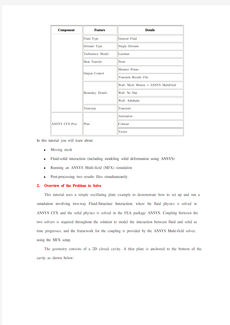
In this tutorial you will learn about:
?Moving mesh
?Fluid-solid interaction (including modeling solid deformation using ANSYS)
?Running an ANSYS Multi-field (MFX) simulation
?Post-processing two results files simultaneously.
2.Overview of the Problem to Solve
This tutorial uses a simple oscillating plate example to demonstrate how to set up and run a simulation involving two-way Fluid-Structure Interaction, where the fluid physics is solved in ANSYS CFX and the solid physics is solved in the FEA package ANSYS. Coupling between the two solvers is required throughout the solution to model the interaction between fluid and solid as time progresses, and the framework for the coupling is provided by the ANSYS Multi-field solver, using the MFX setup.
The geometry consists of a 2D closed cavity. A thin plate is anchored to the bottom of the cavity as shown below:
An initial pressure of 100 Pa is applied to one side of the thin plate for 0.5 seconds in order to distort it. Once this pressure is released, the plate oscillates backwards and forwards as it attempts to regain its equilibrium (vertical) position. The surrounding fluid damps the oscillations, which therefore have an amplitude that decreases in time. The CFX Solver calculates how the fluid responds to the motion of the plate, and the ANSYS Solver calculates how the plate deforms as a result of both the initial applied pressure and the pressure resulting from the presence of the fluid. Coupling between the two solvers is required since the solid deformation affects the fluid solution, and the fluid solution affects the solid deformation.
The tutorial describes the setup and execution of the calculation including the setup of the solid physics in Simulation (within ANSYS Workbench) and the setup of the fluid physics and ANSYS Multi-field settings in ANSYS CFX-Pre. If you do not have ANSYS Workbench, then you can use the provided ANSYS input file to avoid the need for Simulation.
3.Setting up the Solid Physics in Simulation (ANSYS Workbench)
This section describes the step-by-step definition of the solid physics in Simulation within ANSYS Workbench that will result in the creation of an ANSYS input file OscillatingPlate.inp. If you prefer, you can instead use the provided OscillatingPlate.inp file and continue from Setting up the Fluid Physics and ANSYS Multi-field Settings in ANSYS CFX-Pre.
Creating a New Simulation
1.If required, launch ANSYS Workbench.
2.Click Empty Project. The Project page appears displaying an unsaved project.
3.Select File > Save or click Save button.
4.If required, set the path location to a different folder. The default location is your working
directory. However, if you have a specific folder that you want to use to store files created during this tutorial, change the path.
5.Under File name, type OscillatingPlate.
6.Click Save.
7.Under Link to Geometry File on the left hand task bar click Browse. Select the provided
file OscillatingPlate.agdb and click Open.
8.Make sure that OscillatingPlate.agdb is highlighted and click New simulation from the
left-hand taskbar.
Creating the Solid Material
1.When Simulation opens, expand Geometry in the project tree at the left hand side of the
Simulation window.
2.Select Solid, and in the Details view below, select Material.
https://www.doczj.com/doc/0818684312.html,e the arrow that appears next to the material name Structural Steel to select New
Material.
4.When the Engineering Data window opens, right-click New Material from the tree view
and rename it to Plate.
5.Enter 2.5e06 for Young's Modulus, 0.35 for Poisson's Ratio and 2550 for Density.
Note that the other properties are not used for this simulation, and that the units for these values are implied by the global units in Simulation.
6.Click the Simulation tab near the top of the Workbench window to return to the
simulation.
Basic Analysis Settings
The ANSYS Multi-field simulation is a transient mechanical analysis, with a timestep of 0.1 s and a time duration of 5 s.
1.Select New Analysis > Flexible Dynamic from the toolbar.
2.Select Analysis Settings from the tree view and in the Details view below, set Auto Time
Stepping to Off.
3.Set Time Step to 0.1.
4.Under Tabular Data at the bottom right of the window, set End Time to
5.0 for the
Steps = 1 setting.
Inserting Loads
Loads are applied to an FEA analysis as the equivalent of boundary conditions in ANSYS CFX. In this section, you will set a fixed support, a fluid-solid interface, and a pressure load. Fixed Support
The fixed support is required to hold the bottom of the thin plate in place.
1.Right-click Flexible Dynamic in the tree and select Insert> Fixed Support from the
shortcut menu.
2.Rotate the geometry using the Rotate button so that the bottom (low-y) face of the
solid is visible, then select Face and click the low-y face.
That face should be highlighted to indicate selection.
3.Ensure Fixed Support is selected in the Outline view, then, in the Details view, select
Geometry and click 1 Face to make the Apply button appear (if necessary). Click Apply to set the fixed support.
Fluid-Solid Interface
It is necessary to define the region in the solid that defines the interface between the fluid in CFX and the solid in ANSYS. Data is exchanged across this interface during the execution of the simulation.
1.Right-click Flexible Dynamic in the tree and select Insert > Fluid Solid Interface from
the shortcut menu.
https://www.doczj.com/doc/0818684312.html,ing the same face-selection procedure described earlier, select the three faces of the
geometry that form the interface between the solid and the fluid (low-x, high-y and high-x faces) by holding down
Pressure Load
The pressure load provides the initial additional pressure of 100 [Pa] for the first 0.5 seconds of the simulation. It is defined using a step function.
1.Right-click Flexible Dynamic in the tree and select Insert > Pressure from the shortcut
menu.
2.Select the low-x face for Geometry.
3.In the Details view, select Magnitude, and using the arrow that appears, select Tabular
(Time).
4.Under Tabular Data, set a pressure of 100 in the table row corresponding to a time of 0.
Note: The units for time and pressure in this table are the global units of [s]and [Pa], respectively.
5.You now need to add two new rows to the table. This can be done by typing the new time
and pressure data into the empty row at the bottom of the table, and Simulation will automatically re-order the table in order of time value. Enter a pressure of 100 for a time value of 0.499, and a pressure of 0 for a time value of 0.5.
This gives a step function for pressure that can be seen in the chart to the left of the table. Writing the ANSYS Input File
The Simulation settings are now complete. An ANSYS Multi-field run cannot be launched from within Simulation, so the Solve buttons cannot be used to obtain a solution.
1.Instead, highlight Solution in the tree, select Tools> Write ANSYS Input File and
choose to write the solution setup to the file OscillatingPlate.inp.
2.The mesh is automatically generated as part of this process. If you want to examine it,
select Mesh from the tree.
3.Save the Simulation database, use the tab near the top of the Workbench window to return
to the Oscillating Plate [Project] tab, and save the project itself.
4.Setting up the Fluid Physics and ANSYS Multi-field Settings in ANSYS CFX-Pre
This section describes the step-by-step definition of the flow physics and ANSYS Multi-field settings in ANSYS CFX-Pre.
Playing a Session File
If you want to skip past these instructions and to have ANSYS CFX-Pre set up the simulation automatically, you can select Session > Play Tutorial from the menu in ANSYS CFX-Pre, then run the session file: OscillatingPlate.pre. After you have played the session file as described in earlier tutorials under Playing the Session File and Starting ANSYS CFX-Solver Manager, proceed to Obtaining a Solution using ANSYS CFX-Solver Manager.
Creating a New Simulation
1.Start ANSYS CFX-Pre.
2.Select File > New Simulation.
3.Select General and click OK.
4.Select File > Save Simulation As.
5.Under File name, type OscillatingPlate.
6.Click Save.
Importing the Mesh
1.Right-click Mesh and select Import Mesh.
2.Select the provided mesh file, OscillatingPlate.gtm and click Open.
Note:The file that was just created in Simulation, OscillatingPlate.inp, will be used as an input file for the ANSYS Solver.
Setting the Simulation Type
A transient ANSYS Multi-field run executes as a series of timesteps. The Simulation Type tab is used both to enable an ANSYS Multi-field run and to specify the time-related settings for it (in the External Solver Coupling settings). The ANSYS input file is read by ANSYS CFX-Pre so that it knows which Fluid Solid Interfaces are available.
Once the timesteps and time duration are specified for the ANSYS Multi-field run (coupling run), ANSYS CFX automatically picks up these settings and it is not possible to set the timestep and time duration independently. Hence the only option available for Time Duration is Coupling Time Duration, and similarly for the related settings Time Step and Initial Time.
1. Click
Simulation Type .
2. Apply the following settings
3. Click OK .
Note :You may see a physics validation message related to the difference in the units used in ANSYS CFX-Pre and the units contained within the ANSYS input file. While it is important to review the units used in any simulation, you should be aware that, in this specific case, the message is not crucial as it is related to temperature units and there is no heat transfer in this case. Therefore, this specific tutorial will not be affected by the physics message.
Creating the Fluid
A custom fluid is created with user-specified properties.
1. Click Material .
2. Set the name of the new material to Fluid.
3. Apply the following settings
4.Click OK.
Creating the Domain
In order to allow the ANSYS Solver to communicate mesh displacements to the CFX Solver, mesh motion must be activated in CFX.
1.Right click Simulation in the Outline tree view and ensure that Automatic Default
Domain is selected. A domain named Default Domain should now appear under the Simulation branch.
2.Double click Default Domain and apply the following settings
3.Click OK.
Creating the Boundary Conditions
In addition to the symmetry conditions, another type of boundary condition corresponding with the interaction between the solid and the fluid is required in this tutorial.
Fluid Solid External Boundary
The interface between ANSYS and CFX is defined as an external boundary in CFX that has its mesh displacement being defined by the ANSYS Multi-field coupling process.
When an ANSYS Multi-field specification is being made in ANSYS CFX-Pre, it is necessary to provide the name and number of the matching Fluid Solid Interface that was created in Simulation. Since the interface number in Simulation was 1, the name in question is FSIN_1. (If the interface number had been 2, then the name would have been FSIN_2, and so on.)
On this boundary, CFX will send ANSYS the forces on the interface, and ANSYS will send back the total mesh displacement it calculates given the forces passed from CFX and the other defined loads.
1.Create a new boundary condition named Interface.
2.Apply the following settings
3.Click OK.
Symmetry Boundaries
Since a 2D representation of the flow field is being modeled (using a 3D mesh with one element thickness in the Z direction) symmetry boundaries will be created on the low and high Z 2D regions of the mesh.
1.Create a new boundary condition named Sym1.
2.Apply the following settings
3.Click OK.
4.Create a new boundary condition named Sym2.
5.Apply the following settings
6.Click OK.
Setting Initial Values
Since a transient simulation is being modeled, initial values are required for all variables.
1. Click
Global Initialization
. 2. Apply the following settings:
3. Click OK .
Setting Solver Control
Various ANSYS Multi-field settings are contained under Solver Control under the External Coupling tab. Most of these settings do not need to be changed for this simulation.
Within each timestep, a series of “coupling” or “stagger” iterations are performed to ensure that CFX, ANSYS and the data exchanged between the two solvers are all consistent. Within each stagger iteration, ANSYS and CFX both run once each, but which one runs first is a user-specifiable setting. In general, it is slightly more efficient to choose the solver that drives the simulation to run first. In this case, the simulation is being driven by the initial pressure applied in ANSYS, so ANSYS is set to solve before CFX within each stagger iteration.
1. Click Solver Control .
2. Apply the following settings:
3.Click OK.
Setting Output Control
This step sets up transient results files to be written at set intervals.
1.Click Output Control .
2.On the Trn Results tab, create a new transient result with the default name.
3.Apply the following settings to Transient Results 1:
4.Click the Monitor tab.
5.Select Monitor Options.
6.Under Monitor Points and Expressions:
7.Click Add new item and accept the default name.
8.Set Option to Cartesian Coordinates.
9.Set Output Variables List to Total Mesh Displacement X.
10.Set Cartesian Coordinates to [0, 1, 0].
11.Click OK.
Writing the Solver (.def) File
1.Click Write Solver File .
2.If the Physics Validation Summary dialog box appears, click Yes to proceed.
3.Apply the following settings
4.Ensure Start Solver Manager is selected and click Save.
5.If you are notified the file already exists, click Overwrite.
6.This file is provided in the tutorial directory and will exist in your working folder if you
have copied it there.
7.Quit ANSYS CFX-Pre, saving the simulation (.cfx) file at your discretion.
5.Obtaining a Solution using ANSYS CFX-Solver Manager
The execution of an ANSYS Multi-field simulation requires both the CFX and ANSYS solvers to be running and communicating with each other. ANSYS CFX-Solver Manager can be used to launch both solvers and to monitor the output from both.
1.Ensure the Define Run dialog box is displayed.
There is a new MultiField tab which contains settings specific for an ANSYS Multi-field simulation.
2.On the MultiField tab, check that the ANSYS input file location is correct (the location is
recorded in the definition file but may need to be changed if you have moved files around).
3.On UNIX systems, you may need to manually specify where the ANSYS installation is if
it is not in the default location. In this case, you must provide the path to the v110/ansys directory.
4.Click Start Run.
The run begins by some initial processing of the ANSYS Multi-field input which results in the creation of a file containing the necessary multi-field commands for ANSYS, and then the ANSYS Solver is started. The CFX Solver is then started in such a way that it knows how to communicate with the ANSYS Solver.
After the run is under way, two new plots appear in ANSYS CFX-Solver Manager:
ANSYS Field Solver (Structural) This plot is produced only when the solid physics is set to use large displacements or when other non-linear analyses are performed. It shows convergence of the ANSYS Solver. Full details of the quantities are described in the ANSYS user documentation. In general, the CRIT quantities are the convergence criteria for each relevant variable, and the L2 quantities represent the L2 Norm of the relevant variable. For convergence, the L2 Norm should be below the criteria. The x-axis of the plot is the cumulative iteration number for ANSYS, which does not correspond to either timesteps or stagger iterations. Several ANSYS iterations will be
performed for each timestep, depending on how quickly ANSYS converges. You will usually see a somewhat “spiky” plot, as each quantity will be unconverged at the start of each timestep, and then convergence will improve.
ANSYS Interface Loads (Structural)This plot shows the convergence for each quantity that is part of the data exchanged between the CFX and ANSYS Solvers. In this case, four lines appear, corresponding to two force components (FX and FY) and two displacement components (UX and UY). Since the analysis is 2D, FZ and UZ are not exchanged. Each quantity is converged when the plot shows a negative value. The x-axis of the plot corresponds to the cumulative number of stagger iterations (coupling iterations) and there are several of these for every timestep. Again, a spiky plot is expected as the quantities will not be converged at the start of a timestep.
The ANSYS out file is displayed in ANSYS CFX-Solver Manager as an extra tab. Similar to the CFX out file, this is a text file recording output from ANSYS as the solution progresses.
1.Click the User Points tab and watch how the top of the plate displaces as the solution
develops.
2.When the solvers have finished and ANSYS CFX-Solver Manager puts up a dialog box
to tell you this, click Yes to post-process the results.
3.If using Standalone Mode, quit ANSYS CFX-Solver Manager.
6.Viewing Results in ANSYS CFX-Post
For an ANSYS Multi-field run, both the CFX and ANSYS results files will be opened up in ANSYS CFX-Post by default if ANSYS CFX-Post is started from a finished run in ANSYS CFX-Solver Manager.
Plotting Results on the Solid
When ANSYS CFX-Post reads an ANSYS results file, all the ANSYS variables are available to plot on the solid, including stresses and strains. The mesh regions available for plots by default are limited to the full boundary of the solid, plus certain named regions which are automatically created when particular types of load are added in Simulation. For example, any Fluid Solid Interface will have a corresponding mesh region with a name such as FSIN 1. In this case, there is also a named region corresponding to the location of the fixed support, but in general pressure loads do not result in a named region.
You can add extra mesh regions for plotting by creating named selections in Simulation - see the Simulation product documentation for more details. Note that the named selection must have a name which contains only English letters, numbers and underscores for the named mesh region to be successfully created.
Note that when ANSYS CFX-Post loads an ANSYS results file, the true global range for each variable is not automatically calculated, as this would add a substantial amount of time onto how long it takes to load such a file (you can turn on this calculation using Edit > Options and using the Pre-calculate variable global ranges setting under CFX-Post> Files). When the global range is first used for plotting a variable, it is calculated as the range within the current timestep. As subsequent timesteps are loaded into ANSYS CFX-Post, the Global Range is extended each time variable values are found outside the previous Global Range.
1.Turn on the visibility of Boundary ANSYS (under ANSYS > Domain ANSYS).
2.Right-click a blank area in the viewer and select Predefined Camera > View Towards
-Z. Zoom into the plate to see it clearly.
3.Apply the following settings to Boundary ANSYS:
4.Click Apply.
5.Select Tools> Timestep Selector from the task bar to open the Timestep Selector
dialog box. Notice that a separate list of timesteps is available for each results file loaded, although for this case the lists are the same. By default, Sync Cases is set to By Time Value which means that each time you change the timestep for one results file, ANSYS CFX-Post will automatically load the results corresponding to the same time value for all other results files.
6.Set Match to Nearest Available.
7.Change to a time value of 1 [s] and click Apply.
The corresponding transient results are loaded and you can see the mesh move in both the CFX and ANSYS regions.
1.Clear the visibility check box of Boundary ANSYS.
2.Create a contour plot, set Locations to Boundary ANSYS and Sym2, and set Variable to
Total Mesh Displacement. Click Apply.
https://www.doczj.com/doc/0818684312.html,ing the timestep selector, load time value 1.1 [s] (which is where the maximum total
mesh displacement occurs).
This verifies that the contours of Total Mesh Displacement are continuous through both the ANSYS and CFX regions.
Many FSI cases will have only relatively small mesh displacements, which can make visualization of the mesh displacement difficult. ANSYS CFX-Post allows you to visually magnify the mesh deformation for ease of viewing such displacements. Although it is not strictly necessary for this case, which has mesh displacements which are easily visible unmagnified, this is illustrated by the next few instructions.
https://www.doczj.com/doc/0818684312.html,ing the timestep selector, load time value 0.1 [s] (which has a much smaller mesh
displacement than the currently loaded timestep).
2.Place the mouse over somewhere in the viewer where the background color is showing.
Right-click and select Deformation > Auto. Notice that the mesh displacements are now exaggerated. The Auto setting is calculated to make the largest mesh displacement a fixed percentage of the domain size.
3.To return the deformations to their true scale, right-click and select Deformation > True
Scale.
Creating an Animation
https://www.doczj.com/doc/0818684312.html,ing the Timestep Selector dialog box, ensure the time value of 0.1 [s] is loaded.
2.Clear the visibility check box of Contour 1.
3.Turn on the visibility of Sym2.
4.Apply the following settings to Sym2.
5.Click Apply.
6.Create a vector plot, set Locations to Sym1 and leave Variable set to Velocity. Set
Color to be Constant and choose black. Click Apply.
7.Select the visibility check box of Boundary ANSYS, and set Color to a constant blue.
8.Click Animation .
The Animation dialog box appears.
9.Select Keyframe Animation.
10.In the Animation dialog box:
a.Click New to create KeyframeNo1.
b.Highlight KeyframeNo1, then change # of Frames to 48.
c.Load the last timestep (50) using the timestep selector.
d.Click New to create KeyframeNo2.
The # of Frames parameter has no effect for the last keyframe, so leave it at the
default value.
e.Select Save MPEG.
f.Click Browse next to the MPEG file data box to set a path and file name for
the MPEG file.
If the file path is not given, the file will be saved in the directory from which
ANSYS CFX-Post was launched.
g.Click Save.
The MPEG file name (including path) will be set, but the MPEG will not be
created yet.
h.Frame 1 is not loaded (The loaded frame is shown in the middle of the
Animation dialog box, beside F:). Click To Beginning to load it then wait
a few seconds for the frame to load.
i.Click Play the animation .
The MPEG will be created as the animation proceeds. This will be slow, since a
timestep must be loaded and objects must be created for each frame. To view the
MPEG file, you need to use a viewer that supports the MPEG format.
11.When you have finished, exit ANSYS CFX-Post.
ANSYS流固耦合计算实例 Oscillating Plate with Two-Way Fluid-Structure Interaction Introduction This tutorial includes: , Features , Overview of the Problem to Solve , Setting up the Solid Physics in Simulation (ANSYS Workbench) , Setting up the Fluid Physics and ANSYS Multi-field Settings in ANSYS CFX-Pre , Obtaining a Solution using ANSYS CFX-Solver Manager , Viewing Results in ANSYS CFX-Post If this is the first tutorial you are working with, it is important to review the following topics before beginning: , Setting the Working Directory , Changing the Display Colors Unless you plan on running a session file, you should copy the sample files used in this tutorial from the installation folder for your software (
Oscillating Plate with Two-Way Fluid-Structure Interaction Introduction This tutorial includes: ?Features ?Overview of the Problem to Solve ?Setting up the Solid Physics in Simulation (ANSYS Workbench) ?Setting up the Fluid Physics and ANSYS Multi-field Settings in ANSYS CFX-Pre ?Obtaining a Solution using ANSYS CFX-Solver Manager ?Viewing Results in ANSYS CFX-Post If this is the first tutorial you are working with, it is important to review the following topics before beginning: ?Setting the Working Directory ?Changing the Display Colors Unless you plan on running a session file, you should copy the sample files used in this tutorial from the installation folder for your software (
CAE联盟论坛精品讲座系列 基于MpCCI的Abaqus和Fluent流固耦合案例 主讲人:mafuyin CAE联盟论坛总监 摘要:通过MpCCI流固耦合接口程序,对某薄壁管道流动中的传热过程进行了Abaqus和Fluent相结合的流固耦合仿真分析。信息介绍了从建模、设置到求解计算和后处理的全过程,对相关研究人员具有参考意义。 1 分析模型 用三维建模软件solidworks建立了一个管径为1m的弯管,结构尺寸如图1a所示,管的结构如图1b所示,流体的模型如图1c所示。值得注意的是,由于拓扑特征的原因,这样的管壁模型无法通过对圆环扫略直接生成,而需先通过对大圆的扫略生成实心的模型(类似于流体模型),然后进行抽壳得到管壁的模型。用同样的方法对大圆半径减去管壁厚度的圆进行扫略得到流体模型。 a. 尺寸关系 b. 管壁结构 c. 流体模型 图1. 几何模型示意图 图2. 流固耦合传热分析模型示意图 内壁面(耦合面) 速度入口 v=6m/s; T in=600K 外壁面 压力出口 P=0Pa;T out=300K
由于管壁结构和流体的热学行为不同,传热系数等都不一样,所以属于典型的流固耦合传热问题,热学模型如图2所示。即管的一端为流体速度入口,一端为压力出口,给定流体外壁面一个初始温度600K,流体入口速度为6m/s,温度为600K,出口相对大气压力为0Pa,出口温度为300K。需要求解流体和管壁的温度场分布情况。 2 流体模型 将图1c的流体模型以Step格式导入Fluent软件通常使用的前处理器Gambit中,如图3a所示。设置求解器为,然后划分体网格,网格尺寸为100mm,类型为六面体单元,一共生成4895个体单元,网格如图3b所示。 a. 导入Gambit软件中的流体模型 b. 流场的网格模型 图3. 流体模型及网格示意图 进行网格划分后,需定义边界条件,在Gambit软件中先分别定义速度入口(VELOCITY_INLET)、压力出口(PRESSURE_OUTLET)和壁面(Wall)三组边界条件,具体参数设置在Fluent软件中进行。然后定义流体属性,名称定义为air,类型为Fluid。这些定义的目的是能够在Fluent软件中识别出这些特征,具体类型和参数都可以在Fluent软件中进行设置和修改。定义完后点击【Export】,选择【Mesh】,选择路径和文件名称并进行输出。 打开Fluent6.3.26或以上的版本,选择3D求解器,点击【File】→【Read】→【Case】,然后选择Gambit中输出的msh文件,即可将网格文件读入Fluent 软件中。读入模型后,进行求解参数和条件的设置。
基于MpCCI 的Abaqus 和Fluent 流固耦合案例 mafuyin 摘要:通过MpCCI 流固耦合接口程序,对某薄壁管道流动中的传热过程进行了Abaqus 和Fluent 相结合的流固耦合仿真分析。信息介绍了从建模、设置到求解计算和后处理的全过程,对相关研究人员具有参考意义。 1 分析模型 用三维建模软件solidworks 建立了一个管径为1m 的弯管,结构尺寸如图1a 所示,管的结构如图1b 所示,流体的模型如图1c 所示。值得注意的是,由于拓扑特征的原因,这样的管壁模型无法通过对圆环扫略直接生成,而需先通过对大圆的扫略生成实心的模型(类似于流体模型),然后进行抽壳得到管壁的模型。用同样的方法对大圆半径减去管壁厚度的圆进行扫略得到流体模型。 a. 尺寸关系 b. 管壁结构 c. 流体模型 图1. 几何模型示意图 图2. 流固耦合传热分析模型示意图 内壁面(耦合面) 速度入口 v=6m/s; T in =600K 外壁面 压力出口 P=0Pa ;T out =300K
由于管壁结构和流体的热学行为不同,传热系数等都不一样,所以属于典型的流固耦合传热问题,热学模型如图2所示。即管的一端为流体速度入口,一端为压力出口,给定流体外壁面一个初始温度600K,流体入口速度为6m/s,温度为600K,出口相对大气压力为0Pa,出口温度为300K。需要求解流体和管壁的温度场分布情况。 2 流体模型 将图1c的流体模型以Step格式导入Fluent软件通常使用的前处理器Gambit 中,如图3a所示。设置求解器为,然后划分体网格,网格尺寸为100mm,类型为六面体单元,一共生成4895个体单元,网格如图3b所示。 a. 导入Gambit软件中的流体模型 b. 流场的网格模型 图3. 流体模型及网格示意图 进行网格划分后,需定义边界条件,在Gambit软件中先分别定义速度入口(VELOCITY_INLET)、压力出口(PRESSURE_OUTLET)和壁面(Wall)三组边界条件,具体参数设置在Fluent软件中进行。然后定义流体属性,名称定义为air,类型为Fluid。这些定义的目的是能够在Fluent软件中识别出这些特征,具体类型和参数都可以在Fluent软件中进行设置和修改。定义完后点击【Export】,选择【Mesh】,选择路径和文件名称并进行输出。 打开Fluent6.3.26或以上的版本,选择3D求解器,点击【File】→【Read】→【Case】,然后选择Gambit中输出的msh文件,即可将网格文件读入Fluent 软件中。读入模型后,进行求解参数和条件的设置。 (1)模型缩放:为了便于分析结果数据特征,统一采用国际单位制进行仿真,
Ansys14 workbench血管流固耦合实例 根据收集的一些资料,进行学习后,试着做了这个ansys14workbench的血管流固耦合模拟,感觉能够耦合上,仅是熟悉流固耦合分析过程,不一定正确,仅供参考,希望大家多讨论。谢谢! 1、先在proe5中建立血管与血液流体区的模型(两者装配起来),或者直接在workbench中建模。 图1 模型图 2、新建工程。在workbench中toolbox中选custom system,双击FSI: FluidFlow(fluent)->static structure. 图2 计算工程 3、修改engineering data,因为系统缺省材料是钢,需要构建血管材料,如图3所示。先复制steel,而后修改密度1150kg/m3,杨氏模量4.5e8Pa,泊松比0.3,重新命名,最后在主菜单中点击“update project”保存.
图3 修改工程材料 4、模型导入,进入gemetry模块,import外部模型文件。 图4 模型导入图 5、进入FLUENT网格划分。 在workbench工程视图中的Mesh上点击右键,选择Edit…,如图5所示,进入网格划分meshing界面,如图6所示。我们这里需要去掉血管部分,只保留血液几何。
图5 进入网格划分
图6 禁用血管模型 6、设置网格方法。 默认是采用ICEM CFD进行网格划分,设置方式如图7所示,截面圆弧边分为12份,纵截面的边均分为10份,网格结果如图8所示。另外在这个界面中要设置边界的几何面,如inlet、outlet、symmetry 图7 设置网格划分方式 图8 最终出网格
new config fluid title 基于流固耦合作用下的双龙富水隧道稳定性研宄 set fluid off set log on set logfile yang 1 .log genzonradcylpOOOOpl 9.00 0p2 0 50 0 p3 0 0 8 size4 20 64 dim6 5 6 5 rat 1 1 I 1 group 围岩 gen zon cshell pOOOOpl 6.0 0 0 p2 0 50 0 p3 0 0 5.0 size 4 2064 dim 5.6 4.6 5.6 4.6 rat 1 1 1 1 group初期支护 gen zon cshell pO 0 0 0 pi 5.6 0 0 p2 0 50 0 p3 0 0 4.6 size 4 2064 dim 5.0 4.0 5.0 4.0 rat 1 1 1 1 group 二次衬砲fill group原岩 gen zon radcyl pOOOOpl 0 0 ?8.0 p2 0 50 0 p3 9.0 0 0 size 4 20 64 dim 3 6 3 6 rat 1 1 1 1 group围岩2 gen zon cshell pOOO Opl 0 0 -3.0 p2 0 50 0 p3 6.0 0 0 size 4 2064 dim 2.6 5.6 2.6 5.6 rat 1 1 1 1 group仰拱初期支护 gen zon cshell pO 0 0 Opl 0 0 -2.6 p2 0 50 0 p3 5.6 0 0 size 4 2064 dim2 5 2 5 rat 1 1 1 1 group仰拱二次衬砲fill group仰拱原岩 gen zone reflect normal -10 0 gen zone radtun pO 0 0 0 pi 45 0 0 p2 0 50 0 p3 0 0 20 size 3 20 3 12 dim 9 8 9 8 rat 1 1 1 1.1 group围岩3 gen zon reflect dip 0 ori 0 0 0 range x09y0 50z8 20 gen zon reflect dip 0 ori 0 0 0 range x 9 45 y 0 50 z 0 20 gen zon reflect dip 90 dd 270 ori 0 0 0 range x09y0 50z8 20 gen zon reflect dip 90 dd 270 ori 0 0 0 range x 0 9 y 0 50 z -8 -20 gen zon reflect dip 90 dd 270 ori 0 0 0 range x 9 45 y 0 50 z -20 20 save shuitun一model.sav model fl_iso prop perm 1.23e-9 poro 0.45 range z 4.5 20 prop perm 4.70e-10 poro 0.4 range z -20 4.5 set fl biot off ini fdensity le3 ini sat 1.0 ini food 2.0e9 ftens -le-3 ;假设围岩岩体符合mohr-coulomb本构模型,给围岩陚参数命令流如下, ;mohr-coulomb model model mohr def derive s_modl=E一modl/(2.0*(l .0+p—ratio 1)) b_modl=E_modl/(3.0*(1.0-2.0*p_ratiol)) s_mod2=E—mod2/(2.0*(l .0+p_ratio2)) bjmod2~E_mod2/(3.0*( 1.0-2.0*p_ratio2)) end
一般说来,ANSYS的流固耦合主要有4种方式: 1,sequential 这需要用户进行APDL编程进行流固耦合 sequentia指的是顺序耦合 以采用MpCCI为例,你可以利用ANSYS和一个第三方CFD产品执行流固耦合分析。在这个方法中,基于网格的平行代码耦合界面(MpCCI) 将ANSYS和CFD程序耦合起来。即使网格上存在差别,MpCCI也能够实现流固界面的数据转换。ANSYS CD中包含有MpCCI库和一个相关实例。关于该方法的详细信息,参见ANSYS Coupled-Field Analysis Guide中的Sequential Couplin 2,FSI solver 流固耦合的设置过程非常简单,推荐你使用这种方式 3,multi-field solver 这是FSI solver的扩展,你可以使用它实现流体,结构,热,电磁等的耦合 4,直接采用特殊的单元进行直接耦合,耦合计算直接发生在单元刚度矩阵 一个流固耦合的例子 length=2 width=3 height=2 /prep7 et,1,63 et,2,30 !选用FLUID30单元,用于流固耦合问题 r,1,0.01 mp,ex,1,2e11 mp,nuxy,1,0.3 mp,dens,1,7800 mp,dens,2,1000 !定义Acoustics材料来描述流体材料-水 mp,sonc,2,1400 mp,mu,0, ! block,,length,,width,,height esize,0.5 mshkey,1 ! type,1 mat,1 real,1 asel,u,loc,y,width amesh,all alls ! type,2 mat,2 vmesh,all
有问题可以发邮件给我一起讨论xw4996@https://www.doczj.com/doc/0818684312.html, FSI流固耦合命令求解流固耦合问题 使用ANSYS计算结构在水中的模态时, FLUID29,FLUID30单元分别用来模拟二维和三维流体部分,相应的结构模型则利用PLANE42单元和SOL ID45等单元来构造,其中,PLANE42和SOL ID45分别是用来构造二维和三维结构模型的单元。FLUID30是流体声单元,主要用于模拟流体介质及流固耦合问题。该单元有8 个节点,每个节点上有4 个自由度,分别是XYZ上3个方向位移自由度和1个压力自由度,为各向同性材料。输入材料属性时,需要输入流体的材料密度(作为DENS 输入)及流体声速(作为SONC输入),流体粘性产生的损耗效应忽略不计。FLUID29是FLUID30单元在二维上的简化,少了一个Z向的位移。SOLID45单元用于构造三维实体结构。单元通过8 个节点来定义,每个节点有 3 个沿着XYZ方向平移的自由度。PLANE42是SOLID45单元在二维上的简化。 在利用ANSYS建模分析时,流场域单元属性分为2种,由KEYOPT(2)(指定流体和结构分界面处结构是否存在) 控制,在流固耦合交界面上的单元KEYOPT(2) = 0 ,表示分界面处有结构,其他流体单元KEYOPT(2)=1,表示分界面处无结构。流体-结构分界面通过面载荷标志出来,指定FSI label可以把分界面处的结构运动和流体压力耦合起来,分界面标志在分界面处的流体单元标出。 数值分析的步骤 1) 建立流体单元的实体模型。建立流体模型,需要确定流体域的范围,可以把无限边界流体简化成流体区域的半径为固体结构半径的10倍。 2) 标记流固耦合界面。选取流体单元中流固交界面上的节点,执行FSI 命令,流固耦合交界面的处理:流体与固体是两个独立的实体,在划分单元时在两者交界面上的单元网格要划分一致,这样在交界面上的同一位置一般就有两个重合的节点,一个节点属于流体单元,一个节点属于固体单元,这两个重合节点在交界面的位移强制保持一致。 3) 建立固体结构实体模型。建立固体结构模型,定义单元属性,采用映射方式进行网格的划分。 4) 施加约束条件。由于流体区域的尺寸远大于固体结构尺寸,故可以不考虑流体液面的重力的影响,将流体边界处的单元节点上施加压力(PRES) 为零的约束。因为选择的算例为悬臂结构,在固体结构底部加全约束。 5) 选择求解算法,进行求解。定义分析类型为模态分析,设定提取频率阶数和提取模态的方法。因为耦合问题的刚度矩阵,质量矩阵都不对称,需要采用非对称矩阵法(UNSYMMETRIC)求解。 6) 查看结果。进入后处理模块,查看结构模型的频率及振型。 以半浸没与水中的桥墩模态问题为背景,并假设: 1. 桥墩为实心等截面的实体,实际桥墩模型应该是空心壳体,截面尺寸也 非常复杂,因而需要分块划分单元。
说明:本例只应用于FLUENT14.0以上版本。 ANSYS 14.0是2011年底新推出的版本,在该版本中,加入了一个新的模块System Coupling,目前只能用于fluent与ansys mechanical的双向流固耦合计算。官方文档中有介绍说以后会逐渐添加对其它求解器的支持,不过这不重要,重要的是现在FLUENT终于可以不用借助第三方软件进行双向流固耦合计算了,个人认为这是新版本一个不小的改进。 模块及数据传递方式如下图所示。 一、几何准备 流固耦合计算的模型准备与单独的流体计算不同,它需要同时创建流体模型与固体模型。在geometry模块中同时创建流体模型与固体模型。到后面流体模型或固体模块中再进行模型禁用处理。 模型中的尺寸:v1:32mm,h2:120mm,h5:60mm,h3:3mm,v4:15mm。
由于流体计算中需要进行动网格设置,因此推荐使用四面体网格。当然如果挡板刚度很大网格变形很小时,可以使用六面体网格,划分六面体网格可以先将几何进行slice切割。这里对流体区域网格划分六面体网格,固体域同样划分六面体网格。 二、流体部分设置 1、网格划分 双击B3单元格,进入meshing模块进行网格划分。禁用固体部分几何。设定各相关部分的尺寸,由于固体区域几何较为整齐,因此在切割后只需设定一个全局尺寸即可划分全六面体网格。这里设定全局尺寸为1mm。划分网格后如下图所示。 2、进行边界命名,以方便在fluent中进行边界条件设置 设置左侧面为速度进口velocity inlet,右侧面为自由出流outflow,上侧面为壁面边界wall_top,正对的两侧面为壁面边界wall_side1与wall_side2(这两个边界在动网格设定中为变形域),设定与固体交界面为壁面边界(该边界在动网格中设定为system coupling类型)。 操作方式:选择对应的表面,点击右键,选择菜单create named selection,然后输入相应的边界名称。注意:FLUENT会自动检测输入的名称以使用对应的边界类型,当然用户也可以在fluent进行类型更改。完成后的树形菜单如下图所示。
双向流固耦合实例(Fluent与structure) 说明:本例只应用于FLUENT14.0以上版本。 ANSYS 14.0是2011年底新推出的版本,在该版本中,加入了一个新的模块System Coupling,目前只能用于fluent与ansys mechanical的双向流固耦合计算。官方文档中有介绍说以后会逐渐添加对其它求解器的支持,不过这不重要,重要的是现在FLUENT终于可以不用借助第三方软件进行双向流固耦合计算了,个人认为这是新版本一个不小的改进。 模块及数据传递方式如下图所示。 一、几何准备 流固耦合计算的模型准备与单独的流体计算不同,它需要同时创建流体模型与固体模型。在geometry模块中同时创建流体模型与固体模型。到后面流体模型或固体模块中再进行模型禁用处理。 模型中的尺寸:v1:32mm,h2:120mm,h5:60mm,h3:3mm,v4:15mm。 由于流体计算中需要进行动网格设置,因此推荐使用四面体网格。当然如果挡板刚度很大网格变形很小时,可以使用六面体网格,划分六面体网格可以先将几何进行slice切割。这里对流体区域网格划分六面体网格,固体域同样划分六面体网格。 二、流体部分设置 1、网格划分 双击B3单元格,进入meshing模块进行网格划分。禁用固体部分几何。设定各相关部分的尺寸,由于固体区域几何较为整齐,因此在切割后只需设定一个全局尺寸即可划分全六面体网格。这里设定全局尺寸为1mm。划分网格后如下图所示。
2、进行边界命名,以方便在fluent中进行边界条件设置 设置左侧面为速度进口velocity inlet,右侧面为自由出流outflow,上侧面为壁面边界wall_top,正对的两侧面为壁面边界wall_side1与wall_side2(这两个边界在动网格设定中为变形域),设定与固体交界面为壁面边界(该边界在动网格中设定为system coupling类型)。 操作方式:选择对应的表面,点击右键,选择菜单create named selection,然后输入相应的边界名称。注意:FLUENT会自动检测输入的名称以使用对应的边界类型,当然用户也可以在fluent进行类型更改。完成后的树形菜单如下图所示。 本部分操作完毕后,关闭meshing模块。返回工程面板。 3、进入fluent设置 FLUENT主要进行动网格设置。其它设置与单独进行FLUENT仿真完全一致。 设置使用瞬态计算,使用K-Epsilon湍流模型。 这里的动网格主要使用弹簧光顺处理(由于使用的是六面体网格且运动不规律),需要使用TUI命令打开光顺对六面体网格的支持。使用命令 /define/dynamic-mesh/controls/smoothing-parameters。 动态层技术与网格重构方法在六面体网格中失效。因此,建议使用四面体网格。我们这里由于变形小,所以只使用光顺方法即可满足要求。 点击Dynamic mesh进入动网格设置面板。如下图所示,激活动网格模型。
例子的来源是Abaqus CLE的官方教程,可是写的太粗线条,我还是搞了两天才做 出了这个例子。其实就是个滚筒洗衣机带着洗衣机里的水一起转的问题。 1. 分别为Eulerian domain和Lagrangian domain建立两个part 建立Lagrangian domain的Part,类型设置为Discrete rigid,并设置Reference Point。 建立Eulerian domain的Part,类型设置为Eulerian,要注意Eulerian domain 和Lagrangian domain要保证有重叠的部分,这是一种弱耦合,数据在两个区域间抛来抛去,所以网格要有重叠部分。这导致在Eulerian domain里有的部分是有材料的,有的地方是没有材料的。为了之后设置材料分布时候方便,要把part实现划出几个辅助的partition。黄色虚线是在划分partition时,为了指明 Extrude/Sweep方向用到的辅助坐标轴。
2. 定义水的材料属性 选择状态方程模型EOS中Us-Up,设置声速c0=1483m/s;密度为1000kg/m3;粘度为0.001kg/ms。并把截面属性赋给Eulerian domain。
3. 把两个Part组装起来
4. 新建一个Step-1 5. 为Eulerian domain和Lagrangian domain划分网格
6. 设置接触 新建一个Contact Property,因为不是普通的面和面的接触,水中的任何的一个部
分可能在流动区域里的任何一个地方和Lagrangian domain接触,设置Tangential Behavior为Rough,赋给水和洗衣机之间的关系。新建一个Interaction,把刚才的Contact Property赋给它。 更重要的是设置接触的两个Surface。其中一个Surface是Lagrangian domain 部分的内侧面,为Geometry类型,另一个Surface是Eulerian domain的全部网格,为Mesh类型。
达尔文档DareDoc 分享知识传播快乐 ANSYS流固耦合分析实例命令流 本资料来源于网络,仅供学习交流 2015年10月达尔文档|DareDoc整理
目录 ANSYS流固耦合例子命令流.......................................................................... 错误!未定义书签。ANSYS流固耦合的方式 (3) 一个流固耦合模态分析的例子1 (3) 一个流固耦合模态分析的例子2 (4) 一个流固耦合建模的例子 (7) 一加筋板在水中的模态分析 (8) 一圆环在水中的模态分析 (10) 接触分析实例---包含初始间隙 (14) 耦合小程序 (19) 流固耦合练习 (21) 一个流固耦合的例子 (22) 使用物理环境法进行流固耦合的实例及讲解 (23) 针对液面晃动问题,ANSYS/LS-DYNA提供三种方法 (30) 1、流固耦合 (30) 2、SPH算法 (34) 3、ALE(接触算法) (38) 脱硫塔于浆液耦合的分析 (42) ANSYS坝-库水流固耦合自振特性的例子 (47) 空库时的INP文件 (47) 满库时的INP文件 (49) 计算结果 (52)
ANSYS流固耦合的方式 一般说来,ANSYS的流固耦合主要有4种方式: 1,sequential 这需要用户进行APDL编程进行流固耦合 sequentia指的是顺序耦合 以采用MpCCI为例,你可以利用ANSYS和一个第三方CFD产品执行流固耦合分析。在这个方法中,基于网格的平行代码耦合界面(MpCCI) 将ANSYS和CFD程序耦合起来。即使网格上存在差别,MpCCI也能够实现流固界面的数据转换。ANSYS CD中包含有MpCCI库和一个相关实例。关于该方法的详细信息,参见ANSYS Coupled-Field Analysis Guide中的Sequential Couplin 2,FSI solver 流固耦合的设置过程非常简单,推荐你使用这种方式 3,multi-field solver 这是FSI solver的扩展,你可以使用它实现流体,结构,热,电磁等的耦合 4,直接采用特殊的单元进行直接耦合,耦合计算直接发生在单元刚度矩阵 一个流固耦合模态分析的例子1 这是一个流固耦合模态分析的典型事例,采用ANSYS/MECHANICAL可以完成。处理过程中需要注意以下几个方面的问题: 1、单元的选择; 2、流体材料模式; 3、流固耦合关系的定义; 4、模态提取方法。 length=2 width=3 height=2 /prep7 et,1,63 et,2,30 !选用FLUID30单元,用于流固耦合问题 r,1,0.01 mp,ex,1,2e11 mp,nuxy,1,0.3 mp,dens,1,7800 mp,dens,2,1000 !定义Acoustics材料来描述流体材料-水 mp,sonc,2,1400 mp,mu,0, ! block,,length,,width,,height esize,0.5 mshkey,1
length=2 !定义体各种变量参数,长宽高 width=3 height=2 /prep7 et,1,63 !选用壳模型 et,2,30 !选用FLUID30单元,用于流固耦合问题r,1,0.01 增加实常数,壳厚为0.01 mp,ex,1,2e11 mp,nuxy,1,0.3 mp,dens,1,7800 !定义壳单元的各种单元属性 mp,dens,2,1000 !定义Acoustics材料来描述流体材料-水mp,sonc,2,1400 !定义声单元声速 mp,mu,0, !定义吸声系数 ! block,,length,,width,,height !建立长方体 esize,0.5 mshkey,1 ! type,1 !选择壳单元 mat,1 real,1 asel,u,loc,y,width !选择面 amesh,all !划分面单元 alls !选择所有项 ! type,2 !选择声单元 mat,2 vmesh,all !划分体单元 fini /solu antype,2 modopt,unsym,10 !非对称模态提取方法处理流固耦合问题eqslv,front mxpand,10,,,1 nsel,s,loc,x, nsel,a,loc,x,length nsel,r,loc,y d,all,,,,,,ux,uy,uz, nsel,s,loc,y,width, d,all,pres,0 !上面几步为定义边界条件和约束 alls asel,u,loc,y,width, sfa,all,,fsi !定义流固耦合界面
alls !选择所有项 solv !求解 fini /post1 !后处理 set,first plnsol,u,sum,2,1 !显示图形 fini /PREP7 !定义壳材料与性质 !壳元素与材料 ET,1,shell63 $MP,EX,1,201E9 $MP,prxy,1,0.26 $MP,dens,1,7.85E3 $r,1,0.006 !流体元素与材料 ET,2,FLUID80 $MP,EX,2,1.5e9 $MP,DENS,2,0.84e3 $mp,visc,2,1.0e-10 !以下这个keyoption怎么用? 如过用1,就会显示[Element 877 may not have a positive Z coordinate IF KEYOPT(2) = 1.],显示这个错误代表要做什么修正吗?所以我暂时用KEYOPT(2) = 0就可以跑。 KEYOPT,2,2,0 !建立壳关键点 K,1,10,0,0 $K,2,10,0,12 !建立中心线关键点 k,3,0,0,0 $k,4,0,0,20 !定义壳壁线 L,1,2 $L,1,3 !以关键点3,4为中心线旋转360度生成壳体 AROTAT,all,,,,,,3,4,360 !划分壳体网格 AATT,1,1,1 $esize,2 $mshape,0,3D $mshkey,2 $amesh,all $alls !延伸出水位体积 VEXT,2,8,2,0,0,10,0,0,0 $vglue,all
ANSYS Workbench LS-DYNA流固耦合方法应用贮液容器(含塑料瓶)广泛应用于化工、食品包装、储运等领域。由于容器(含塑料瓶)在运输和使用过程中常常会因为跌落或碰撞冲击导致破损而造成损失和污染,因此,研究贮液容器(含塑料瓶)在跌落碰撞过程中的力学行为,对认识容器(含塑料瓶)跌落碰撞损伤机理,优化容器(含塑料瓶)结构,提高其安全性和使用价值意义重大。. 贮液容器的跌落是一个典型的流固耦合问题,可采用LS-DYNA的ALE算法(任意拉格朗日欧拉算法)进行模拟。下面以一个封闭的装水水箱为例,介绍ANSYS Workbench LS-DYNA 分析此类型跌落问题的方法和步骤: 1.建立几何模型 调用ANSYS Workbench中的LS-DYNA模块,如图1所示。然后使用ANSYS的CAD工具DesignModeler建立几何模型,如图2所示。 图1 调用Workbench LS-DYNA图2 DesignModeler中建立几何模型 2.生成K文件 双击进入“Model”后,对模型进行网格划分、边界条件设置、速度设置和分析设置,如图3所示。设置完成后点击“solve”求解,生成K文件,如图4所示。
图3调用Workbench LS-DYNA图4DesignModeler中建立几何模型 3.编辑K文件 通过Workbench LS-DYNA生成的K文件中关键字是不够完善的,并不能直接递交LS-DYNA求解器进行求解。K文件中所欠缺的一些关键字,在流固耦合分析中是必不可少的,如空材料的定义、跟随坐标系的定义、空白域的定义以及状态方程的定义等。 3.1重要关键字释义 (1)LS-DYNA程序提供了运动的多物质ALE网格,可以方便地为多物质ALE算法定义跟随坐标系 *ALE_REFERENCE_SYSTEM_NODE *ALE_REFERENCE_SYSTEM_GROUP (2)定义空材料和状态方程的关键字 *MAT_NULL*EOS (3)初始化空白域的关键字 *INITIAL_VOID_PART (4)结构和流体之间耦合的关键字 *CONSTRAINED_LAGRANGE_IN_SOLID (5)单元算法定义(单点积分的单物质加空白材料)的关键字 *SECTION_SOLID_ALE ELF0RM=12
实例3 隧道内具有柔性结构的流固耦合分析 问题:隧道内具有柔性结构的流固耦合如图3-1所示。 图3-1 流体-固体结构示意图 一、目的 1. 掌握流固耦合作用FSI在Adina-AUI中的操作过程。 2. 掌握用伸缩比例因子画流固耦合模型。 3. 定义引导点(leader-follower points)。 二、定义模型主控数据 1. 定义标题: 选Control→Heading→敲入标题“exe03: Fluid flow over a flexible structure in a channel, ADINA input”→and click OK。 2. FSI分析: 在右边Analysis Type区选FSI按钮。 3. 主控自由度 选Control→Degrees of Freedom→不选X-Translation, X-Rotation, Y-Rotation and Z-Rotation按钮→and click OK。 4. 分析假设:大位移,小应变。 选Control→Analysis Assumptions→Kinematics→设置“Displacements/Rotations”为 Large→ click OK。(注:非常薄的结构,因此为小应变)。
三、力学模型 1. 柔性结构建立模型 1). 柔性结构几何模型 坐标点如表3-1,几何结构如图3-2所示。 其几何面见表3-2所示。 ①选Define Points 图标→按表3-1输入几何点坐标→ click OK . ②选Define Surfaces 图标→设置TYPE 为Vertex → click OK(如图3-2所示)。 2). 施加固定边界条件和流- 固边界条件 ①. 图3-2中,在L2线上施加固定约束,其过程可用Adina-AUI 完成。 ②. 流-固边界,选Model →Boundary Conditions →FSI Boundary →add FSI boundary number 1→在表中头两行敲入流固边界线编号1和 3 and click OK 。 3). 定义材料特性 弹性模量1.0×10⁶(dyne/cm 2),泊松比0.3。(线弹性问题) 选Model →Materials →Elastic_Isotropic →add material 1, 设置弹性模量1.0E6→泊松比 0.3 and click OK . 4).定义单元和单元划分 (1). 2-D 实体单元,此问题属平面应变问题。 Element group : 选 Meshing →Element Groups → 增加单元组号 1→ 设置 the Type to 2-D Solid →设置 the Element 柔性结构 图3-2 几何模型 表3-1 模型几何点坐标 几何点 X1 X2 X3 坐标系 1 30.025 15.0 0 2 30.0 0.0 0 3 30.05 0.0 图3-3 结构网格
基于 LS-DYNA 及 FLUENT 的板壳结构流-固耦合分析
汪丽军
北京航空航天大学,交通科学与工程学院 100191
[摘 要]: 本文采用 ANSYS 显示动力分析模块 LS-DYNA 及流场分析模块 FLUENT,对水下的板壳 结构运动及其界面的流-固耦合现象进行了仿真分析。流场计算得到的界面压强数据以外载荷 的形式施加于结构表面,使其产生位移及变形;同时,结构的变化又进一步影响了流场的分 布。通过往复的双向耦合迭代,得到了板壳结构的动力学响应以及流场的分布情况。仿真结 果与试验结果的对比表明,此方法适用于解决兼有大位移及较大变形特征的流-固耦合问题。
[关键词]: 板壳结构 流-固耦合 有限元方法 ANSYS
Analysis of Fluid-Structure Interaction for Plate/Shell Structure Based on LS-DYNA and FLUENT
Wang Lijun School of Transportation Science & Engineering, Beihang University 100191
Abstract: In this paper,the movement of plate under water and the fluid-structure interaction(FSI) is simulated numerically by combining explicit dynamic solver LS-DYNA and computational fluid dynamics solver FLUENT in ANSYS. The pressure obtained from the calculation of flow field are applied as external loads on the surface of the plate, then the structural deformation and displacement can be calculated as well, which will affect the shape and pressure distribution of the flow field reversely. After sequential coupling iterations the dynamic response of the structure and flow field distribution are obtained consequently. By comparing numerical and experimental results it is proved that this proposed coupling method is suitable for solving such a kind of FSI problems considering both large displacement and comparatively large deformation.
Keyword: Plate/shell structure, Fluid-Structure Interaction, Finite element method,ANSYS
1 前言
在自然界中,流-固耦合现象广泛存在于航空、航天、汽车、水利、石油、化工、海洋 以及生物等领域。很多实际问题中流体载荷对于结构的影响不可忽略;同时,结构的位移 和变形也会对流场的分布产生重要影响。例如各种水下运动机构都需要考虑这种现象。