On the distribution of imaginary parts of zeros of the Riemann zeta function

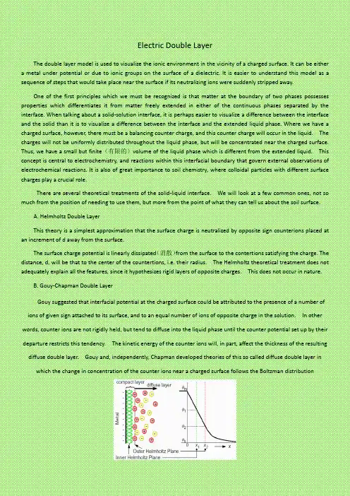
Electric Double LayerThe double layer model is used to visualize the ionic environment in the vicinity of a charged surface. It can be either a metal under potential or due to ionic groups on the surface of a dielectric. It is easier to understand this model as a sequence of steps that would take place near the surface if its neutralizing ions were suddenly stripped away.One of the first principles which we must be recognized is that matter at the boundary of two phases possesses properties which differentiates it from matter freely extended in either of the continuous phases separated by the interface. When talking about a solid-solution interface, it is perhaps easier to visualize a difference between the interface and the solid than it is to visualize a difference between the interface and the extended liquid phase. Where we have a charged surface, however, there must be a balancing counter charge, and this counter charge will occur in the liquid. The charges will not be uniformly distributed throughout the liquid phase, but will be concentrated near the charged surface. Thus, we have a small but finite（有限的）volume of the liquid phase which is different from the extended liquid. This concept is central to electrochemistry, and reactions within this interfacial boundary that govern external observations of electrochemical reactions. It is also of great importance to soil chemistry, where colloidal particles with different surface charges play a crucial role.There are several theoretical treatments of the solid-liquid interface. We will look at a few common ones, not so much from the position of needing to use them, but more from the point of what they can tell us about the soil surface.A. Helmholtz Double LayerThis theory is a simplest approximation that the surface charge is neutralized by opposite sign counterions placed at an increment of d away from the surface.The surface charge potential is linearly dissipated（消散）from the surface to the contertions satisfying the charge. The distance, d, will be that to the center of the countertions, i.e. their radius. The Helmholtz theoretical treatment does not adequately explain all the features, since it hypothesizes rigid layers of opposite charges. This does not occur in nature.B. Gouy-Chapman Double LayerGouy suggested that interfacial potential at the charged surface could be attributed to the presence of a number ofions of given sign attached to its surface, and to an equal number of ions of opposite charge in the solution. In otherwords, counter ions are not rigidly held, but tend to diffuse into the liquid phase until the counter potential set up by theirdeparture restricts this tendency. The kinetic energy of the counter ions will, in part, affect the thickness of the resultingdiffuse double layer. Gouy and, independently, Chapman developed theories of this so called diffuse double layer inwhich the change in concentration of the counter ions near a charged surface follows the Boltzman distributionn = n o exp(-zeY/kT)where n o= bulk concentrationz = charge on the ione = charge on a protonk = boltzman constantAlready, however, we are in error, since derivation（起源）of this form of the Boltzman distribution assumes that activity is equal to molar concentration. This may be an OK approximation for the bulk solution, but will not be true near a charged surface.Now, since we have a diffuse double layer, rather than a rigid double layer, we must concern ourselves with the volume charge density rather than surface charge density when studying the coulombic interactions between charges. The volume charge density, r, of any volume, i, can be expressed asr i = Sz i en iThe coulombic interaction between charges can, then, be expressed by the Poisson equation. For plane surfaces, this can be expressed asd2Y/dx2 = -4pr/dwhere Y varies from Y o at the surface to 0 in bulk solution. Thus, we can relate the charge density at any given point to the potential gradient away from the surface.Combining the Boltzmann distribution with the Poisson equation and integrating under appropriate limits, yields the electric potential as a function of distance from the surface. The thickness of the diffuse double layer:l double = [erkT/(4pe2Sn i oz i2)]1/2at room temperature can be simplified asl double = 3.3*106er/(zc1/2)in other words, the double layer thickness decreases with increasing valence and concentration.The Gouy-Chapman theory describes a rigid charged surface, with a cloud of oppositely charged ions in the solution, the concentration of the oppositely charged ions decreasing with distance from the surface. This is the so-called diffuse double layer.This theory is still not entirely accurate. Experimentally, the double layer thickness is generally found to be somewhat greater than calculated. This may relate to the error incorporated in assuming activity equals molar concentration when using the desired form of the Boltzman distribution. Conceptually, it tends to be a function of the fact that both anions and cations exist in the solution and with increasing distance away from the surface the probability that ions of the same sign as the surface charge will be found within the double layer increase as well.C. Stern Modification of the Diffuse double LayerThe Gouy-Chapman theory provides a better approximation of reality than does the Helmholtz theory, but it still has limited quantitative application. It assumes that ions behave as point charges, which they cannot, and it assumes that there is no physical limits for the ions in their approach to the surface, which is not true. Stern, therefore, modified the Gouy-Chapman diffuse double layer. His theory states that ions do have finite size so cannot approach the surface closer than a few nm. The first ions of the Gouy-Chapman Diffuse Double Layer are not at the surface, but at some distance d away from the surface. This distance will usually be taken as the radius of the ion. As a result, the potential and concentration of the diffuse part of the layer is low enough to justify treating the ions as point charges.Stern also assumed that it is possible that some of the ions are specifically adsorbed by the surface in the plane d, and this layer has become known as the Stern Layer. Therefore, the potential will drop by Yo - Yd over the "molecular condenser" (ie. the Helmholtz Plane) and by Yd over the diffuse layer. Yd has become known as the zeta (z) potential.This diagram serves as a visual comparison of the amount of counterions in each the Stearn Layer and the Diffuse Layer of smectite when saturated with the three alkali earth ions, as in the above table.The double layer is formed in order to neutralize the charged surface and, in turn, causes an electrokinetic potential between the surface and any point in the mass of the suspending liquid. This voltage difference is on the order of millivolts （毫伏）and is referred to as the surface potential. The magnitude of the surface potential is related to the surface charge and the thickness of the double layer. As we leave the surface, the potential drops off roughly linearly in the Stern layer and then exponentially through the diffuse layer, approaching zero at the imaginary boundary of the double layer. The potential curve is useful because it indicates the strength of the electrical force between particles and the distance at which this force comes into play. A charged particle will move with a fixed velocity in a voltage field. This phenomenon is called electr ophoresis. The particle’s mobility is related to the dielectric constant and viscosity of the suspending liquid and to the electrical potential at the boundary between the moving particle and the liquid. This boundary is called the slip plane and is usually defined as the point where the Stern layer and the diffuse layer meet. The relationship between zeta potential and surface potential depends on the level of ions in the solution. The figure above represents the change in charge density through the diffuse layer. One shows considered to be rigidly attached to the colloid, while the diffuse layer is not. As a result, the electrical potential at this junction is related to the mobility of the particle and is called the zeta potential. Although zeta potential is an intermediate value, it is sometimes considered to be more significant than surface potential as far as electrostatic repusion is concerned.。

Multiplying S{s^ k) by N*{s) we obtain the following result. L e m m a 3.1 5(s, k) is Hurwitz if and only if ai{5{s,k)N*{s)) = n-{l{Nis))-r{N{s))). (3.2)
CONTROLLER
PLANT
FIGURE 3.1. Feedback control system. To this end, consider the feedback system shown in Fig. 3.1. Here r is the command signal, y is the output. G(s) = Njs)
then, (3.1) can be rewritten as 6{s, k) - [kNe{s^) + De{s^)] + s[kNo{s^) + Dois^)] .
3.2 A Characterization of All Stabilizing Feedback Gains
41
It is clear from this expression that both the even as well as the odd parts of 6{s, k) depend on k. This creates difficulties when trying to use Lemma 2.1 to ensure the Hurwitz stability of 5{s, k). To overcome this problem, we will now construct a polynomial for which only the even part depends on fc, and to which Theorem 2.4 is applicable. Suppose that the degree of D{s) is n while the degree of N{s) is m and m < n. Define iV*(5) : - N{-s) = Ne{s^) sNois^).

In-bund distortion: The new clip-and-filter technique causes no increase in out-of-band power so the limit to PAPR reduction in a practical system is the in-band distortion, in the form of clipping noise. A number of authors have analysed the effects of nonlinearities on OFDM signals [2]. The real and imaginary components of an OFDM signal have Gaussian distributions, thus by extending Bussgang’stheory to thecomplexcaseitispossibleto showthat, subjecttocertainconditions, [2]
J. Armstrong
It is shown that repeated clipping and frequency domain filtering of an orthogonal frequency division multiplexing (OFDM) signal can significantly reduce the peak-to-average power ratio (PAPR) of the transmitted signal. The technique causes no increase in out-of-band power. Significant PAPR reduction can be achieved with only moderate levels of clipping noise.

THE RIEMANN HYPOTHESISMICHAEL ATIYAH1.IntroductionIn my Abel lecture [1] at the ICM in Rio de Janeiro 2018, I explained how to solve a long-standing mathematical problem that had emerged from physics. The problem was to understand the fine structure constant α.The full details are contained in [2] which has been submitted to proceedings A of the Royal Society. The techniques developed in [2] are a novel fusion of ideas of von Neumann and Hirzebruch. They are sophisticated and powerful, based on an infinite iteration of exponentials, while having an inherent simplicity.Attacking the mystery of α was the motivation, but the power and universality of the methods indicated that they should solve other hard problems, or at least shed new light on them if they are insoluble. In expanding my Abel Lecture for the ICM Proceedings I speculated that the techniques of [2] might lead to the new subject of Arithmetic Physics.The Riemann Hypothesis RH is the assertion that ζ(s) has no zeros in the critical strip 0 < Re(s) < 1 , off the critical line Re(s) = 1/2. It is one of the most famous unsolved problems in mathematics and a formidable challenge for the programme envisaged in [1]. I believe it will live up to this challenge, and this paper will provide the proof.The proof depends on a new function T (s), the Todd function, named by Hirzebruch after my teacher J.A.Todd. Its definition and properties are all in [2] but, in section 2, I will review and clarify them. In section 3 I will use the function T (s) to prove RH. In section 4, entitled Deus ex Machina, I will try to explain the mystery of this simple proof of RH. Finally, in section 5, I will place this paper in the broader context of Arithmetic Physics as envisaged in [1].2.The Todd functionIn this section I summarize the properties of the Todd function T (s), constructed in [2].T is what I will call a weakly analytic function meaning that it is a weak limit of a family of analytic functions. So, on any compact set K in C, T is analytic. If K is convex, T is actually a polynomial of some degree k(K). For example a step function is weakly analytic and, for any closed interval K on the line, the degree is 0. This shows that a weakly analytic function can have compact support, in contrast to an analytic function. Weakly14analytic functions are weakly dense in L 2 and in their weak duals. They are well adapted for Fourier transforms on all L p spaces. They are also composable: a weakly analytic function of a weakly analytic function is weekly analytic.Define K [a ] to be the closed rectangle(2.1)|Re (s − 1/2)| ≤ 1 , |Im (s )| ≤ a. Then, on K [a ], T is a polynomial of degree k{a} = k (K [a ]).This terminology is formally equivalent to that of Hirzebruch [3], with his Todd polynomials. But Hirzebruch worked with formal power series and did not require convergence. That was adequate for his applications which were essentially algebraic and arithmetic, as the appearance of the Bernoulli numbers later showed.However, to relate to von Neumann’s analytical theory it is necessary to take weak limits as h as just been done. This provides the c rucial link between a lgebra/arithmetic a nd a nalysis which is at the heart of the ζ function.This makes it reasonable to expect that RH might emerge naturally from the fusion of the different techniques in [2].I return now to other properties of T (s ) explained in [2]:2.2 T is real i.e. T (s ¯) = T (¯s ). 2.3 T (1) = 12.4 T maps the critical strip into the critical strip and the critical line into the critical line. (This is not explicitly stated in [2] but it is included in the mimicry principle 7.6, which asserts that T is compatible with any analytic formula, so in particular Im (T (s − 1/2)= T (Im (s − 1/2)).)The main result of [2], identifying α with 1/Ж, was2.5 on Re (s ) = 1/2, Im (s ) > 0, T is a monotone increasing function of Im (s ) whose limit, as Im (s ) tends to infinity, is Ж.As was noted above, on a given compact convex set, the Todd polynomials stabilize as the degree increases. In [3] Hirzebruch expressed this stability in the form of an equation:2 { } | − |2.6 if f and g are power series with no constant term, thenT {[1 + f (s )] · [1 + g (s )]} = T {1 + f (s ) + g (s )}.Remark. Weakly analytic functions have a formal expansion as a power series near the origin. F orm ula 2.6 is just the linear appro ximation of this exp a √n s ion (more precisely this is on the branched double cover of the complex s -plane given by 2.6 T (√s ) = √T (s ) or2.7 √T (1 + s ) = T (1 + s/2)s ). This implieswhich gives us the uniform constant 1/2 needed in 3.3 of section 3.3. The proof of RHIn this section I will use the Todd function T (s ) to prove RH. The proof will be by contradiction : assume there is a zero b inside the critical strip but off the critical line. To prove RH, it is then sufficient to show that the existence of b leads to a contradiction. Given b , take a = b in 2.1 then, on the rectangle K [a ], T is a polynomial of degree k a . Consider the composite function of s , given by(3.1) F (s ) = T {1 + ζ(s + b )} − 1From its construction, and the hypothesis that ζ(b ) = 0, it follows that3.2 F is analytic at s = 0 and F (0) = 0.Now take f = g = F in 2.6 and we deduce the identity3.3 F (s ) = 2F (s ).Since C is not of characteristic 2, it follows that F (s ) is identically zero. 2.3 ensures that T is not the zero polynomial and so it is invertible in the field of meromorphic functions of s . The identity F (s ) = 0 then implies the identity ζ(s ) = 0. This is clearly not the case and gives the required contradiction.This completes the proof of RH.The proof of RH that has just been given is sometimes referred to as the search for the first Siegel zero . The idea is to assume there is a counterexample to RH, study the first such zero b , and hope to derive a contradiction.This is exactly what we did. Using the composite function F (s ) of 3.1 with a zero at b , offthe critical line, we found another zero b j which halves the distance s 1 to the critical line. Continuing this process gives an infinite sequence o f distinct zeros, c onverging t o a p oint (onthe critical line).But an analytic function which vanishes on such an infinite sequence must be identically zero. Applying this to F (s) (using 2.8 now instead of 2.6) shows that F (s) is identically zero and this then leads to a contradiction as argued in the last few lines after 3.3.Remark. This Siegel version of the proof can be viewed as a renormalized version of Fermat’s proof of infinite descent. As is well known, the Fermat descent may not improve on the hypothetical solution. But our use of the Hirzebruch/von Neumann process of infinite ascent cancels the Fermat descent and enables us to derive a contradiction. What is crucial to make this work is establishing a uniform inequality. In our case the uniform factor is the 1/2 that appears in 2.8.4.Deux ex machinaThe proof of RH in section 3 looks deceptively easy, even magical, so in this section I will look behind the scenes and explain the magic. Clearly the function T is the secret key that unlocks the doors, so I must explain its secret.In [1] I fused together the algebraic work of Hirzebruch, as summarized above, and the analytical work of von Neumann, enabling me to get the best of both worlds. In brief the merits of the two worlds are:4.1Hirzebruch worked with explicit polynomials T4.2von Neumann worked with the unique hyperfinite factor A.Von N eumann’s w ork i s c learly d eep s ince A i s c onstructed b y a n i nfinite l imit o f e xponential operations. Hirzebruch’s work is deceptively simple, like that of all good magicians. But look carefully behind the scenes and it becomes clear that here too there is an infinite limit of exponentials. This time the limit is given by a sequence of discrete steps and the process is formal and algebraic. There is more detail in section 4 of [1].The fusion between the work of Hirzebruch and that of von Neumann involves a passage from the discrete to the continuous, the transition from algebra to analysis. Although explained in [2], the new presentation in section 2 of this paper makes it clearer. The notion of a weakly analytic function captures the essence of the fusion.I hope this brief explanation shows why the new technique is both powerful and natural. It should also have removed the mystery behind the short proof of RH.In the final section 5 I will put this paper into the general context of Arithmetic Physics envisaged in [1].5.Final CommentsIn this final section I will comment on possible future developments in Arithmetic Physics. These comments are on two levels.At the first level there are firm expectations. At the second level there are speculations.Starting with the first level, some comments on RH. Using our new machinery, RH and the mystery of α, were solved. But RH was a problem over the rational field Q, and there are many generalizations to other fields or algebras. I firmly anticipate much work in this direction.There are also logical issues that will emerge. To be explicit, the proof of RH in this paper is by contradiction and this is not accepted as valid in ZF, it does require choice. I fully expect that the most general version of the Riemann Hypothesis will be an undecidable problem in the Gödel sense.RH should be the bench mark for other famous problems in mathematics, such as the Birch-Swinnerton Dyer conjectures. I expect most cases will be undecidable.I now pass to the second level. Following the example of α, and the more difficult case of the Gravitational constant G (see 2.6 in [2]), I expect that mathematical physics will face issues where logical undecidability will get entangled with the notion of randomness.In 4-dimensional smooth geometry I expect the famous 11/8 conjecture of Donaldson theory will prove to be undecidable, as will the smooth Poincare conjecture.References[1]M.F.Atiyah Arithmetic Physics. Proceedings of ICM Rio de Janeiro 2018[2]M.F.Atiyah The Fine Structure Constant. submitted to Proc.Roy. Soc A 2018[3]F.Hirzebruch Topological methods in algebraic geometry (with appendices by R.L.E.Schwarzenberger,and A.Borel). Springer 1966。