微波辐射计定标
- 格式:pdf
- 大小:378.47 KB
- 文档页数:5

微波辐射计的设计原理与应用微波辐射计是一种用于测量微波辐射强度的仪器,其设计原理基于微波辐射的电磁波特性。
微波辐射计广泛应用于气象、通信、雷达、卫星通信等领域,用于测量和监测微波辐射强度,为相关领域的研究和应用提供关键数据。
微波辐射计的设计原理主要基于微波辐射的特性和电磁波的测量原理。
微波辐射是一种电磁波,具有特定的频率范围和波长。
微波辐射计通过接收微波辐射,将其转化为电信号进行测量和分析。
微波辐射计通常由天线、接收机、信号处理器和显示器等组件组成。
天线用于接收微波辐射,并将其转化为电信号。
接收机接收天线传输的电信号,并对信号进行放大和处理。
信号处理器用于进一步处理和分析信号,提取出所需的微波辐射强度数据。
显示器用于显示测量结果。
微波辐射计的应用非常广泛。
在气象领域,微波辐射计用于测量大气中的微波辐射强度,以了解大气中的水汽含量、云层特性等,对天气预报和气候研究具有重要意义。
在通信领域,微波辐射计用于测量和监测无线电通信中的微波辐射强度,以保证通信质量和安全性。
在雷达领域,微波辐射计用于测量和监测雷达系统中的微波辐射强度,提供数据支持和性能评估。
在卫星通信领域,微波辐射计用于测量和监测卫星通信中的微波辐射强度,以保证卫星通信质量和稳定性。
值得注意的是,微波辐射计的设计和应用需要考虑多种因素。
首先,天线的选择和设计对于微波辐射的接收至关重要,不同频率和波长的微波辐射可能需要不同类型的天线。
其次,接收机和信号处理器的性能和精度直接影响测量结果的准确性和可靠性。
此外,环境因素如温度、湿度、干扰等也会对测量结果产生影响,因此需要进行相应的校准和补偿。
微波辐射计是一种用于测量微波辐射强度的仪器,其设计原理基于微波辐射的电磁波特性。
微波辐射计广泛应用于气象、通信、雷达、卫星通信等领域,用于测量和监测微波辐射强度,为相关领域的研究和应用提供关键数据。
微波辐射计的设计和应用需要考虑多种因素,包括天线选择、接收机性能、环境校准等。


微波辐射计的工作原理
微波辐射计通过测量微波辐射的能量来估算环境中的辐射水平。
它的工作原理基于辐射通过天气、云层和大气等环境因素的衰减。
微波辐射计向大气发射微波辐射并接收反射回来的辐射,然后通过分析反射回来的辐射强度和频率分布特征,来确定环境中的辐射水平。
在微波辐射计工作时,通常需要准确控制微波辐射的频率和功率,并使用高灵敏度的接收器来感知反射回来的辐射。
此外,还需要对微波辐射计进行校准,以确保其准确测量环境中的辐射水平。
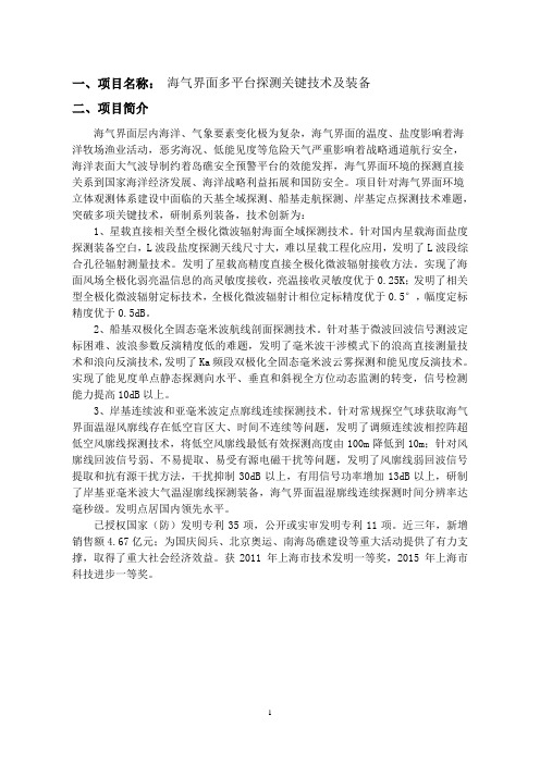
一、项目名称:海气界面多平台探测关键技术及装备二、项目简介海气界面层内海洋、气象要素变化极为复杂,海气界面的温度、盐度影响着海洋牧场渔业活动,恶劣海况、低能见度等危险天气严重影响着战略通道航行安全,海洋表面大气波导制约着岛礁安全预警平台的效能发挥,海气界面环境的探测直接关系到国家海洋经济发展、海洋战略利益拓展和国防安全。
项目针对海气界面环境立体观测体系建设中面临的天基全域探测、船基走航探测、岸基定点探测技术难题,突破多项关键技术,研制系列装备,技术创新为:1、星载直接相关型全极化微波辐射海面全域探测技术。
针对国内星载海面盐度探测装备空白,L波段盐度探测天线尺寸大,难以星载工程化应用,发明了L波段综合孔径辐射测量技术。
发明了星载高精度直接全极化微波辐射接收方法。
实现了海面风场全极化弱亮温信息的高灵敏度接收,亮温接收灵敏度优于0.25K;发明了相关型全极化微波辐射定标技术,全极化微波辐射计相位定标精度优于0.5°,幅度定标精度优于0.5dB。
2、船基双极化全固态毫米波航线剖面探测技术。
针对基于微波回波信号测波定标困难、波浪参数反演精度低的难题,发明了毫米波干涉模式下的浪高直接测量技术和浪向反演技术,发明了Ka频段双极化全固态毫米波云雾探测和能见度反演技术。
实现了能见度单点静态探测向水平、垂直和斜视全方位动态监测的转变,信号检测能力提高10dB以上。
3、岸基连续波和亚毫米波定点廓线连续探测技术。
针对常规探空气球获取海气界面温湿风廓线存在低空盲区大、时间不连续等问题,发明了调频连续波相控阵超低空风廓线探测技术,将低空风廓线最低有效探测高度由100m降低到10m;针对风廓线回波信号弱、不易提取、易受有源电磁干扰等问题,发明了风廓线弱回波信号提取和抗有源干扰方法,干扰抑制30dB以上,有用信号功率增加13dB以上,研制了岸基亚毫米波大气温湿廓线探测装备,海气界面温湿廓线连续探测时间分辨率达毫秒级。

HY-2A卫星校正微波辐射计数据用户手册国家卫星海洋应用中心2011年5月更改页目录1 数据产品介绍 (1)1.1 产品级别划分 (1)1.2 产品文件命名 (1)1.2.1 一级产品文件命名 (1)1.2.2 二级产品文件命名 (1)2 一级数据产品 (2)2.1 数据处理流程 (2)2.2 L 1A数据格式 (3)2.2.1 产品数据结构 (3)2.2.2 产品头文件 (4)2.2.3 产品科学数据 (6)2.2.4 科学数据各参数介绍 (9)2.3 L 1B数据格式 (14)2.3.1 产品数据结构 (14)2.3.2 产品头文件 (14)2.3.3 产品科学数据 (16)2.3.4 科学数据各参数介绍 (19)3 二级数据产品 (19)3.1 数据产品制作流程 (19)3.2 L 2A数据格式 (20)3.2.1 产品数据结构 (20)3.2.2 产品头文件 (20)3.2.3 产品科学数据 (23)3.2.4 科学数据各参数介绍 (25)3.3 L 2B数据格式 (25)3.3.1 产品数据结构 (25)3.3.2 产品头文件 (26)3.3.3 产品科学数据 (28)3.3.4 科学数据各参数介绍 (31)3.4 L 2C数据格式 (31)3.4.1 产品数据结构 (31)3.4.2 产品科学数据 (31)1数据产品介绍国家卫星海洋应用中心将载荷的HY-2卫星校正辐射计0级数据经过预处理、重采样和数据反演分别生成1级、2级产品。
1.1 产品级别划分一级产品1A:经过时间标识和地理定位后的数据。
包括扫描时间,每扫描点地理定位;存储观测、定标计数的数据;天线温度校正系数,轨道运行状态、平台姿态等辅助信息;记录质量信息等。
1B:经过分pass,亮温计算,以及带有定位信息及描述信息的数据。
二级产品2A:经过亮温重采样的数据,将1B中观测亮温平均成每秒一次。
2B:经过反演计算,将2A数据反演成海洋大气物理产品,并且包含2A的亮温产品。
多通道微波辐射计孙华磊;陈晓辉;郝立勇;程海平【摘要】本文介绍了一款被动式地基多通道微波辐射计,该辐射计利用被动的接收各个高度传来的温度辐射的微波信号来测量大气特性.地基微波辐射计可反演得到从地面至10 km 高度的温度、湿度和水汽廓线等大气信息,其观测是准连续的,观测时间步长小于3 min,可以弥补常规探空因观测间隔较长而获取大气信息的不足,有利于分析降水过程对流层快速变化的热力学信息和微尺度及中尺度现象的温度、湿度变化.【期刊名称】《电子世界》【年(卷),期】2017(000)021【总页数】1页(P99)【关键词】地基;多通道;波纹馈电【作者】孙华磊;陈晓辉;郝立勇;程海平【作者单位】安徽四创电子股份有限公司;安徽四创电子股份有限公司;安徽四创电子股份有限公司;安徽四创电子股份有限公司【正文语种】中文多通道微波辐射计是大气探测的重要手段之一,与地基探空雷达相比,成本低,无电磁污染,与探空气球相比,具有可以进行连续不间断观测的优点,能够实现其覆盖区域内气象要素的不间断观测,可应用于探测大气温度廓线、湿度廓线、水汽、云水含量、降水和大气成分等重要大气参数,在天气预报、大气科学研究领域具有巨大的市场需求.多通道微波辐射计(以下简称"辐射计")结合当前先进的电子技术,借鉴成熟的被动遥感探测技术,采用多通道反演大气温湿廓线,可以同时K波段和V波段两个频段的辐射信息.该辐射计开展数据的时空匹配、集成融合、质量互控技术研究,细化云属性分类及相态结构特征,提高反演温湿廓线及云中含水量特性分布的准确性,实现在气象研究、大气探测、航空保障及人工影响天气等领域的应用.辐射计采用波纹馈电喇叭天线.波纹馈电喇叭的反射损失小,结构紧凑,它可提供一个较宽的带宽、低的交叉极化电平和旋转对称的波束形式.天线覆盖的投影直径250mm,可在各个仰角上进行波束扫描.多通道辐射计有两个工作频率:K波段22~32 GHz (含7个直接滤波器通道,反演湿度廓线);V波段5~59 GHz (含7个直接滤波器通道,反演温度廓线).辐射计在设计是采用了成熟的可靠性设计、电磁兼容性设计、安全性设计和标准化设计,其平均无故障时间(MTBF)可以达到2500小时.该产品的接收器设计建立在不使用混频和本地振荡器进行下变频的直接检测技术的基础上,与采用传统的单检测器扫频微波辐射计相比,多通道并行滤波接收器组的特点是更精确、更稳定和更快速.大气辐射分频后分别进入K波段和V波段接收机,两个独立的接受模块(包括RF放大器、滤波器和检波二极管),允许同时测量大气温度和湿度,最大限度减小测量时间.当辐射计的天线主波束指向目标时,天线接收到目标辐射能量,引起天线视在温度的变化.反馈信号被天线接收后、经馈线进入接收分系统天线.接收的信号经过放大、滤波、检波和再放大后,以电压的形式给出.对微波辐射计的输出电压进行温度绝对定标,即建立输出电压与天线视在温度的关系之后,就可确定天线视在温度,也就可以确定所观测目标的亮温度.该温度值就包含了辐射体和传播介质的一些物理信息,通过数字信号处理系统输出数字信号就可以了解被探测目标的一些物理特性.信号处理输出数据至监控,监控将目标仰角、方位角的数字角度信号与繁衍出的亮温信号进行综合打包,送数据处理系统.监控同时控制伺服驱动完成天线扫描控制. 数据处理系统对数据进行实时处理,以各种扫描方式,实时显示数据信息.并可将数据存储下来.微波辐射计是基于大气微波遥感技术的气象观测设备,可实现对中尺度强天气系统大气层结的监测和预警、云物理特征的监测和人工影响天气科研及业务的应用、雾霾天气等边界层大气环境质量的监测.。
微波遥感基础微波遥感基础微波遥感基础 (1)⼀、微波遥感物理基础 (2)⼆、微波遥感技术的简介 (4)2.1 微波遥感 (4)2.2 微波遥感器 (5)2.2.1 雷达散射计 (5)2.2.2 微波辐射计 (5)2.2.3 雷达⾼度计 (6)2.3 微波遥感技术的特点 (7)2.4 微波遥感的优越性 (7)2.5 微波遥感的不⾜ (7)2.6 微波微波拥有强⼤⽣命⼒的根源 (7)2.7 我国微波遥感的差距 (8)三、雷达概念、分类 (8)3.1 成像雷达 (8)3.2 ⾮成像雷达 (8)3.3 真实孔径雷达 (9)3.4 合成孔径雷达 (9)3.5 极化雷达 (10)3.6 ⼲涉雷达 (11)3.7 激光雷达 (11)3.8 侧视雷达 (11)四、微波遥感图像 (11)4.1雷达图像 (11)4.1.1雷达图像 (11)4.1.2 雷达图像显⽰ (12)4.1.3 雷达图像分辨率 (12)4.1.4 雷达图像的处理 (12)4.2 侧视雷达图像 (13)4.3 雷达图像校准 (14)4.4 雷达图像定标 (14)4.5 雷达图像模拟 (14)五、微波遥感定标 (15)六、微波遥感概念、理论和技术的突破 (15)七、我国微波遥感的差距 (16)⼋、微波相关技术介绍 (17)8.1 偏振探测技术的特点 (17)8.2 微波散射特性 (18)九、微波遥感有待进⼀步研究的问题 (19)⼗、微波遥感的应⽤ (20)10.1 空间对地观测 (20)⼀、微波遥感物理基础电磁波具有波长(或频率)、传播⽅向、振幅和极化⾯(亦称偏振⾯)四个基本物理量。
极化⾯是是指电场振动⽅向所在的平⾯。
电磁波谱有时把波长在mm到km很宽的幅度内通称为⽆线电波区间,在这⼀区间按照波长由短到长⼜可以划分为亚毫⽶波、毫⽶波、厘⽶波、分⽶波、超短波、短波中波和长波。
其中的毫⽶波,厘⽶波和分⽶波三个区间称为微波波段,因此有时⼜更明确地吧这⼀区间分为微波波段和⽆线电波段。
微波遥感MicrowaveRemoteSensing一、课程基本情况课程类别:专业主干课课程学分:3学分课程总学时:48学时,其中讲课:32学时,实验(含上机):16学时课程性质:必修开课学期:第5学期先修课程:遥感原理1适用专业:遥感科学与技术教材:微波遥感原理,武汉大学出版社;舒宁,2003。
开课单位:地理与遥感学院遥感科学与技术系二、课程性质、敕学目标和任务本课程是遥感科学与技术专业方向专业主干课,是本专业必修课程之一。
通过对本课程的学习,使学生了解与掌握微波遥感的基本理论、原理与应用,了解微波遥感应用领域的最新发展。
进一步加强学生的遥感专业技能素养,扩宽遥感应用知识与技能。
微波遥感课程需要学生掌握微波电磁辐射基本原理、典型地物微波辐射特征、微波遥感平台及特点、微波遥感影像处理与应用、雷达干涉测量原理与应用,在此基础上了解微波遥感在不同领域内的应用。
同时通过对微波遥感的实习实践,培养学生在主被动微波遥感数据处理及解译的能力,加强学生在应用微波遥感方式解决遥感问题的应用技能,为学生微波遥感应用能力及进一步深造奠定基础。
三、教学内容和要求第1章微波遥感基础(6学时)1.1引言(1学时)(1)微波遥感概念;(2)微波遥感的优势与不足;(3)了解微波遥感的发展历史重点:微波遥感的优势与不足;1.2电磁波理论与微波(2学时)(1)掌握微波电磁波基本特征;(2)理解微波电磁辐射定律重点:微波电磁波特征与辐射定律;难点:微波电磁波辐射定律;1.3微波与物质的相互作用(2学时)(1)理解微波与大气的相互作用;(2)理解微波与地物的相关作用难点:微波与地物的相互作用;1.4微波遥感波段(1学时)(1)掌握常用微波遥感波段及各自特点。
重点:微波遥感常用波段;第2章微波遥感系统(8学时)2.1非成像微波传感器(1学时)(1)掌握微波散射计工作原理及应用;(2)掌握雷达高度计工作原理及应用;(3)了解无线电地下探测器工作原理及应用;重点:微波散射计工作原理及主要应用;2.2成像微波传感器(3学时)(1)掌握微波辐射计工作原理;(2)理解并掌握真实孔径侧视雷达工作原理;(4)掌握合成孔径侧视雷达工作原理;重点:成像雷达工作原理;难点:合成孔径雷达原理;2.3天线与雷达方程(2学时)(1)掌握天线的概念及主要参数;(2)掌握雷达方程与灰度方程的推导重点:天线的主要参数与雷达方程;难点:雷达方程的推导;2.4空间微波遥感系统(2学时)(1)了解主要的机载微波遥感系统;(2)了解主要的航天飞机微波遥感系统;(3)了解主要的卫星微波遥感系统;第3章微波图像的特点(8学时)3.1侧视雷达图像参数(1学时)(1)理解并掌握侧视雷达系统的主要工作参数;(2)理解雷达图像质量参数重点:侧视雷达系统的主要工作参数3.2雷达图像的几何特点(2学时)(1)理解并掌握雷达图像的斜距投影;(2)理解雷达图像的透视收缩和叠掩;(3)理解雷达阴影重点:雷达图像的几何变形特点;难点:雷达图像的透视收缩与叠掩;3.3雷达图像的信息特点(2学时)(1)了解地物目标的类型;(2)掌握影响雷达图像色调的主要因素;(3)了解并掌握雷达图像的主要虚假现象;重点:雷达图像色调的主要影响因素;3.4典型地物的散射特性(1学时)(1)掌握主要典型地物的散射特性;(2)掌握主要典型地物的微波热辐射特性难点:典型地物的散射特性;第四章微波遥感图像的校准、定标与模拟(2学时)4.1雷达回波的校准(0.5学时)(1)了解雷达系统内部校准原理与方法;(2)了解雷达系统内部校准原理与方法重点:雷达系统校准的主要方法;4.2雷达图像定标(0.5学时)(1)了解雷达图像定标的一般原理与方法4.3雷达图像模拟(0.5学时)(1)了解雷达图像模拟的一般原理与方法;4.4辐射计的校准与定标(0.5学时)(1)了解微波辐射计图像校准与定标的一般原理与方法;重点:雷达与微波辐射计图像的校准与定标;难点:雷达图像的校准与定标方法;第5章微波图像的几何校正(4学时)5.1雷达图像的几何变形分析(1学时)(1)了解造成雷达图像几何变形的主要原因;5.2侧视雷达图像的构像方程(1学时)(1)掌握基于等效中心投影的构像方程;(2)了解并掌握基于成像矢量关系和多普勒频率方程的构像方程;重点:侧视雷达图像的构像方程难点:基于成像矢量关系和多普勒频率方程的构像方程构建;5.3侧视雷达图像的几何校正方法(1学时)(1)掌握利用多项式与模拟图像的几何校正方法;(2)理解基于构像方程的几何校正方法重点:基于构像方程的几何校正方法第6章雷达干涉测量(4学时)6.1雷达干涉测量基本原理(2学时)(1)掌握干涉测量的基本概念;(2)理解并掌握雷达干涉测量原理;(3)掌握雷达干涉测量的主要工作方式难点:雷达干涉测量基本原理;6.2雷达干涉测量的主要应用(2学时)(1)理解雷达干涉测量的一般流程;(2)了解雷达干涉测量的主要应用;难点:相位解缠的概念及算法;第7章微波遥感应用(2学时)(3)了解微波辐射计的主要应用领域(4)了解雷达遥感技术在测绘、农业、城市、海洋、气象等领域的应用;(2)通过实例,了解微波遥感在资源环境中的应用方法,如土壤湿度遥感;四、课程考核(1)作业和报告:作业:5次左右;(2)考核方式:闭卷考试;(3)总评成绩计算方式:平时成绩、实验成绩、期中考试成绩和期末考试成绩等综合计算; (4)在多媒体教室开展教学活动,力求传统教学手段与现代技术的有机统一;五、参考书目1、雷达影像干涉测量原理,武汉大学出版社,舒宁,2003;2、雷达成像技术,电子工业出版社,保铮等,2005;3、微波遥感导论,科学出版社,lainH.Woodhouse,2014;4、遥感相关期刊。
Comparison of Calibration Techniques for Ground-Based C-Band RadiometersKai-Jen C.Tien,Student Member,IEEE,Roger D.De Roo,Member,IEEE,Jasmeet Judge,Senior Member,IEEE,and Hanh Pham,Student Member,IEEEAbstract—We quantify the performance of three commonly used techniques to calibrate ground-based microwave radiometers for soil moisture studies,external(EC),tipping-curve(TC),and internal(IC).We describe two ground-based C-band radiometer systems with similar design and the calibration experiments con-ducted in Florida and Alaska using these two systems.We compare the consistency of the calibration curves during the experiments among the three techniques and evaluate our calibration by com-paring the measured brightness temperatures(T B’s)to those estimated from a lake emission model(LEM).The mean absolute difference among the T B’s calibrated using the three techniques over the observed range of output voltages during the experiments was1.14K.Even though IC produced the most consistent calibra-tion curves,the differences among the three calibration techniques were not significant.The mean absolute errors(MAE)between the observed and LEM T B’s were about2–4K.As expected,the utility of TC at C-band was significantly reduced due to transparency of the atmosphere at these frequencies.Because IC was found to have a MAE of about2K that is suitable for soil moisture applications and was consistent during our experiments under different environmental conditions,it could augment less frequent calibrations obtained using the EC or TC techniques.Index Terms—Calibration,microwave radiometry,soil moisture.I.I NTRODUCTIONG ROUND-BASED microwave radiometers have been usedextensively to measure upwelling terrain emission in field experiments for hydrology,agriculture,and meteorology [1]–[7].The total-power radiometer is of the simplest design compared to other designs such as Dicke and noise injection[8] and[9].The stability and consistency of the relation between the output voltage and the antenna temperature,i.e.,system gain and offset,are critical for radiometer operations.The system gain is highly sensitive tofluctuations in the physical tempera-Manuscript received June5,2006;revised September29,2006.This work was supported in part by the National Aeronautics and Space Administration’s ESS Graduate Student Fellowship(ESSF03-0000-0044)and in part by the University of Florida,Institute of Food and Agricultural Sciences.K.-J.C.Tien and J.Judge are with the Center for Remote Sensing,De-partment of Agricultural and Biological Engineering,University of Florida, Gainesville FL32611USA(e-mail:ktien@ufl.edu;jasmeet@ufl.edu).R. D.De Roo is with the Department of Atmospheric,Oceanic,and Space Sciences,University of Michigan,Ann Arbor,MI48109USA(e-mail: deroo@).H.Pham is with the Department of Electrical Engineering and Com-puter Science,University of Michigan,Ann Arbor,MI48109USA(e-mail: hpham@).Color versions of one or more of thefigures in this paper are available online at .Digital Object Identifier10.1109/LGRS.2006.886420ture inside the radiometer requiring frequent calibration during radiometer operation for reliable and accurate observations. Many calibration techniques have been developed for mi-crowave radiometers for spaceborne and airborne[10]–[16] and ground-based radiometers[17]–[21].In general,calibration techniques include observations of radiometer output voltages for cold and hot targets with known brightness temperatures [8],[9].For radiometers operating at low frequencies away from the water vapor and oxygen absorption bands,such as C-band(6.7GHz),commonly used cold targets are liquid nitrogen or the sky.Hot targets include microwave absorbers or matched loads inside the radiometers.For a C-band ground-based microwave radiometer,the conceptually simplest cal-ibration technique using a microwave absorber at ambient temperature as a hot target is called“external calibration”(EC). Another widely used calibration technique that utilizes the sky measurements at different angles to calculate the optical depth of the atmosphere and the brightness temperatures of the sky is called“tipping curve calibration”(TC)[18],[19],[21].Either EC or TC can be used exclusively,or TC could be used to provide a better estimate of the sky measurement for EC.Both techniques are inconvenient to perform frequently for long-term soil moisture studies using ground-based C-band radiometers. Moreover,the utility of TC at C-band might be hampered by the high atmospheric transparency at low microwave frequencies [8].Another technique,“internal calibration”(IC),uses an internal matched load as the hot target.This technique has been used for spaceborne microwave radiometers,e.g.,SMMR [10],TMR[13],[14],and JMR[15],airborne radiometers [16],and ground-based radiometers[17].Unlike EC and TC, IC can be performed faster than gainfluctuation.Also,IC is neither sensitive to operator technique,to weathering of the delicate microwave absorber,nor does it require any additional hardware exclusively for the purpose of calibration.However, IC does not account for the losses in the antenna and trans-mission lines before the internal switch used to observe the matched load.In this letter,we quantify the performance of IC and validate it using EC and TC for long-term observations of soil moisture using two ground-based C-band radiometers.Our analysis is re-stricted to horizontal polarization(H-pol)because of its higher sensitivity to soil moisture than vertical polarization(V-pol)[8]. We describe two ground-based total-power radiometers with similar design:the University of Florida C-band Microwave Radiometer(UFCMR)and the C-band unit on the Truck Mounted Radiometer System3(TMRS-3C),as well as the calibration experiments conducted under significantly different1545-598X/$25.00©2007IEEETABLE IR ADIOMETER S PECIFICATIONS FOR UFCMR ANDTMRS-3Cenvironmental conditions in Florida and Alaska.We brieflysummarize three different calibration techniques and compare the consistency of the calibration among these techniques us-ing the two radiometers.We also discuss absolute accuracy of our brightness observations by comparing the observed brightness temperatures of a lake with those obtained using a lake emission model (LEM).II.C-B AND R ADIOMETERSThe UFCMR and TMRS-3C were developed by the Mi-crowave Geophysics Group at the University of Michigan (UM-MGG).Both are dual-polarized unbalanced total-power radiometers operating at the center frequency of 6.7GHz near the frequency of the Advanced Microwave Scanning Radiometer—EOS (AMSR-E)aboard the NASA Aqua Satel-lite.The UFCMR is mounted on a 10-m tower,whereas the TMRS-3C is mounted on a Norstar truck’s hydraulic arm,which can extend to 12m.TMRS-3consists of a suite of dual-polarized radiometers operating at 1.4,6.7,19,and 37GHz mounted on an elevation positioner that allows for approxi-mately 300◦rotation in the elevation axis.A major difference between the UFCMR and TMRS-3C designs is the use of two receivers for V-and H-pol in TMRS-3C,compared to only one receiver in the UFCMR that switches between the two polarizations.Table I lists the specifications of the C-band radiometers.III.F IELD E XPERIMENTSA.Microwave Water and Energy Balance Experiments (MicroWEXs)MicroWEXs were conducted by the Center for Remote Sensing,Department of Agricultural and Biological Engineer-ing,University of Florida,at the Plant Science Research and Education Unit (PSREU),IFAS,Citra,FL,during the growing seasons of cotton (MicroWEX-1[22]and -3[23])and corn (MicroWEX-2[24]).During the MicroWEXs,the UFCMR measured microwave brightness temperatures every 15min and was calibrated every two weeks.We conducted 10,4,and 11calibrations during the 140,80,and 190days of the MicroWEX-1,2,and 3,respectively.Each calibration included measurements of sky at zenith angles of 15◦,30◦,45◦,and 60◦,of a microwave absorber at ambient temperature,and of a matched load inside the radiometer.B.Tenth Radiobrightness and Energy Balance Experiment (REBEX-10)REBEX-10was conducted by the UM-MGG from May 6to July 1,2004,at a site about 1km north of Toolik Field Station on the North Slope of Alaska.In addition to conducting twice daily EC calibrations during REBEX-10,validation data were obtained by driving the Norstar truck to a beach on the northeast shore of Toolik Lake and extending the radiometer systems over the open water on June 21(DOY 173)and 22(DOY 174).The boom was extended to the west from the shore in the direction of the smallest solid angle of land presented at the opposite shore of the lake.The calibration targets included sky,absorber,and lake surface.The sky measurements were recorded at zenith angles of 0◦,10◦,23◦,30◦,32◦,40◦,and 55◦.The lake surface measurements were obtained at incidence angles of 23◦,30◦,32◦,40◦,and 55◦.The lake temperature was measured on DOY 173at 1502h (AKDT)to be 13.7◦C and on DOY 174at 0342h (AKDT)to be 10◦C.These are expected to be extreme lake temperatures during this period.IV .C ALIBRATION M ETHODOLOGYThe relationship between the output voltage (V out )and theantenna apparent temperature (TB)of a total-power radiome-ter with a square-law detector such as the UFCMR and the TMRS-3C can be expressed as follows:T B =S ·V out +I(1)where S and I are the slope and intercept of the calibration curve,respectively.A.External CalibrationThe calibration targets of EC included the microwave ab-sorber at ambient air temperature and the sky measurement at zenith angle of 15◦for UFCMR and 0◦for TMRS-3C.The S and I are S =(T B,sky −T abs )·η+(T ant ,sky −T ant ,abs )·(1−η)out ,sky −V out ,abs(2)I =T B.sky ·η+T ant ,sky ·(1−η)−S ·V out ,sky(3)where T abs is the physical temperature of the absorber (Kelvin),ηis the antenna efficiency,equal to 0.86±0.01,as estimated in the laboratory using one-port measurements with a network analyzer,T ant ,sky and T ant ,abs are the physical temperatures of antenna during the sky and absorber measurements,respec-tively (Kelvin),and V out ,sky and V out ,abs are the output voltages during the sky and absorber measurements,respectively (volts).T B,sky (Kelvin)given by [8]isT B,sky =T B,atm (θ)+T extra ·exp(−τ0·sec θ)(4)TIEN et al.:COMPARISON OF CALIBRATION TECHNIQUES FOR GROUND-BASED C-BAND RADIOMETERS85 andT B,atm(θ)=secθ∞κa(z )·T(z )exp(−τ(0,z )·secθ)dz(5)where T extra is the extraterrestrial brightness temperature (Kelvin),which is∼2.7K,τ0is the total zenith opacity(Np),θis the zenith angle,κa is the atmospheric absorption coef-ficient(Np·m−1),T is the temperature profile(Kelvin),andτ(0,z )is the optical thickness of the atmosphere between the surface and height z (Np).Given the atmospheric temper-ature,pressure,and water vapor density,the sky brightness temperatures can be calculated based on the1962U.S.Standard Atmosphere[8].At C-band,the sensitivity of sky brightness to changes in atmospheric conditions can be ignored due to the high atmospheric transparency[8].The sources of error using EC include the measurement er-rors due to the antenna sidelobes,εsl,the insertion loss variabil-ity of the radiometer switches,εsw,and the uncertainty in the physical temperature measurements of the absorberεat.While errors due to measurement of antenna efficiency contribute to errors in antenna noise temperatures,these errors are removed in the correction to scene brightness temperatures because the calibration targets are all external to the antenna.The effect of these errors using UFCMR and TMRS-3C will be discussed in Section V.B.TC CalibrationT B,sky can be obtained by TC assuming a horizontally strat-ified atmosphere[19]and[25]asT B,sky=T extra·exp[−A(θ)·τ]+T atm·(1−exp[−A(θ)·τ])(6) where A is the airmass at zenith angleθ,τis the atmospheric opacity(Np),and T atm is the mean atmospheric temperature (Kelvin).For UFCMR and TMRS-3C,the antenna temperature is linearly related to the output voltage such thatV out,sky−V out,abs V out,abs−V ofst =T A,sky−T A,absT A,abs−T rec(7)where V ofst is the system offset voltage when the system input noise temperature is0K(T sys=T A+T rec),T A,sky and T A,abs are the apparent antenna temperatures for the sky and absorber measurements,respectively(Kelvin),and T rec is the receiver noise temperature(Kelvin).The equations for S and I are the same as(2)and(3),with T B,sky estimated by the radia-tive transfer equation using the least-squares technique from 0◦to45◦.The atmospheric temperature was approximated by the air temperature at the Earth’s surface[19].The sources of error using TC includeεsl,εsw,andεat, similar to those in EC.Errors in antenna noise temperatures due to uncertainty in the antenna efficiency are removed in the correction to scene brightness temperatures.C.Internal CalibrationIC uses an internal matched load or afixed-temperature source,such as a noise diode,inside the radiometer as the hot target.The cold target is the sky measurement at15◦for UFCMR and at0◦for TMRS-3C.The S and I using IC are S=T B,sky·η+T ant,sky·(1−η)−T calV out,sky−V out,cal(8)I=T cal−S·V out,cal(9) where T cal is the physical temperature of the matched load (Kelvin),ηis the antenna efficiency,V out,cal is the output voltage when switched to the matched load at T cal(volts),and T B,sky is estimated,similar to EC[8].The sources of error using IC include theεsl andεsw,similar to those in EC,the error due to the uncertainty in the antenna efficiency estimationεae and the uncertainty in the physical temperature measurements of the internal loadεlt.D.LEMFor an open calm water surface,the brightness temperatures observed by a microwave radiometer can be modeled asT B,p=Γp·T B,sky+(1−Γp)·T water(10) whereΓp is the reflectivity at polarization p,and T water is the physical temperature of water(Kelvin).T B,sky is∼5K for C-band.The reflectivity of the specular water surface is deter-mined by the incidence angle[26]and the dielectric constant of the water.The empirical models used for the dielectric constant of pure water can be found in[27]and[28].V.R ESULTS AND D ISCUSSIONThe calibration data from MicroWEXs and REBEX-10pro-vided a unique opportunity to compare the performance of two C-band radiometers with similar design in different environ-mental conditions.During each experiment,the radiometers were maintained at constant temperatures with0.1K standard deviation at the RF circuitry.Table II shows the means and the standard deviations of the calibration curves at H-pol during MicroWEXs and REBEX-10.These included25data points during MicroWEXs,as well as80points for EC and IC,and two points for TC during REBEX-10.IC produced the most consistent calibration curves in terms of the lowest standard deviations of the slopes,although the differences among the calibration techniques were not significant.Fig.1(a)–(d)shows the gainfluctuations of the calibration curves for MicroWEXs and REBEX-10.The mean absolute dif-ference(MAD)between the slopes of EC and IC was2.8K/V during MicroWEXs.The difference between the slopes of TC and EC was4.4K/V,and the difference between the slopes of TC and IC was3.6K/V during MicroWEXs.The MADs for REBEX-10were not calculated because there were only two TC measurements.During MicroWEXs,the EC and IC calibration curves were closer to each other,while TC produced slightly dissimilar results from EC and IC.This was primarily86IEEE GEOSCIENCE AND REMOTE SENSING LETTERS,VOL.4,NO.1,JANUARY 2007TABLE IIM EAN AND S TANDARD D EVIATION OF THE S LOPES (S )AND I NTERCEPTS (I )FOR THE H-P OL C ALIBRATION C URVE D URING M ICRO WEX S (MWS)AND REBEX-10(RB)Fig.1.Slopes for the calibration curve at H-pol during (a)MicroWEX-1,(b)2,(c)3,and (d)REBEX-10.RMSE of EC =1.20,TC =1.84,and IC =1.10K/V.For clarity of the figures,only Fig.1(a)shows the error bars.because at C-band,TC is based on multiple measurements with small differences in brightness temperatures (T B ’s)of the sky,compared to measurements at higher frequencies at which the differences are larger.Due to the high atmospheric transparency,the utility of TC at C-band was reduced.Applying the calibration curves over the output voltages for the terrains observed during MicroWEXs and REBEX-10,the MAD of the calibrated T B ’s using the three calibration techniques was 1.14K.Table III gives the root-mean-square errors (RMSEs)estimates in the accuracy of observed T B ’s using UFCMR and TMRS-3C due to εae ,εsl ,εsw ,εat ,and εlt ,as mentioned in Section IV.The RMSE of EC,TC,and IC are 1.20,1.84,and 1.10K/V ,respectively.To assess the accuracy of the calibration,we observed T B ’s of a calm lake at different incidence angles between 20◦and 55◦during REBEX-10.The RMSEs due to antenna sidelobes dur-ing the lake observations were 0.28,0.26,0.25,0.25,and 0.24K at incidence angles of 23◦,30◦,32◦,40◦,and 55◦,respectively.These RMSEs are included in the error bars shown in Fig.2(a)and (b).Observed T B ’s were compared with those of a smooth water surface simulated by LEM (Fig.2).We usedTABLE IIIRMSE E STIMATION FOR THE O PERATION AND C ALIBRATION OF UFCMR ANDTMRS-3Cparison of differences between the REBEX-10observed and LEM simulated brightness temperatures (∆T B )(a)at H-pol on DOY 173and (b)at H-pol on DOY 174.The total RMSE between observed and simulated values are 1.46,2.20,and 1.39for EC,TC,and IC,respectively.two dielectric models for pure water,[27],[28]and found that the MADs between the simulated LEM T B ’s were insignificant at ∼0.0095K.The uncertainty in the measurements of physical temperature of water was ±3.0K resulting in an RMSE of 0.8K at H-pol in the simulated T B ’s.The mean absolute errors (MAE)between the observed and modeled T B ’s at H-pol were 2.50±1.46,3.90±2.02,and 2.40±1.39K for EC,TC,and IC,respectively.For soil moisture applications,an accuracy of about 2K at C-band is adequate [29].VI.C ONCLUSIONThe calibration experiments during the MicroWEXs and REBEX-10were designed to assess the calibration consistency of two C-band radiometers with similar design.We compare the three most widely used techniques EC,TC,and IC to understand their performance for long-term soil moisture stud-ies using ground-based C-band radiometers.Even though IC produced the most consistent calibration curves,the differ-ences among the three calibration techniques were not signif-icant.Applying the calibration curves over the range of output voltages observed during the MicroWEXs and REBEX-10,TIEN et al.:COMPARISON OF CALIBRATION TECHNIQUES FOR GROUND-BASED C-BAND RADIOMETERS87the MAD of the T B’s calibrated among the three calibrationtechniques was1.14K.The absolute accuracy of calibrationtechniques was investigated by comparing the observed andmodeled T B’s of a calm lake.The MAE between the observedand modeled T B’s were2.50±1.46,3.90±2.02,and2.40±1.39K at H-pol for EC,TC,and IC,respectively.Due to the high atmospheric transparency,the utility of TC at C-band isgreatly reduced.Because IC was found to have a MAE of∼2K,suitable for soil moisture applications,and was consistent dur-ing our experiments under significantly different environmentalconditions,it can be used to augment less frequent calibrationsobtained by the EC or TC techniques.A CKNOWLEDGMENTThe authors would like to thank the anonymous reviewersfor their constructive comments and suggestions that improvedthis paper.The authors would also like to thank T.Lin,J.Casanova,M.-Y.Jang,ler,and nni for theirsupport during the MicroWEXs,the PSREU Research Coor-dinator J.Boyer and his team for providing excellent manage-ment of the studyfields,and M.Dukes(University of Florida)for providing the measurements of air pressure and temperatureused for calibrating the UFCMR.R EFERENCES[1]T.J.Jackson and P.E.O’Neill,“Attenuation of soil microwave emissionby corn and soybean at1.4and5GHz,”IEEE Trans.Geosci.Remote Sens.,vol.28,no.5,pp.978–980,Sep.1990.[2]T.J.Jackson,P.E.O’Neill,and C.T.Swift,“Passive microwave observa-tion of diurnal surface soil moisture,”IEEE Trans.Geosci.Remote Sens., vol.35,no.5,pp.1210–1222,Sep.1997.[3]J.Judge,J.F.Galantowicz,and A.W.England,“A comparison of ground-based and satellite-borne microwave radiometric observations in the Great Plains,”IEEE Trans.Geosci.Remote Sens.,vol.39,no.8,pp.1686–1696, Aug.2001.[4]J.Shi,K.S.Chen,Q.Li,T.J.Jackson,P.E.O’Neill,and L.Tsang,“A pa-rameterized surface reflectivity model and estimation of bare-surface soil moisture with L-band radiometer,”IEEE Trans.Geosci.Remote Sens., vol.40,no.12,pp.2674–2686,Dec.2002.[5]F.Lemaitre,J.C.Poussiere,Y.H.Kerr,M.Dejus,R.Durbe,P.Rosnay,and J.C.Calvet,“Design and test of the ground-based L-band radiometer for estimating water in soil(LEWIS),”IEEE Trans.Geosci.Remote Sens., vol.42,no.8,pp.1666–1676,Aug.2004.[6]K.Schneeberger, C.Stamm, C.Matzler,and H.Fluhler,“Ground-based dual-frequency radiometry of bare soil at high temporal resolu-tion,”IEEE Trans.Geosci.Remote Sens.,vol.42,no.3,pp.588–595, Mar.2004.[7]A.Memmo,E.Fionda,T.Paolucci,D.Cimini,R.Ferretti,S.Bonafoni,and P.Ciotti,“Comparison of MM5integrated water vapor with mi-crowave radiometer,GPS,and radiosonde measurements,”IEEE Trans.Geosci.Remote Sens.,vol.43,no.5,pp.1050–1058,May2005.[8]F.T.Ulaby,R.K.Moore,and A.K.Fung,Microwave RemoteSensing—Active and Passive,vol.I.Norwood,MA:Artech House, 1981,pp.369–396.[9]N.Skou,Microwave Radiometer Systems:Design and Analysis.Norwood,MA:Artech House,1989,pp.13–19.[10]E.Njoku,J.M.Stacey,and F.T.Barath,“The Seasat Scanning MicrowaveRadiometer(SMMR):Instrument description and performance,”IEEE J.Ocean.Eng.,vol.OE-5,no.2,pp.100–115,Apr.1980.[11]C.S.Ruf,“Detection of calibration drifts in spaceborne microwave ra-diometers using a vicarious cold reference,”IEEE Trans.Geosci.Remote Sens.,vol.38,no.1,pp.44–52,Jan.2000.[12]C.S.Ruf and J.Li,“A correlated noise calibration standard for interfer-ometric,polarimetric,and autocorrelation microwave radiometers,”IEEE Trans.Geosci.Remote Sens.,vol.41,no.10,pp.2187–2196,Oct.2003.[13]C.S.Ruf,S.J.Keihm,and M.A.Janssen,“TOPEX/Poseidon MicrowaveRadiometer(TMR).I.Instrument description and antenna temper-ature calibration,”IEEE Trans.Geosci.Remote Sens.,vol.33,no.1, pp.125–137,Jan.1995.[14]C.S.Ruf,S.J.Keihm, B.Subramanya,and M. A.Janssen,“TOPEX/POSEIDON Microwave Radiometer performance and in-flight calibration,”J.Geophys.Res.,vol.99,no.C12,pp.24915–24926,1994.[15]P.Bonnefond,B.Haines,G.Born,P.Exertier,S.Gill,G.Jan,E.Jeansou,D.Kubitscheck,urain,Y.Menard,and A.Orsoni,“Calibrating theJason-1measurement system:Initial results from the Corsica and Harvest verification experiments,”Adv.Space Res.,vol.32,no.11,pp.2135–2140, 2003.[16]I.Corbella,A.J.Gasiewski,M.Klein,V.Leuski,A.J.Francavilla,andJ.R.Piepmeier,“On-board calibration of dual-channel radiometers using internal and external references,”IEEE Trans.Microw.Theory Tech., vol.50,no.7,pp.1816–1820,Jul.2002.[17]H.Pham,E.J.Kim,and A.W.England,“An analytical calibration ap-proach for microwave polarimetric radiometers,”IEEE Trans.Geosci.Remote Sens.,vol.43,no.11,pp.2443–2451,Nov.2005.[18]B.Deuber,N.Kampfer,and D.G.Feist,“A new22-GHz radiometerfor middle atmospheric water vapor profile measurements,”IEEE Trans.Geosci.Remote Sens.,vol.42,no.5,pp.974–984,May2004.[19]Y.Han and E.R.Westwater,“Analysis and improvement of tipping cal-ibration for ground-based microwave radiometer,”IEEE Trans.Geosci.Remote Sens.,vol.38,no.3,pp.1260–1276,May2000.[20]K.Al-Ansari,P.Garcia,J.M.Riera,A.Benarroch,D.Fernandez,andL.Fernandez,“Calibration procedure of a microwave total-power radiometer,”IEEE Microw.Wireless Compon.Lett.,vol.12,no.3, pp.93–95,Mar.2002.[21]D.Cimini,E.R.Westwater,Y.Han,and S.J.Keihm,“Accuracy ofground-based microwave radiometer and balloon-borne measurements during the WVIOP2000field experiment,”IEEE Trans.Geosci.Remote Sens.,vol.41,no.11,pp.2605–2615,Nov.2003.[22]K.C.Tien,J.Judge,ler,and nni,Field Data Reportfor the First Microwave Water and Energy Balance Experiment (MicroWEX-1)July17–Decemb er16,2003,Gainesville,FL:Center for Remote Sensing,Univ.Florida,2005.[Online].Available:http://edis.ifas.ufl.edu/AE288[23]T.Lin,J.Judge,K.C.Tien,J.J.Casanova,M.Jang,nni,L.W.Miller,and F.Yan,Field Observations During the Third Microwave Water and Energy Balance Experiment(MicroWEX-3)June16–Decemb er21, 2004,Gainesvile,FL:Center for Remote Sensing,Univ.Florida,2005.[Online].Available:http://edis.ifas.ufl.edu/AE361[24]J.Judge,J.J.Casanova,T.Lin,K.C.Tien,M.Jang,nni,andler,Field Observations During the Second Microwave Wa-ter and Energy Balance Experiment(MicroWEX-2)March17–June3, 2004,Gainesville,FL:Center for Remote Sensing,Univ.Florida,2005.[Online].Available:http://edis.ifas.ufl.edu/AE360[25]M.A.Janssen,Atmospheric Remote Sensing by Microwave Radiometry.New York:Wiley,1993,pp.259–334.[26]L.A.Rose,W.E.Asher,S.C.Reising,P.W.Gasier,K.M.St.Germain,D.J.Dowgiallo,K.Horgan,G.Farquharson,andE.J.Knapp,“Radio-metric measurements of the microwave emissivity of foam,”IEEE Trans.Geosci.Remote Sens.,vol.40,no.12,pp.2619–2625,Dec.2002. [27]L.A.Klein and C.T.Swift,“An improved model for the dielectricconstant of sea water at microwave frequencies,”IEEE Trans.Antennas Propag.,vol.AP-25,no.1,pp.104–111,Jan.1977.[28]T.Meissner and F.J.Wentz,“The complex dielectric constant of pure andsea water from microwave satellite observations,”IEEE Trans.Geosci.Remote Sens.,vol.42,no.9,pp.1836–1849,Sep.2004.[29]J. C.Calvet, A.Chanzy,and J.P.Wigneron,“Surface temperatureand soil moisture retrieval in the Sahel from airborne multifrequency microwave radiometry,”IEEE Trans.Geosci.Remote Sens.,vol.34,no.2, pp.588–600,Mar.1996.。