模式识别实验报告
- 格式:docx
- 大小:155.44 KB
- 文档页数:15


基于K-L 变换的iris 数据分类一、实验原理K-L 变换是一种基于目标统计特性的最佳正交变换。
它具有一些优良的性质:即变换后产生的新的分量正交或者不相关;以部分新的分量表示原矢量均方误差最小;变换后的矢量更趋确定,能量更集中。
这一方法的目的是寻找任意统计分布的数据集合之主要分量的子集。
设n 维矢量12,,,Tn x x x ⎡⎤⎣⎦=x ,其均值矢量E ⎡⎤⎣⎦=μx ,协方差阵()T x E ⎡⎤⎣⎦=--C x u)(x u ,此协方差阵为对称正定阵,则经过正交分解克表示为x =T C U ΛU ,其中12,,,[]n diag λλλ=Λ,12,,,n u u u ⎡⎤⎣⎦=U 为对应特征值的特征向量组成的变换阵,且满足1T -=U U 。
变换阵T U 为旋转矩阵,再此变换阵下x 变换为()T -=x u y U ,在新的正交基空间中,相应的协方差阵12[,,,]x n diag λλλ==x UC U C 。
通过略去对应于若干较小特征值的特征向量来给y 降维然后进行处理。
通常情况下特征值幅度差别很大,忽略一些较小的值并不会引起大的误差。
对经过K-L 变换后的特征向量按最小错误率bayes 决策和BP 神经网络方法进行分类。
二、实验步骤(1)计算样本向量的均值E ⎡⎤⎣⎦=μx 和协方差阵()T x E ⎡⎤⎣⎦=--C x u)(x u 5.8433 3.0573 3.7580 1.1993⎡⎤⎢⎥⎢⎥⎢⎥⎢⎥⎢⎥⎣⎦=μ,0.68570.0424 1.27430.51630.04240.189980.32970.12161.27430.3297 3.1163 1.29560.51630.1216 1.29560.5810x ⎡⎤⎢⎥⎢⎥⎢⎥⎢⎥⎢⎥⎣⎦----=--C (2)计算协方差阵x C 的特征值和特征向量,则4.2282 , 0.24267 , 0.07821 , 0.023835[]diag =Λ-0.3614 -0.6566 0.5820 0.3155 0.0845 -0.7302 -0.5979 -0.3197 -0.8567 0.1734 -0.0762 -0.4798 -0.3583 0.0755 -0.5458 0.7537⎡⎤⎢⎥⎢⎥⎢⎥⎢⎥⎢⎥⎣⎦=U 从上面的计算可以看到协方差阵特征值0.023835和0.07821相对于0.24267和4.2282很小,并经计算个特征值对误差影响所占比重分别为92.462%、5.3066%、1.7103%和0.52122%,因此可以去掉k=1~2个最小的特征值,得到新的变换阵12,,,new n k u u u -⎡⎤⎣⎦=U 。

模式识别理论与方法
课程作业实验报告
实验名称:Generating Pattern Classes
实验编号:Proj02-01
规定提交日期:2012年3月30日
实际提交日期:2012年3月24日
摘要:
在熟悉贝叶斯分类器基本原理基础上,通过对比分类特征向量维数差异而导致分类正确率发生的变化,验证了“增加特征向量维数,可以改善分类结果”。
对于类数的先验概率已知、且无须考虑代价函数的情况,贝叶斯分类器相当简单:“跟谁亲近些,就归属哪一类”。
技术论述:
1,贝叶斯分类器基本原理:多数占优,错误率最小,风险最低
在两类中,当先验概率相等时,贝叶斯分类器可以简化如下:
2,增加有效分类特征分量,可以有助于改善分类效果
实验结果讨论:
从实验的过程和结果来看,进一步熟悉了贝叶斯分类器的原理和使用,基本达到了预期目的。
实验结果:
图1 原始数据
图2 按第1 个特征分量分类结果
图3 按第2 个特征分量分类结果
图4 综合两个特征分量分类结果附录:(程序清单,参见压缩包)
%在Matlab 版本2009a 下运行通过。

《模式识别》实验报告三、线性分类器实验1.(a)产生两个都具有200 个二维向量的数据集X1 和X1 ’。
向量的前半部分来自m1=[-5;0]的正态分布,并且S1=I 。
向量的后半部分来自m2=[5;0]的正态分布,并且S1=I。
其中I是一个2×2 的单位矩阵。
(b)在上面产生的数据集上运用Fisher 线性判别、感知器算法和最小平方误差判别算法,需要初始化参数的方法使用不同的初始值。
(c)测试每一种方法在X1 和X1 ’ 上的性能(错误率)。
(d)画出数据集X1 和X1 ’,已经每种方法得到对应参数向量W 的分界线。
Fisher线性判别图1 红色为第一类,绿色为第二类,直线为对应参数向量W的分界线,参数向量w = [-9.9406, 0.9030]’错误率error=0,感知器算法:图2 红色为第一类,绿色为第二类,直线为对应参数向量W的分界线,参数的初始值为[0.1;0.1];迭代次数iter=2参数向量w = [-4.8925, 0.0920]’错误率error=0图3 红色为第一类,绿色为第二类,直线为对应参数向量W的分界线,参数的初始值为[1; 1];迭代次数iter=2参数向量w = [-3.9925, 0.9920]’错误率error=0图4 红色为第一类,绿色为第二类,直线为对应参数向量W的分界线,参数的初始值为[10; 10];迭代次数iter=122参数向量w = [-5.6569, 7.8096]’错误率error=0图5 红色为第一类,绿色为第二类,直线为对应参数向量W的分界线,参数的初始值为[50; 50];迭代次数iter=600参数向量w = [-27.0945, 37.4194]’错误率error=0图6 红色为第一类,绿色为第二类,直线为对应参数向量W的分界线,参数的初始值为[50; 100];迭代次数iter=1190参数向量w = [-54.0048, 74.5875]’错误率error=0最小平方误差判别算法:图7 红色为第一类,绿色为第二类,直线为对应参数向量W的分界线,参数的初始值为[0.1; 0.1];参数向量w = [-0.1908, -0.0001]’错误率error=0图8 红色为第一类,绿色为第二类,直线为对应参数向量W的分界线,参数的初始值为[0.5; 0.5];参数向量w = [-0.1924, 0.1492]’错误率error=0图9 红色为第一类,绿色为第二类,直线为对应参数向量W的分界线,参数的初始值为[1; 0.5];参数向量w = [-0.1914, 0.0564]’错误率error=0图10 红色为第一类,绿色为第二类,直线为对应参数向量W的分界线,参数的初始值为[1; 1];参数向量w = [-0.1943, 0.3359]’错误率error= 0.00502.重复1.中的实验内容,数据集为X2 和X2 ’。
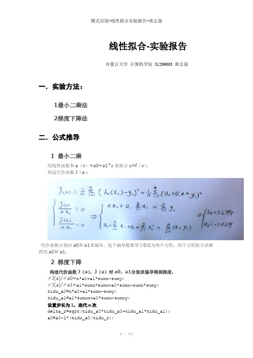
线性拟合-实验报告内蒙古大学计算机学院31209003 黄志强一.实验方法:1最小二乘法2梯度下降法二.公式推导1 最小二乘用线性函数h a(x)=a0+a1*x来拟合y=f(x);构造代价函数J(a):代价函数分别对a0和a1求偏导,连个偏导数都等于0成为两个方程,两个方程联合求解得到a0和a1;2 梯度下降构造代价函数J(a),J(a)对a0,a1分别求偏导得到梯度,〆J(a)/〆a0=n*a0+a1*sumx-sumy;〆J(a)/〆a1=a1*sumx*sumx+a0*sumx-sumx*sumy;tidu_a0=n*a0+a1*sumx-sumy;tidu_a1=a1*sumxx+a0*sumx-sumxy;设置步长为l,迭代m次delta_r=sqrt(tidu_a0*tidu_a0+tidu_a1*tidu_a1);a0=a0-l*(tidu_a0/tidu_r);a1=a1-l*(tidu_a1/tidu_r);每次迭代显示得到的直线和mse,并修订学习率%显示直线x2=[-0.1,1.1];y2=x2.*a1+a0;plot(x2,y2,'color',[1-i/m,1-i/m,1-i/m]);%显示错误error=0;for j=1:nerror=error+(y(j)-(a1*x(j)+a0))*(y(j)-(a1*x(j)+a0));endmse=error/n;l=mse;mse三.matlab代码1 最小二乘法代码:%in是一个100行2列的矩阵,两列分别为x和y。
用一条直线y=x*a+b拟合x和y 的关系;%用最小二乘法计算a和b。
x=in(1:100,1);y=in(1:100,2);sumx=0;sumy=0;sumxx=0;sumyy=0;sumxy=0;for i=1:1:100sumx=sumx+x(i);sumy=sumy+y(i);sumxx=sumxx+x(i)*x(i);sumyy=sumyy+y(i)*y(i);sumxy=sumxy+x(i)*y(i);endplot(in(:,1),in(:,2),'r.'); %用红色的点画出100个样本点hold on; %保留当前绘图,不被下次绘图遮盖n=100;[b,a]=solve('n*a0+a1*sumx=sumy','a0*sumx+a1*sumxx=sumxy','a 0','a1');%解二元一次方程组,未知数为a0,a1,结果返回给b和a。

《模式识别》大作业人脸识别方法二---- 基于PCA 和FLD 的人脸识别的几何分类器(修改稿)一、 理论知识1、fisher 概念引出在应用统计方法解决模式识别问题时,为了解决“维数灾难”的问题,压缩特征空间的维数非常必要。
fisher 方法实际上涉及到维数压缩的问题。
fisher 分类器是一种几何分类器, 包括线性分类器和非线性分类器。
线性分类器有:感知器算法、增量校正算法、LMSE 分类算法、Fisher 分类。
若把多维特征空间的点投影到一条直线上,就能把特征空间压缩成一维。
那么关键就是找到这条直线的方向,找得好,分得好,找不好,就混在一起。
因此fisher 方法目标就是找到这个最好的直线方向以及如何实现向最好方向投影的变换。
这个投影变换恰是我们所寻求的解向量*W ,这是fisher 算法的基本问题。
样品训练集以及待测样品的特征数目为n 。
为了找到最佳投影方向,需要计算出各类均值、样品类内离散度矩阵i S 和总类间离散度矩阵w S 、样品类间离散度矩阵b S ,根据Fisher 准则,找到最佳投影准则,将训练集内所有样品进行投影,投影到一维Y 空间,由于Y 空间是一维的,则需要求出Y 空间的划分边界点,找到边界点后,就可以对待测样品进行进行一维Y 空间的投影,判断它的投影点与分界点的关系,将其归类。
Fisher 法的核心为二字:投影。
二、 实现方法1、 一维实现方法(1) 计算给类样品均值向量i m ,i m 是各个类的均值,i N 是i ω类的样品个数。
11,2,...,ii X im X i nN ω∈==∑(2) 计算样品类内离散度矩阵iS 和总类间离散度矩阵wS1()()1,2,...,i Ti i i X w ii S X m X m i nS Sω∈==--==∑∑(3) 计算样品类间离散度矩阵b S1212()()Tb S m m m m =--(4) 求向量*W我们希望投影后,在一维Y 空间各类样品尽可能地分开,也就是说我们希望两类样品均值之差(12m m -)越大越好,同时希望各类样品内部尽量密集,即希望类内离散度越小越好,因此,我们可以定义Fisher 准则函数:()Tb F Tw W S W J W W S W=使得()F J W 取得最大值的*W 为 *112()w WS m m -=-(5) 将训练集内所有样品进行投影*()Ty W X =(6) 计算在投影空间上的分割阈值0y在一维Y 空间,各类样品均值i m为 11,2,...,ii y imy i n N ω∈==∑样品类内离散度矩阵2i s和总类间离散度矩阵w s 22()ii iy sy mω∈=-∑21w ii ss==∑【注】【阈值0y 的选取可以由不同的方案: 较常见的一种是1122012N m N m y N N +=+另一种是121201ln(()/())22m m P P y N N ωω+=++- 】(7) 对于给定的X ,计算出它在*W 上的投影y (8) 根据决策规则分类0102y y X y y X ωω>⇒∈⎧⎨<⇒∈⎩2、程序中算法的应用Fisher 线性判别方法(FLD )是在Fisher 鉴别准则函数取极值的情况下,求得一个最佳判别方向,然后从高位特征向量投影到该最佳鉴别方向,构成一个一维的判别特征空间将Fisher 线性判别推广到C-1个判决函数下,即从N 维空间向C-1维空间作相应的投影。
2015年12月实验一 Bayes 分类器的设计一、 实验目的:1. 对模式识别有一个初步的理解,能够根据自己的设计对贝叶斯决策理论算法有一个深刻地认识;2. 理解二类分类器的设计原理。
二、 实验条件:1. PC 微机一台和MATLAB 软件。
三、 实验原理:最小风险贝叶斯决策可按下列步骤进行:1. 在已知)(i P ω,)|(i X P ω,c i ,,1 =及给出待识别的X 的情况下,根据贝叶斯公式计算出后验概率:∑==c j jj i i i P X P P X P X P 1)()|()()|()|(ωωωωω c j ,,1 =2. 利用计算出的后验概率及决策表,按下式计算出采取i α决策的条件风险: ∑==c j j j i i X P X R 1)|(),()|(ωωαλα a i ,,1 =3. 对2中得到的a 个条件风险值)|(X R i α(a i ,,1 =)进行比较,找出使条件风险最小的决策k α,即:)|(min )|(,,1X R X R k c i k αα ==, 则k α就是最小风险贝叶斯决策。
四、 实验内容:假定某个局部区域细胞识别中正常(1ω)和非正常(2ω)两类先验概率分别为: 正常状态:)(1ωP =0.9;异常状态:)(2ωP =0.1。
现有一系列待观察的细胞,其观察值为x :-3.9847 -3.5549 -1.2401 -0.9780 -0.7932 -2.8531-2.7605 -3.7287 -3.5414 -2.2692 -3.4549 -3.0752-3.9934 2.8792 -0.9780 0.7932 1.1882 3.0682-1.5799 -1.4885 -0.7431 -0.4221 -1.1186 4.2532)|(1ωx P )|(2ωx P 类条件概率分布正态分布分别为(-2,0.25)(2,4)。
决策表为011=λ(11λ表示),(j i ωαλ的简写),12λ=6, 21λ=1,22λ=0。
《模式识别》实验报告班级:电子信息科学与技术13级02 班姓名:学号:指导老师:成绩:通信与信息工程学院二〇一六年实验一 最大最小距离算法一、实验内容1. 熟悉最大最小距离算法,并能够用程序写出。
2. 利用最大最小距离算法寻找到聚类中心,并将模式样本划分到各聚类中心对应的类别中.二、实验原理N 个待分类的模式样本{}N X X X , 21,,分别分类到聚类中心{}N Z Z Z , 21,对应的类别之中.最大最小距离算法描述:(1)任选一个模式样本作为第一聚类中心1Z 。
(2)选择离1Z 距离最远的模式样本作为第二聚类中心2Z 。
(3)逐个计算每个模式样本与已确定的所有聚类中心之间的距离,并选出其中的最小距离.(4)在所有最小距离中选出一个最大的距离,如果该最大值达到了21Z Z -的一定分数比值以上,则将产生最大距离的那个模式样本定义为新增的聚类中心,并返回上一步.否则,聚类中心的计算步骤结束。
这里的21Z Z -的一定分数比值就是阈值T ,即有:1021<<-=θθZ Z T(5)重复步骤(3)和步骤(4),直到没有新的聚类中心出现为止。
在这个过程中,当有k 个聚类中心{}N Z Z Z , 21,时,分别计算每个模式样本与所有聚类中心距离中的最小距离值,寻找到N 个最小距离中的最大距离并进行判别,结果大于阈值T 是,1+k Z 存在,并取为产生最大值的相应模式向量;否则,停止寻找聚类中心。
(6)寻找聚类中心的运算结束后,将模式样本{}N i X i ,2,1, =按最近距离划分到相应的聚类中心所代表的类别之中。
三、实验结果及分析该实验的问题是书上课后习题2。
1,以下利用的matlab 中的元胞存储10个二维模式样本X {1}=[0;0];X{2}=[1;1];X {3}=[2;2];X{4}=[3;7];X{5}=[3;6]; X{6}=[4;6];X{7}=[5;7];X{8}=[6;3];X{9}=[7;3];X{10}=[7;4];利用最大最小距离算法,matlab 运行可以求得从matlab 运行结果可以看出,聚类中心为971,,X X X ,以1X 为聚类中心的点有321,,X X X ,以7X 为聚类中心的点有7654,,,X X X X ,以9X 为聚类中心的有1098,,X X X 。
《模式识别与智能信息处理实践》实验报告书专业:学号:姓名:计算机科学与工程学院2011.6.20实验一聚类分析一、实验目的通过聚类分析实验,加深对聚类分析基本思想、方法的理解和掌握。
二、实验内容了解动态、静态聚类算法的特点;熟练掌握k-均值算法或层次聚类算法;编写能对实际模式样本正确分类的算法程序。
掌握动态聚类算法的基本思想;认识类别数、初始类心的选择对k-均值算法聚类结果的影响;编写能对实际模式样本正确分类的k-均值算法程序。
三、方法手段设类别数为k,选取k个初始聚类中心,按最小距离原则将各模式分配到k类中的某一类,不断地计算类心和调整各模式的类别使每个模式特征矢量到其所属类别中心的距离平方之和最小。
四、k-均值算法(1)从D中随机取k个元素,作为k个簇的各自的中心。
(2)分别计算剩下的元素到k个簇中心的相异度,将这些元素分别划归到相异度最低的簇。
(3)根据聚类结果,重新计算k个簇各自的中心,计算方法是取簇中所有元素各自维度的算术平均数。
(4)将D中全部元素按照新的中心重新聚类。
(5)重复第4步,直到聚类结果不再变化。
五、k-均值程序运行结果(1)改变初始类心,观察对聚类结果的影响若选初始类心是[1 2 3]时的结果为其分为1类共39个,分为2类共61个,分为3类共50个,其中被分为第1类的样本为{51 53 78 101 103 104 105 106 108 109 110 11 1 112 113 116 117 118 119 121 123 125 126 129 13 0 131 132 133 135 136 137 138 140 141 142 144 14 5 146 148 149},被分为第2类的样本为{52 54 55 56 57 58 59 60 6162 63 64 65 66 67 68 69 7071 72 73 74 75 76 77 79 80 8182 83 84 85 86 87 88 89 9091 92 93 94 95 96 97 98 99 100 102 107 114 115 120 122 124 127 128 134 139 143 147 150},被分为第3类的样本为{1 2 3 4 5 6 7 8 9 1011 12 13 14 15 16 17 18 1920 21 22 23 24 25 26 27 28 2930 31 32 33 34 35 36 37 3839 40 41 42 43 44 45 46 47 48 49 50}。
模式识别课程实验报告学院专业班级姓名学号指导教师提交日期1 Data PreprocessingThe provide dataset includes a training set with 3605 positive samples and 10055 negative samples, and a test set with 2043 positive samples and 4832 negative samples. A 2330-dimensional Haar-like feature was extracted for each sample. For high dimensional data, we keep the computation manageable by sampling , feature selection, and dimension reduction.1.1 SamplingIn order to make the samples evenly distributed, we calculate the ratio of negative samples and positive samples int test set. And then randomly select the same ratio of negative samples in training set. After that We use different ratios of negative and positive samples to train the classifier for better training speed.1.2 Feature SelectionUnivariate feature selection can test each feature, measure the relationship between the feature and the response variable so as to remove unimportant feature variables. In the experiment, we use the method sklearn.feature_selection.SelectKBest to implement feature selection. We use chi2 which is chi-squared stats of non-negative features for classification tasks to rank features, and finally we choose 100 features ranked in the top 100.2 Logistic regressionIn the experiment, we choose the logistic regression model, which is widely used in real-world scenarios. The main consideration in our work is based on the binary classification logic regression model.2.1 IntroductionA logistic regression is a discriminant-based approach that assumes that instances of a class are linearly separable. It can obtain the final prediction model by directly estimating the parameters of the discriminant. The logistic regression model does not model class conditional density, but rather models the class condition ratio.2.2 processThe next step is how to obtain the best evaluation parameters, making the training of the LR model can get the best classification effect. This process can also be seen as a search process, that is, in an LR model of the solution space, how to find a design with our LR model most match the solution. In order to achieve the best available LR model, we need to design a search strategy.The intuitive idea is to evaluate the predictive model by judging the degree of matching between the results of the model and the true value. In the field of machine learning, the use of loss function or cost function to calculate the forecast. For the classification, logistic regression uses the Sigmoid curve to greatly reduce the weight of the points that are far from the classification plane through the nonlinear mapping, which relatively increases the weight of the data points which is most relevant to the classification.2.3 Sigmoid functionWe should find a function which can separate two in the two classes binary classification problem. The ideal function is called step function. In this we use the sigmoid function.()z e z -+=11σWhen we increase the value of x, the sigmoid will approach 1, and when we decrease the value of x, the sigmoid will gradually approaches 0. The sigmoid looks like a step function On a large enough scale.2.4 gradient descenti n i i T i x x y L ∑=+--=∂∂-=1t t1t ))(()(θσαθθθαθθThe parameter α called learning rate, in simple terms is how far each step. this parameter is very critical. parameter σis sigmoid function that we introduce in 2.3.3 Train classifierWe use the gradient descent algorithm to train the classifier. Gradient descent is a method of finding the local optimal solution of a function using the first order gradient information. In optimized gradient rise algorithm, each step along the gradient negative direction. The implementation code is as follows:# calculate the sigmoid functiondef sigmoid(inX):return 1.0 / (1 + exp(-inX))#train a logistic regressiondef trainLogisticRegression(train_x, train_y, opts):numSamples, numFeatures = shape(train_x)alpha = opts['alpha'];maxIter = opts['maxIter']weights = ones((numFeatures, 1))# optimize through gradient descent algorilthmfor k in range(maxIter):if opts['optimizeType'] == 'gradDescent': # gradient descent algorilthm output = sigmoid(train_x * weights)error = train_y - outputweights = weights + alpha * train_x.transpose() * error return weightsIn the above program, we repeat the following steps until the convergence:(1) Calculate the gradient of the entire data set(2) Use alpha x gradient to update the regression coefficientsWhere alpha is the step size, maxIter is the number of iterations.4 evaluate classifier4.1 optimizationTo find out when the classifier performs best, I do many experiments. The three main experiments are listed below.First.I use two matrix types of data to train a logistic regression model using some optional optimize algorithm, then use some optimization operation include alpha and maximum number of iterations. These operations are mainly implemented by this function trainLogisticRegression that requires three parameters train_x, train_y, opts, of which two parameters are the matrix type of training data set, the last parameter is some optimization operations, including the number of steps and the number of iterations. And the correct rate as follows:When we fixed the alpha, change the number of iterations, we can get the results as shown below:Red: alpha = 0.001Yellow: alpha = 0.003Blue: alpha = 0.006Black: alpha = 0.01Green: alpha = 0.03Magenta: alpha = 0.3This line chart shows that if the iterations too small, the classifier will perform bad. As the number of iterations increases, the accuracy will increase. And we can konw iterations of 800 seems to be better. The value of alpha influences the result slightly. If the iterations is larger then 800, the accuracy of the classifier will stabilize and the effect of the step on it can be ignored.Second.When we fixed the iterations, change the alpha, we can get the results as shown below:This line chart shows when the number of iterations is larger 800, the accuracy is relatively stable, with the increase of the alpha, the smaller the change. And when the number of iterations is small, for example, the number of times is 100, the accuracy is rather strange, the accuracy will increase with the increase of alpha. We can know that when the number of iterations is small, even if the alpha is very small, its accuracy is not high. The number of iterations and the alpha is important for the accuracy of the logical regression model training.Third.The result of the above experiment is to load all the data to train the classifier, but there are 3605 pos training data but 10055 neg training data. So I am curious about whether can I use less neg training data to train the classifier for better training speed.I use the test_differentNeg.py to does this experiment:Red: iterations = 100 Yellow: iterations = 300 Blue: iterations = 800 Black: iterations = 1000The line chart shows that the smaller the negative sample, the lower the accuracy. However, as the number of negative samples increases, the accuracy of the classifier.I found that when the number of negative samples is larger 6000, the accuracy was reduced and then began to increase.4.2 cross-validationWe divided the data set into 10 copies on average,9 copies as a training set and 1 copies as a test set.we can get the results as shown below:Red: alpha = 0.001Yellow: alpha = 0.003Blue: alpha = 0.006Black: alpha = 0.01Green: alpha = 0.03Magenta: alpha = 0.3This figure shows that if the iterations too small, the classifier will perform bad. Asthe number of iterations increases, the accuracy will increase. And we can konw iterations of 1000 seems to be better. The value of alpha influences the result slightly.If the iterations is larger then 1000, the accuracy of the classifier will achieve 84% and stable. And the effect of the step on it can be ignored.5 ConclusionIn this experiment, We notice that no matter before or after algorithm optimization,the test accuracy does not achieve our expectation. At first the accuracy of LR can reach 80%. After optimization, the accuracy of LR can reach 88%. I think there are several possible reasons below:(1) The training set is too small for only about 700 samples for active training sets, while the negative training set has only 800 samples;(2) We did not use a more appropriate method to filter the samples;(3) The method of selecting features is not good enough because it is too simple;(4) Dimension reduction does not be implemented, so that The high dimension of features increases the computation complexity and affects the accuracy;(5) The test sets may come from different kinds of video or images which are taken from different areas.(6) The number of iterations is set too small or the alpha is set too small or too large. These questions above will be improved in future work.In this project, we use Logistic regression to solve the binary classification problem. Before the experiment, we studied and prepared the algorithm of the LR model and reviewed other machine learning models studied in the pattern recognition course. In this process, we use python with a powerful machine learning library to implement, continue to solve the various problems, and optimize the algorithm to make the classifier perform better. At the same time, we also collaborate and learn from each other. Although the project takes us a lot of time, We have consolidated the theoretical knowledge and have fun in practice.。
模式识别实验报告实验一、线性分类器的设计与实现1. 实验目的:掌握模式识别的基本概念,理解线性分类器的算法原理。
2. 实验要求:(1)学习和掌握线性分类器的算法原理;(2)在MATLAB 环境下编程实现三种线性分类器并能对提供的数据进行分类;(3)对实现的线性分类器性能进行简单的评估(例如算法适用条件,算法效率及复杂度等)。
注:三种线性分类器为,单样本感知器算法、批处理感知器算法、最小均方差算法批处理感知器算法算法原理:感知器准则函数为J p a=(−a t y)y∈Y,这里的Y(a)是被a错分的样本集,如果没有样本被分错,Y就是空的,这时我们定义J p a为0.因为当a t y≤0时,J p a是非负的,只有当a是解向量时才为0,也即a在判决边界上。
从几何上可知,J p a是与错分样本到判决边界距离之和成正比的。
由于J p梯度上的第j个分量为∂J p/ða j,也即∇J p=(−y)y∈Y。
梯度下降的迭代公式为a k+1=a k+η(k)yy∈Y k,这里Y k为被a k错分的样本集。
算法伪代码如下:begin initialize a,η(∙),准则θ,k=0do k=k+1a=a+η(k)yy∈Y k|<θuntil | ηk yy∈Y kreturn aend因此寻找解向量的批处理感知器算法可以简单地叙述为:下一个权向量等于被前一个权向量错分的样本的和乘以一个系数。
每次修正权值向量时都需要计算成批的样本。
算法源代码:unction [solution iter] = BatchPerceptron(Y,tau)%% solution = BatchPerceptron(Y,tau) 固定增量批处理感知器算法实现%% 输入:规范化样本矩阵Y,裕量tau% 输出:解向量solution,迭代次数iter[y_k d] = size(Y);a = zeros(1,d);k_max = 10000; %%%%%%%%%%%%%%%%%%%%%%%%%%%%%%%%%%%%%%%%%%%%%%%%%%%%%%% k=0;y_temp=zeros(d,1);while k<k_maxc=0;for i=1:1:y_kif Y(i,:)*a'<=tauy_temp=y_temp+Y(i,:)';c=c+1;endendif c==0break;enda=a+y_temp';k=k+1;end %%%%%%%%%%%%%%%%%%%%%%%%%%%%%%%%%%%%%%%%%%%%%%%%%%%%%%% %k = k_max;solution = a;iter = k-1;运行结果及分析:数据1的分类结果如下由以上运行结果可以知道,迭代17次之后,算法得到收敛,解出的权向量序列将样本很好的划分。
数据2的分类结果如下:由以上运行结果可以知道,迭代67次之后,算法得到收敛,解出的权向量序列将样本很好的划分。
自定义的数据分类的结果如下图:由以上运行结果可以知道,迭代26次之后,算法得到收敛,解出的权向量序列将样本很好的划分。
以上两个结果可以证明算法代码实现的正确性。
单样本感知器算法算法原理当样本被看成序列输入时,其中一些会被错分,我们只是遇到分类错误的时候才改变权向量所以真正要关注的只是被错分的样本。
考虑循环样本,将被错分的样本记为y k,迭代公式为a k+1=a k+y k,其中对于任何k都有a t y k≤0.设n为所有模式的数目,算法伪代码如下:begin initialize a,k=0do k=k+1 mod nif y k被a错分a=a+y kuntil所有模式被正确分类return aend在几何上,由于a k错分了y k,a k就不在由a t y k=0.所确定的y k超平面的正侧。
将y k加到a k上就是将权向量直接向超平面移动并有可能穿过这个超平面。
不管是否穿过这个超平面,新的内积a t k+1y k都比旧的内积a t k y k大 y k2,校正因此将权向量朝好的方向移动。
算法源代码:function [solution iter] = SinglePerceptron(Y,tau)%% solution = SinglePerceptron(Y,tau) 固定增量单样本感知器算法实现%% 输入:规范化样本矩阵Y,裕量tau% 输出:解向量solution,迭代次数iter[y_k d] = size(Y);a = zeros(1,d);k_max = 10000; %%%%%%%%%%%%%%%%%%%%%%%%%%%%%%%%%%%%%%%%%%%%%%%%%%%%%%% i=1;k=0;while(k<k_max)if(Y(i,:)*a'<=tau)a=a+Y(i,:);endi=mod(k+1,20);if(i==0)i=y_k;endk=k+1;end %%%%%%%%%%%%%%%%%%%%%%%%%%%%%%%%%%%%%%%%%%%%%%%%%%%%%%% %k = k_max;solution = a;iter = k-1;运行结果及分析:数据1的分类结果如下数据2的分类结果如下自定义的数据分类的结果如下图:由以上运行结果可以知道,在有限次迭代次数之后算法得到收敛,解出的权向量序列将样本很好的划分。
以上三个结果可以证明算法代码实现的正确性。
最小均方差算法算法原理:定义一个误差向量e =Ya −b ,使误差向量长度的平方最小化,这就是最小化误差平方和的准则函数J p a = Ya −b 2= (a t y i −b i )2n i =1,可以通过梯度下降法来求极小值。
迭代公式为:a k +1 =a k +η(k )(b k −a k t y k )y k算法伪代码为begin initialize a ,b ,阈值θ,η(∙),k=0do k=k+1 mod na =a +η(k )(b k −a k t y k )y kuntil η(k )(b k −a k t y k )y k <θreturn aend这里η(k )必须随着k 的增大而减小来保证收敛,通常采用η k =η 1 /k 。
算法源代码:function [solution iter] = Widrow_Hoff(Y ,stepsize)%% solution = Widrow_Hoff(Y.tau)最小均方差实现算法%% 输入:规范化样本矩阵Y ,裕量tau,初始步长stepsize% 输出:解向量solution ,迭代次数iter[y_k d] = size(Y);a = zeros(1,d);k_max = 10000;%%%%%%%%%%%%%%%%%%%%%%%%%%%%%%%%%%%%%%%%%%%%%%%%%%%%%%% k=0;while k<k_maxc=0;for i=1:1:y_kif a*(Y(i,:)')~=1a=a+stepsize*(1-a*(Y(i,:)'))*Y(i,:);k=k+1;c=c+1;endendif c==0break;endend%%%%%%%%%%%%%%%%%%%%%%%%%%%%%%%%%%%%%%%%%%%%%%%%%%%%%%% %k = k_max;solution = a;iter = k-1;运行结果及分析:数据1的分类结果如下图:数据2的分类结果如下图:自定义数据分类结果如下:由以上结果可以看出,LMS算法得出的权向量是趋向于我们想要的收敛解,因为存在分错的点,也就是说这个算法未必收敛于分类超平面,LMS解只是将训练点到超平面点的距离平方和最小化。
实验二、人脸检测系统的设计与实现1. 实验目的:了解人脸检测及跟踪系统的算法原理及设计实现过程。
2. 实验要求:(1)学习和了解基于OpenCV的人脸检测算法原理;(2)在VC++环境下基于OpenCV实现一个简单的人脸检测和跟踪程序,要求利用笔记本摄像头或其他网络摄像头进行实时检测,最好有良好的人机交互界面(如使用MFC 编程);(3)对检测到的人脸进行识别(即能识别不同的人)或对检测到的人脸做一些有趣的处理(例如,仿照QQ2013 版视频通话新功能,给检测到的人脸戴上帽子或画上胡子)。
注:若没有摄像头等相关硬件,可加载视频文件实现人脸检测。
(3)为附加要求,可选做人脸检测算法原理人脸检测是目标检测的一部分,它先对要检测的目标对象进行概率统计,从而可以知道待检测对象的一些特征,接着可以建立目标检测的模型。
然后用建立的模型来匹配输入图像,如果有匹配则输出匹配的区域,否则什么也不做。
Harr特征级联表Opencv在目标检测上使用的是Harr特征的级联表,这个级联表中包含的是boost的分类器。
首先,采用样本的Harr特征进行分类器的训练,从而得到一个级联的boost分类器。
训练的方式包含两方面:正例样本,即待检测目标样本;反例样本,其他任意图片样本。
首先将这些图片统一成相同的尺寸,这个过程被称为归一化,然后进行统计。
一旦分类器建立完成,就可以用来检测输入图片中感兴趣的区域了。
一般来说,输入图片的尺寸会大于样本,那样需要移动搜索窗口,为了检测出不同大小的目标,分类器可以按比例的改变自己的尺寸,这样可能要对输入图片进行多次扫描。
级联分类器是由若干个简单的分类器级联成的一个大的分类器,被检测的窗口依次通过每一个分类器,可以通过所有分类器的窗口即可判定为目标区域。
同时,为了可以提高效率,可以将最严格的分类器放在整个级联系统的最前端,从而可以减少匹配次数。
在扫描待检测图片的时候,以边界特征为例,我们知道计算机中的图片是一个数字组成的矩阵,程序先计算整个窗口中的灰度值x,然后计算矩形窗中的黑色灰度值y,然后计算(x-2y)的值,得到的数值与x作比较,如果这个比值在某个范围内,则表示待检测图片的当前扫描区域符合边界特征,然后继续扫描。
非固定大小目标检测因为是基于视频流的目标检测,我们事先不太可能知道要检测的目标的大小,这就要求我们的级联表中的分类器具有按比例增大(或者缩小)的能力。
这样,当小的窗口移动完整个待检测图片没有发现目标时,我们可以调整分类器的大小,然后继续检测,直到检测到目标或者窗口与待检测图片的大小相当为止。
算法介绍Step1:图片预处理从摄像头获得一张图片后,我们需要先对这张图片进行预处理:1.将图片从RGB模式转化为灰度图像;2.将灰度图像进行直方图均衡化操作。
Step2:检测并标记目标Opencv中提供了一个haarcascade_frontalface_alt.xml文件,其中包含了上面提到的harr特征的分类器的训练结果,我们可以通过加载这个文件而省略掉自己建立级联表的过程。