0 The Binomial No-Arbitrage Pricing Model

ACCAPM知识点总结ACCAPM（Arbitrage Pricing Theory）是一种资产定价模型，用于解释资产价格的变动。

它是由Stephen Ross于1976年提出的，被认为是CAPM（Capital Asset Pricing Model）的扩展。

ACCAPM模型的核心思想是通过收益率和其他因素的相关性来解释资产价格的波动。

1.定义ACCAPM ACCAPM是一种基于收益率和其他因素的资产定价模型。

其核心概念是资产价格的变动可以通过收益率和其他因素的相关性来解释。

ACCAPM模型认为，资产价格的波动可以通过与其他因素的相关性来预测。

2.收益率和风险在ACCAPM模型中，收益率是一个重要的因素。

收益率可以衡量投资者从持有某个资产中获得的回报。

风险是另一个关键因素，通常通过标准差来衡量。

ACCAPM模型认为，投资者对风险敏感，并且会要求更高的收益率来补偿风险。

3.因素相关性 ACCAPM模型认为，资产的价格波动可以通过与其他因素的相关性来解释。

这些因素可以是宏观经济因素、行业因素或特定公司因素。

ACCAPM模型试图通过考虑这些因素的相关性来预测资产价格的变动。

4.市场均衡 ACCAPM模型还与市场均衡相关。

它认为，在市场均衡状态下，资产的预期收益率应与其风险相关。

具有更高风险的资产应该有更高的预期收益率，以吸引投资者的注意。

5.可行性分析 ACCAPM模型还可以用于进行可行性分析。

通过将不同因素的相关性考虑在内，可以帮助投资者评估不同投资组合的风险和收益。

这样，投资者可以选择最优的投资组合，以实现最大的风险调整后回报。

6.限制和扩展尽管ACCAPM模型在解释资产价格的波动方面提供了有用的工具，但它也存在一些限制。

首先，ACCAPM模型假设市场是完全有效的，投资者可以无风险地借贷和投资。

其次，ACCAPM模型忽略了非系统性风险（特定于某个公司或行业的风险）。

最后，ACCAPM模型的应用也受到数据可用性和不确定性的限制。

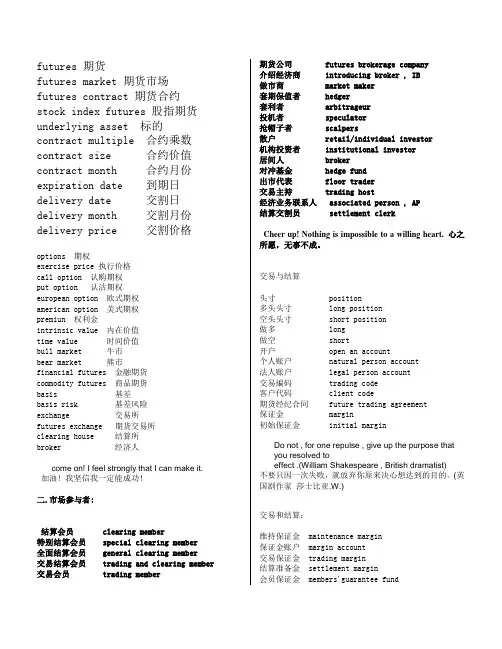
futures 期货futures market 期货市场futures contract 期货合约stock index futures 股指期货underlying asset 标的contract multiple 合约乘数contract size 合约价值contract month 合约月份expiration date 到期日delivery date 交割日delivery month 交割月份delivery price 交割价格options 期权exercise price 执行价格call option 认购期权put option 认沽期权european option 欧式期权american option 美式期权premiun 权利金intrinsic value 内在价值time value 时间价值bull market 牛市bear market 熊市financial futures 金融期货commodity futures 商品期货basis 基差basis risk 基差风险exchange 交易所futures exchange 期货交易所clearing house 结算所broker 经济人come on! I feel strongly that I can make it. 加油！我坚信我一定能成功！二.市场参与者:结算会员 clearing member特别结算会员 special clearing member全面结算会员 general clearing member交易结算会员 trading and clearing member 交易会员 trading member 期货公司 futures brokerage company介绍经济商 introducing broker , IB做市商 market maker套期保值者 hedger套利者 arbitrageur投机者 speculator抢帽子者 scalpers散户 retail/individual investor机构投资者 institutional investor居间人 broker对冲基金 hedge fund出市代表 floor trader交易主持 trading host经济业务联系人 associated person , AP结算交割员 settlement clerkCheer up! Nothing is impossible to a willing heart. 心之所愿，无事不成。

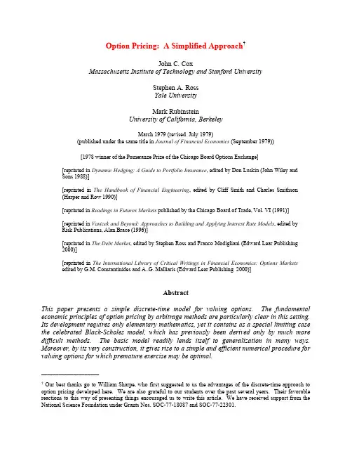
Option Pricing: A Simplified Approach†John C. CoxMassachusetts Institute of Technology and Stanford UniversityStephen A. RossYale UniversityMark RubinsteinUniversity of California, BerkeleyMarch 1979 (revised July 1979)(published under the same title in Journal of Financial Economics (September 1979))[1978 winner of the Pomeranze Prize of the Chicago Board Options Exchange][reprinted in Dynamic Hedging: A Guide to Portfolio Insurance, edited by Don Luskin (John Wiley andSons 1988)][reprinted in The Handbook of Financial Engineering, edited by Cliff Smith and Charles Smithson(Harper and Row 1990)][reprinted in Readings in Futures Markets published by the Chicago Board of Trade, Vol. VI (1991)][reprinted in Vasicek and Beyond: Approaches to Building and Applying Interest Rate Models, edited byRisk Publications, Alan Brace (1996)][reprinted in The Debt Market, edited by Stephen Ross and Franco Modigliani (Edward Lear Publishing2000)][reprinted in The International Library of Critical Writings in Financial Economics: Options Marketsedited by G.M. Constantinides and A..G. Malliaris (Edward Lear Publishing 2000)]AbstractThis paper presents a simple discrete-time model for valuing options. The fundamental economic principles of option pricing by arbitrage methods are particularly clear in this setting. Its development requires only elementary mathematics, yet it contains as a special limiting case the celebrated Black-Scholes model, which has previously been derived only by much more difficult methods. The basic model readily lends itself to generalization in many ways. Moreover, by its very construction, it gives rise to a simple and efficient numerical procedure for valuing options for which premature exercise may be optimal.____________________† Our best thanks go to William Sharpe, who first suggested to us the advantages of the discrete-time approach to option pricing developed here. We are also grateful to our students over the past several years. Their favorable reactions to this way of presenting things encouraged us to write this article. We have received support from the National Science Foundation under Grants Nos. SOC-77-18087 and SOC-77-22301.1. IntroductionAn option is a security that gives its owner the right to trade in a fixed number of shares of a specified common stock at a fixed price at any time on or before a given date. The act of making this transaction is referred to as exercising the option. The fixed price is termed the strike price, and the given date, the expiration date. A call option gives the right to buy the shares; a put option gives the right to sell the shares.Options have been traded for centuries, but they remained relatively obscure financial instruments until the introduction of a listed options exchange in 1973. Since then, options trading has enjoyed an expansion unprecedented in American securities markets.Option pricing theory has a long and illustrious history, but it also underwent a revolutionary change in 1973. At that time, Fischer Black and Myron Scholes presented the first completely satisfactory equilibrium option pricing model. In the same year, Robert Merton extended their model in several important ways. These path-breaking articles have formed the basis for many subsequent academic studies.As these studies have shown, option pricing theory is relevant to almost every area of finance. For example, virtually all corporate securities can be interpreted as portfolios of puts and calls on the assets of the firm.1 Indeed, the theory applies to a very general class of economic problems — the valuation of contracts where the outcome to each party depends on a quantifiable uncertain future event.Unfortunately, the mathematical tools employed in the Black-Scholes and Merton articles are quite advanced and have tended to obscure the underlying economics. However, thanks to a suggestion by William Sharpe, it is possible to derive the same results using only elementary mathematics.2In this article we will present a simple discrete-time option pricing formula. The fundamental economic principles of option valuation by arbitrage methods are particularly clear in this setting. Sections 2 and 3 illustrate and develop this model for a call option on a stock that pays no dividends. Section 4 shows exactly how the model can be used to lock in pure arbitrage profits if the market price of an option differs from the value given by the model. In section 5, we will show that our approach includes the Black-Scholes model as a special limiting case. By taking the limits in a different way, we will also obtain the Cox-Ross (1975) jump process model as another special case.1 To take an elementary case, consider a firm with a single liability of a homogeneous class of pure discount bonds. The stockholders then have a “call” on the assets of the firm which they can choose to exercise at the maturity date of the debt by paying its principal to the bondholders. In turn, the bonds can be interpreted as a portfolio containing a default-free loan with the same face value as the bonds and a short position in a put on the assets of the firm.2Sharpe (1978) has partially developed this approach to option pricing in his excellent new book, Investments. Rendleman and Bartter (1978) have recently independently discovered a similar formulation of the option pricing problem.Other more general option pricing problems often seem immune to reduction to a simple formula. Instead, numerical procedures must be employed to value these more complex options. Michael Brennan and Eduardo Schwartz (1977) have provided many interesting results along these lines. However, their techniques are rather complicated and are not directly related to the economic structure of the problem. Our formulation, by its very construction, leads to an alternative numerical procedure that is both simpler, and for many purposes, computationally more efficient.Section 6 introduces these numerical procedures and extends the model to include puts and calls on stocks that pay dividends. Section 7 concludes the paper by showing how the model can be generalized in other important ways and discussing its essential role in valuation by arbitrage methods.2. The Basic IdeaSuppose the current price of a stock is S = $50, and at the end of a period of time, its price must be either S* = $25 or S* = $100. A call on the stock is available with a strike price of K = $50, expiring at the end of the period.3 It is also possible to borrow and lend at a 25% rate of interest. The one piece of information left unfurnished is the current value of the call, C. However, if riskless profitable arbitrage is not possible, we can deduce from the given information alone what the value of the call must be!Consider the following levered hedge:(1) write 3 calls at C each,(2) buy 2 shares at $50 each, and(3) borrow $40 at 25%, to be paid back atthe end of the period.Table 1 gives the return from this hedge for each possible level of the stock price at expiration. Regardless of the outcome, the hedge exactly breaks even on the expiration date. Therefore, to prevent profitable riskless arbitrage, its current cost must be zero; that is,3C – 100 + 40 = 0The current value of the call must then be C = $20.3 To keep matters simple, assume for now that the stock will pay no cash dividends during the life of the call. We also ignore transaction costs, margin requirements and taxes.Table 1Arbitrage Table Illustrating the Formation of a Riskless Hedgeexpiration datepresent datewrite 3 calls 3C— –150buy 2 shares –100 50 200borrow 40 –50 –50total — —If the call were not priced at $20, a sure profit would be possible. In particular, if C = $25, the above hedge would yield a current cash inflow of $15 and would experience no further gain or loss in the future. On the other hand, if C = $15, then the same thing could be accomplished by buying 3 calls, selling short 2 shares, and lending $40.Table 1 can be interpreted as demonstrating that an appropriately levered position in stock will replicate the future returns of a call. That is, if we buy shares and borrow against them in the right proportion, we can, in effect, duplicate a pure position in calls. In view of this, it should seem less surprising that all we needed to determine the exact value of the call was its strike price, underlying stock price, range of movement in the underlying stock price, and the rate of interest. What may seem more incredible is what we do not need to know: among other things, we do not need to know the probability that the stock price will rise or fall. Bulls and bears must agree on the value of the call, relative to its underlying stock price!This example is very simple, but it shows several essential features of option pricing. And we will soon see that it is not as unrealistic as it seems.3. The Binomial Option Pricing FormulaIn this section, we will develop the framework illustrated in the example into a complete valuation method. We begin by assuming that the stock price follows a multiplicative binomial process over discrete periods. The rate of return on the stock over each period can have two possible values: u – 1 with probability q, or d – 1 with probability 1 – q. Thus, if the current stock price is S, the stock price at the end of the period will be either uS or dS. We can represent this movement with the following diagram:uS with probability qSdS with probability 1 – qWe also assume that the interest rate is constant. Individuals may borrow or lend as much as they wish at this rate. To focus on the basic issues, we will continue to assume that there are notaxes, transaction costs, or margin requirements. Hence, individuals are allowed to sell short any security and receive full use of the proceeds.4Letting r denote one plus the riskless interest rate over one period, we require u > r > d . If these inequalities did not hold, there would be profitable riskless arbitrage opportunities involving only the stock and riskless borrowing and lending.5To see how to value a call on this stock, we start with the simplest situation: the expiration date is just one period away. Let C be the current value of the call, C u be its value at the end of the period if the stock price goes to uS and C d be its value at the end of the period if the stock price goes to dS . Since there is now only one period remaining in the life of the call, we know that the terms of its contract and a rational exercise policy imply that C u = max[0, uS – K ] and C d = max[0, dS – K ]. Therefore,Cu = max[0, uS – K ] with probability qCC d = max[0, dS – K ] with probability 1 – qSuppose we form a portfolio containing Δ shares of stock and the dollar amount B in riskless bonds.6 This will cost ΔS + B . At the end of the period, the value of this portfolio will beΔuS + rB with probability qΔS + BΔdS + rB with probability 1 – qSince we can select Δ and B in any way we wish, suppose we choose them to equate the end-of-period values of the portfolio and the call for each possible outcome. This requires thatΔuS + rB = C uΔdS + rB = C dSolving these equations, we findrd u dC uC B S d u C C u d d u )(,)(!!=!!=" (1)4 Of course, restitution is required for payouts made to securities held short.5 We will ignore the uninteresting special case where q is zero or one and u = d = r .6 Buying bonds is the same as lending; selling them is the same as borrowing.With Δ and B chosen in this way, we will call this the hedging portfolio.If there are to be no riskless arbitrage opportunities, the current value of the call, C , cannot be less than the current value of the hedging portfolio, ΔS + B . If it were, we could make a riskless profit with no net investment by buying the call and selling the portfolio. It is tempting to say that it also cannot be worth more, since then we would have a riskless arbitrage opportunity by reversing our procedure and selling the call and buying the portfolio. But this overlooks the fact that the person who bought the call we sold has the right to exercise it immediately.Suppose that ΔS + B < S – K . If we try to make an arbitrage profit by selling calls for more than ΔS + B , but less than S – K , then we will soon find that we are the source of arbitrage profits rather than the recipient. Anyone could make an arbitrage profit by buying our calls and exercising them immediately.We might hope that we will be spared this embarrassment because everyone will somehow find it advantageous to hold the calls for one more period as an investment rather than take a quick profit by exercising them immediately. But each person will reason in the following way. If I do not exercise now, I will receive the same payoff as a portfolio with ΔS in stock and B in bonds. If I do exercise now, I can take the proceeds, S – K , buy this same portfolio and some extra bonds as well, and have a higher payoff in every possible circumstance. Consequently, no one would be willing to hold the calls for one more period.Summing up all of this, we conclude that if there are to be no riskless arbitrage opportunities, it must be true thatB SC +!=r d u dC uC d u C C u d d u )(!!+!!=r C d u r u C d u d r d u /!"#$%&'()*+,--+'()*+,--= (2)if this value is greater than S – K , and if not, C = S – K .7Equation (2) can be simplified by definingd u d r p !!" and du r u p !!"!1 so that we can writeC = [pC u + (1 – p )C d ]/r (3)It is easy to see that in the present case, with no dividends, this will always be greater than S – K as long as the interest rate is positive. To avoid spending time on the unimportant situations where the interest rate is less than or equal to zero, we will now assume that r is always greater 7 In some applications of the theory to other areas, it is useful to consider options that can be exercised only on the expiration date. These are usually termed European options. Those that can be exercised at any earlier time as well, such as we have been examining here, are then referred to as American options. Our discussion could be easily modified to include European calls. Since immediate exercise is then precluded, their values would always be given by (2), even if this is less than S – K .than one. Hence, (3) is the exact formula for the value of a call one period prior to the expiration in terms of S, K, u, d, and r.To confirm this, note that if uS ≤K, then S < K and C = 0, so C > S – K. Also, if dS ≥K, then C = S – (K/r) > S – K. The remaining possibility is uS > K > dS. In this case, C = p(uS – K)/r. This is greater than S – K if (1 – p)dS > (p – r)K, which is certainly true as long as r > 1.This formula has a number of notable features. First, the probability q does not appear in the formula. This means, surprisingly, that even if different investors have different subjective probabilities about an upward or downward movement in the stock, they could still agree on the relationship of C to S, u, d, and r.Second, the value of the call does not depend on investors’ attitudes toward risk. In constructing the formula, the only assumption we made about an individual’s behavior was that he prefers more wealth to less wealth and therefore has an incentive to take advantage of profitable riskless arbitrage opportunities. We would obtain the same formula whether investors are risk-averse or risk-preferring.Third, the only random variable on which the call value depends is the stock price itself. In particular, it does not depend on the random prices of other securities or portfolios, such as the market portfolio containing all securities in the economy. If another pricing formula involving other variables was submitted as giving equilibrium market prices, we could immediately show that it was incorrect by using our formula to make riskless arbitrage profits while trading at those prices.It is easier to understand these features if it is remembered that the formula is only a relative pricing relationship giving C in terms of S, u, d, and r. Investors’ attitudes toward risk and the characteristics of other assets may indeed influence call values indirectly, through their effect on these variables, but they will not be separate determinants of call value.Finally, observe that p ≡ (r – d)/(u – d) is always greater than zero and less than one, so it has the properties of a probability. In fact, p is the value q would have in equilibrium if investors were risk-neutral. To see this, note that the expected rate of return on the stock would then be the riskless interest rate, soq(uS) + (1 – q)(dS) = rSandq = (r – d)/(u – d) = pHence, the value of the call can be interpreted as the expectation of its discounted future value in a risk-neutral world. In light of our earlier observations, this is not surprising. Since the formula does not involve q or any measure of attitudes toward risk, then it must be the same for any set of preferences, including risk neutrality.It is important to note that this does not imply that the equilibrium expected rate of return on the call is the riskless interest rate. Indeed, our argument has shown that, in equilibrium, holding the call over the period is exactly equivalent to holding the hedging portfolio. Consequently, the riskand expected rate of return of the call must be the same as that of the hedging portfolio. It can be shown that Δ≥ 0 and B ≤ 0, so the hedging portfolio is equivalent to a particular levered long position in the stock. In equilibrium, the same is true for the call. Of course, if the call is currently mispriced, its risk and expected return over the period will differ from that of the hedging portfolio.Now we can consider the next simplest situation: a call with two periods remaining before its expiration date. In keeping with the binomial process, the stock can take on three possible values after two periods,u2SuSS duSdSd2SSimilarly, for the call,C uu = max[0, u2S – K]C uC C du = max[0, duS – K]C dC dd = max[0, d2S – K]C uu stands for the value of a call two periods from the current time if the stock price moves upward each period; C du and C dd have analogous definitions.At the end of the current period there will be one period left in the life of the call, and we will be faced with a problem identical to the one we just solved. Thus, from our previous analysis, we know that when there are two periods left,C u = [pC uu + (1 – p)C ud]/rand (4)C d = [pC du + (1 – p)C dd]/rAgain, we can select a portfolio with ΔS in stock and B in bonds whose end-of-period value will be C u if the stock price goes to uS and C d if the stock price goes to dS. Indeed, thefunctional form of Δ and B remains unchanged. To get the new values of Δ and B, we simply use equation (1) with the new values of C u and C d.Can we now say, as before, that an opportunity for profitable riskless arbitrage will be available if the current price of the call is not equal to the new value of this portfolio or S – K, whichever is greater? Yes, but there is an important difference. With one period to go, we could plan to lock in a riskless profit by selling an overpriced call and using part of the proceeds to buy the hedging portfolio. At the end of the period, we knew that the market price of the call must be equal to the value of the portfolio, so the entire position could be safely liquidated at that point. But this was true only because the end of the period was the expiration date. Now we have no such guarantee. At the end of the current period, when there is still one period left, the market price of the call could still be in disequilibrium and be greater than the value of the hedging portfolio. If we closed out the position then, selling the portfolio and repurchasing the call, we could suffer a loss that would more than offset our original profit. However, we could always avoid this loss by maintaining the portfolio for one more period. The value of the portfolio at the end of the current period will always be exactly sufficient to purchase the portfolio we would want to hold over the last period. In effect, we would have to readjust the proportions in the hedging portfolio, but we would not have to put up any more money.Consequently, we conclude that even with two periods to go, there is a strategy we could follow which would guarantee riskless profits with no net investment if the current market price of a call differs from the maximum of ΔS + B and S – K. Hence, the larger of these is the current value of the call.Since Δ and B have the same functional form in each period, the current value of the call in terms of C u and C d will again be C = [pC u + (1 – p)C d]/r if this is greater than S – K, and C = S – K otherwise. By substituting from equation (4) into the former expression, and noting that C du = C ud, we obtainC = [p2C uu + 2p(1 – p)C ud + (1 – p)2C dd]/r2(5)= [p2max[0, u2S – K] + 2p(1 – p)max[0, duS – K] + (1 – p)2max[0, d2S – K]]/r2A little algebra shows that this is always greater than S – K if, as assumed, r is always greater than one, so this expression gives the exact value of the call.8All of the observations made about formula (3) also apply to formula (5), except that the number of periods remaining until expiration, n, now emerges clearly as an additional determinant of the call value. For formula (5), n = 2. That is, the full list of variables determining C is S, K, n, u, d, and r.8 In the current situation, with no dividends, we can show by a simple direct argument that if there are no arbitrage opportunities, then the call value must always be greater than S – K before the expiration date. Suppose that the call is selling for S –K. Then there would be an easy arbitrage strategy that would require no initial investment and would always have a positive return. All we would have to do is buy the call, short the stock, and invest K dollars in bonds. See Merton (1973). In the general case, with dividends, such an argument is no longer valid, and we must use the procedure of checking every period.We now have a recursive procedure for finding the value of a call with any number of periods to go. By starting at the expiration date and working backwards, we can write down the general valuation formula for any n :n j n j j n j n j r K S d u p p j n j n C /],0max[)1()!(!!0!!"#$$%&''(()*++,-'=''=. (6)This gives us the complete formula, but with a little additional effort we can express it in a more convenient way.Let a stand for the minimum number of upward moves that the stock must make over the next n periods for the call to finish in-the-money. Thus a will be the smallest non-negative integer such that u a d n-a S > K . By taking the natural logarithm of both sides of this inequality, we could write a as the smallest non-negative integer greater than log(K /Sd n )/log(u /d ).For all j < a ,max[0, u j d n-j S – K ] = 0and for all j ≥ a ,max[0, u j d n-j S – K ] = u j d n-j S – K Therefore,n j n j j n j n a j r K S d u p p j n j n C /][)1()!(!!!"#$%&''(()*++,-'=''=.Of course, if a > n , the call will finish out-of-the-money even if the stock moves upward every period, so its current value must be zero.By breaking up C into two terms, we can write!!"#$$%&''()**+,-''()**+,-=--=.n j n j j n j n a j r d u p p j n j n S C )1()!(!!!"#$%&'(()*++,-'''='.j n j n a j n p p j n j n Kr )1()!(!!Now, the latter bracketed expression is the complementary binomial distribution function φ[a ; n , p ]. The first bracketed expression can also be interpreted as a complementary binomial distribution function φ[a ; n , p ′], wherep ′ ≡ (u /r )p and 1 – p ′ ≡ (d /r )(1 – p )p ′ is a probability, since 0 < p ′ < 1. To see this, note that p < (r /u ) andj n j j n j n j n j j n j p p p r d p r u r d u p p !!!!"!"=#$%&'(!=#$%&'(=))*+,,-.!)1()1()1(In summary:Binomial Option Pricing FormulaC = Sφ[a; n, p′] – Kr–nφ[a; n, p]wherep ≡ (r – d)/(u – d) and p′≡ (u/r)pa ≡ the smallest non-negative integergreater than log(K/Sd n)/log(u/d)If a > n, then C = 0.It is now clear that all of the comments we made about the one period valuation formula are valid for any number of periods. In particular, the value of a call should be the expectation, in a risk-neutral world, of the discounted value of the payoff it will receive. In fact, that is exactly what equation (6) says. Why, then, should we waste time with the recursive procedure when we can write down the answer in one direct step? The reason is that while this one-step approach is always technically correct, it is really useful only if we know in advance the circumstances in which a rational individual would prefer to exercise the call before the expiration date. If we do not know this, we have no way to compute the required expectation. In the present example, a call on a stock paying no dividends, it happens that we can determine this information from other sources: the call should never be exercised before the expiration date. As we will see in section 6, with puts or with calls on stocks that pay dividends, we will not be so lucky. Finding the optimal exercise strategy will be an integral part of the valuation problem. The full recursive procedure will then be necessary.For some readers, an alternative “complete markets” interpretation of our binomial approach may be instructive. Suppose that πu and πd represent the state-contingent discount rates to states u and d, respectively. Therefore, πu would be the current price of one dollar received at the end of the period, if and only if state u occurs. Each security — a riskless bond, the stock, and the option — must all have returns discounted to the present by πu and πd if no riskless arbitrage opportunities are available. Therefore,1 = πu r + πd rS = πu(uS) + πd(dS)C = πu C u + πd C dThe first two equations, for the bond and the stock, implyr d u d r u 1!"#$%&''=( and rd u r u d 1!"#$%&''=(Substituting these equalities for the state-contingent prices in the last equation for the option yields equation (3).It is important to realize that we are not assuming that the riskless bond and the stock and the option are the only three securities in the economy, or that other securities must follow a binomial process. Rather, however these securities are priced in relation to others in equilibrium, among themselves they must conform to the above relationships.From either the hedging or complete markets approaches, it should be clear that three-state or trinomial stock price movements will not lead to an option pricing formula based solely on arbitrage considerations. Suppose, for example, that over each period the stock price could move to uS or dS or remain the same at S . A choice of Δ and B that would equate the returns in two states could not in the third. That is, a riskless arbitrage position could not be taken. Under the complete markets interpretation, with three equations in now three unknown state-contingent prices, we would lack the redundant equation necessary to price one security in terms of the other two.4. Riskless Trading StrategiesThe following numerical example illustrates how we could use the formula if the current market price M ever diverged from its formula value C . If M > C , we would hedge, and if M < C , “reverse hedge”, to try and lock in a profit. Suppose the values of the underlying variables areS = 80, n = 3, K = 80, u = 1.5, d = 0.5, r = 1.1In this case, p = (r – d )/(u – d ) = 0.6. The relevant values of the discount factor arer -1 = 0.909, r -2 = 0.826, r -3 = 0.751The paths the stock price may follow and their corresponding probabilities (using probability p ) are, when n = 3, with S – 80,。

capm模型的名词解释投资领域中的CAPM模型被广泛用于衡量风险和回报的关系。

CAPM是英文名称Capital Asset Pricing Model的缩写，中文翻译为资本资产定价模型。

它是由美国经济学家沃伦·巴菲特在1964年首次提出的。

本文将对CAPM模型涉及的一些名词进行解释和探讨，以便更好地理解这一模型。

1. 资本资产定价模型（Capital Asset Pricing Model）资本资产定价模型是一个衡量资本资产收益与风险之间关系的理论模型。

它的核心概念是用回报率的期望值和风险的标准差来衡量资产的预期收益率。

CAPM模型认为，一个资产的回报率应该等于无风险回报率与该资产的风险系数（β）的乘积，再加上市场整体回报率减去无风险回报率的差异。

2. 无风险回报率（Risk-Free Rate）无风险回报率是投资者可以在完全没有风险的情况下获得的回报率，比如国家债券或其他政府支持的债券。

CAPM模型使用无风险回报率作为市场的参考点，因为投资者应该至少要得到与无风险投资相当的回报。

3. β系数（Beta）β系数衡量了一个资产相对于整个市场波动的程度。

它是资产的系统性风险，也称为市场风险。

β系数的计算基于历史数据，通过与市场整体的回报率进行对比，可以获得一个资产的β系数。

β系数大于1表示资产的波动比市场整体更大，而小于1则表示资产的波动比市场整体更小。

4. 风险溢价（Risk Premium）风险溢价表示投资者因承担更高风险而获得的额外回报。

在CAPM模型中，风险溢价是指资产预期回报率与无风险回报率之间的差异。

投资者愿意承担更高的风险，是因为他们期望通过获得更高的回报来弥补这种风险。

5. 市场整体回报率（Market Return）市场整体回报率是指整个市场内所有资产组合的回报率加权平均值。

在CAPM 模型中，市场整体回报率也被称为市场组合回报率，它是根据市场上所有资产的权重来计算的。

市场整体回报率的变化将直接影响资产的期望回报率。