星载毫米波测云雷达资料的云特征分析

分布式星载雷达回波特性分析与仿真的开题报告一、选题背景随着卫星技术的不断发展和应用，卫星遥感领域也得到了快速发展。

卫星雷达遥感是传统遥感技术中比较重要的技术之一，其在地球观测、自然资源调查和环境监测等方面有着重要的应用。

卫星雷达遥感不仅可以获取高质量、高分辨率的数据，还具有高度的不受云层和天气限制、全天候观测能力等优点，因此被广泛应用于地震、海洋、气象、城市规划等领域。

分布式星载雷达具有多发射机、多接收机的特点，可以实现高精度的成像和数据处理，因此在卫星雷达领域也有着广泛的应用前景。

二、研究目的和意义本研究旨在分析分布式星载雷达回波特性，并通过仿真方法对其成像效果进行评估。

具体目的如下：1.通过对分布式星载雷达回波信号特性的分析，研究其成像效果的影响因素。

2.建立分布式星载雷达仿真模型，评估其成像效果。

3.对比分析传统单发射机、单接收机卫星雷达与分布式星载雷达的成像效果，探讨分布式星载雷达的优势和应用前景。

三、研究内容和方法本研究将分为以下两个部分：1.回波特性分析通过分析分布式星载雷达回波信号的特性，包括目标回波功率、功率谱密度、多普勒频率谱、角分辨率等，研究其成像效果的影响因素。

2.仿真模型建立和成像效果评估在MATLAB软件中建立分布式星载雷达仿真模型，模拟目标回波信号的生成和接收。

通过对仿真数据的处理和成像算法的分析，评估分布式星载雷达的成像效果。

与传统单发射机、单接收机卫星雷达进行对比分析，探讨分布式星载雷达的优势和应用前景。

四、预期成果本研究的预期成果包括以下几个方面：1.分析分布式星载雷达回波信号特性，研究其成像效果的影响因素。

2.建立分布式星载雷达仿真模型，评估其成像效果。

3.与传统单发射机、单接收机卫星雷达进行对比分析，探讨分布式星载雷达的优势和应用前景。

4.完成科研论文一篇，为卫星雷达遥感领域的发展做出贡献。

五、论文结构本论文将由以下几个部分组成：1.绪论：介绍分布式星载雷达的背景和研究意义，对相关研究进行回顾和分析。

雷达回波和卫星云图观测夜间云浅析作者：暂无来源：《农民致富之友（上半月）》 2014年第6期杨海龙钱继成摘要：通过卫星云图图象的形态、结构、亮度和纹理等特征，可以识别云的种、属及降水状况。

可以识别大范围的云系，如螺旋状、带状、逗点状、波状、细胞状等，并用以推断锋面、温带气旋、热带风暴，高空急流等大尺度天气系统的位置和特征。

根据晴空无云的区域，推断反气旋和高空高压脊的位置。

从卫星云图上发现了一些新的云系；如细胞状云系、云街、热带云团等。

利用云状在卫星云图、多普勒雷达图中的外形、结构和图像特征，归纳了若干利用卫星云图和多普勒雷达图像在夜间云观测中应用的一些方法。

如卫星云图上积雨云常呈球形或胡萝卜形；高层云和高积云为层状；卷云为纤维状等特点。

雷达图上雨层云为分片成片、面积大和回波在20dBz左右，积雨云为结构紧密、棱角分明、回波强度大等特点。

关键词：大气探测；夜间云观测；卫星云图；雷达图像云状最能从空间反映某处特定时问的天气状况，云状观测是地面气象观测中的重要组成部分，也是难度较大的目测项目。

特别是在夜间，由于光照不足，观测员难以像白天那样清楚地看见天上云的外部和分布特征，容易出现一些失真和疑误记录。

因此，除了熟练掌握夜间云的特征进行观测外，还可利用卫星云图、多普勒雷达图像夜间云的特点，为提高观测的准确性提供更多保障。

本文归纳了一些从地面观测到的云在卫星云图和雷达图像上的特点。

1卫星云图上云的特征在卫星云图上，根据云的外形分成3个主要类别：积状云(积云、浓积云、积雨云、层积云)，层状云(厚的雾、层云、高层云、高积云、雨层云)和卷状云(毛卷云、密卷云、卷层云)。

1)积状云：主要反映了大气不稳定度变化的程度，对它们的识别是通过带状、细胞状或波状云型以及由形状不规则云素的大小变化来实现。

积云较小，常以微小的斑迹出现，比无云的时候较亮。

浓积云常呈现形状不规则的云素或云素群。

积雨云云体浓厚庞大，垂直发展旺盛，呈现球形或胡萝卜形。

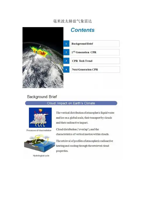
毫米波太赫兹气象雷达
简介：CPR（Cloud Profiling Radar)主要用于地球环境监测并着重监控云上升和下降的动态信息、云粒和气溶胶生成以及保有状况等信息。

由于云层由微小水滴或冰颗粒组成，比雨滴直径要小的多，所以对云层以及体积更小的气溶胶探测需要毫米波雷达来实现。

94GHz测云雷达甚至可以”切开”云层获得云层的垂直剖面结构特征从而使气象学家可以获得云层的三维照片。

2006年NASA发射的CloudSAT成功证明了CPR的有效性，两年后即将升空的EarthCare卫星将提供更高的灵敏度和更好的分辨率。

在欧洲和中国，下一代的星载220GHz CPR均处于原型机阶段，它将帮助气象学家分辨出更小的雨滴以及雪花的内部结构，改善现有NWP（数值气象预测）模型。

同时随着太赫兹放大器技术的发展，固态放大器很快将实现200GHz/1W的输出功率，真空器件EIK、TWT放大器也将有长足发展。

分辨率更高，灵敏度更高的CPR 即将成为现实。

毫米波在雾和云中的衰减特性分析Ξ王　威　李进杰　高　伟　顾德均(海军航空工程学院青岛分院　青岛266041)【摘要】　主要讨论了毫米波在雾和云中的传播特性及受到的影响.并通过毫米波雷达性能模型,模拟出了毫米波回波的性能曲线。

【关键词】　毫米波,传播,回波T he P rop agati on Character of M illi m eter W ave in Fog and C loudW ANGW e i　L I J i n-j ie　GAO W e i　GU D e-jun(N aval A eronau tical Engineering A cadem y Q ingdao B ranch　Q ingdao266041)【Abstract】　T h is paper discu sses the p ropagati on character of m illi m eter w ave in fog and cloud.Con sidering the real circum stance,w ith m athem atical model,w e draw som e common conclu si on.【Key words】　m illi m eter w ave,p ropagati on,echo w ave1　概述毫米波技术的应用是当今重要的军事应用之一,由于毫米波制导系统能在恶劣气象条件下和战场烟幕条件下工作,且设备尺寸较小,所以目前毫米波制导系统得到了广泛的应用。

但是在坏天气下毫米波的作用距离下降。

本文主要分析雾和云对毫米波制导系统的影响。

2　雷达方程的修正在不考虑大气及恶劣天气(如雨、雾)影响的条件下,雷达方程可以写成S N=P t G2Κ2ΡT(4Π)3R4L ikT0B n F n(1)式中P t—发射功率(W),G—天线增益,Κ—雷达工作波长,R—弹目距离,ΡT—目标的有效雷达截面, S N—接收信噪比,L i—系统的插入损耗,B n—接收机带宽,F n—接收机噪声系数,k—玻尔兹曼常数为1.38×10-23J K,T0—雷达工作温度(K)。

基于毫米波云雷达的伊犁河谷两次强降雪过程云特征观测分析张晋茹; 杨莲梅【期刊名称】《《沙漠与绿洲气象》》【年(卷),期】2019(013)005【总页数】8页(P41-48)【关键词】毫米波云雷达; 伊犁河谷; 强降雪; 反射率因子; 径向速度【作者】张晋茹; 杨莲梅【作者单位】中国气象局乌鲁木齐沙漠气象研究所新疆乌鲁木齐830002; 中亚大气科学研究中心新疆乌鲁木齐830002【正文语种】中文【中图分类】P426.5新疆是干旱半干旱气候，但由于三山夹两盆的特殊地形，特别是在冬季新疆北部，极锋急流频繁南下，新疆是中国冬季降雪最多、积雪最丰富的三大区域之一[1]，许多学者从大尺度环流背景、天气尺度和中尺度系统、水汽特征等方面对新疆降雪进行了研究[2-10]。

也有不少研究人员应用卫星资料对新疆地区非降水云和降水云宏微观物理特性进行了研究[11-16]。

但卫星资料的时空分辨率低，穿透云的能力限制，不能对降雪过程进行一次完整的观测。

毫米波云雷达具有很高的灵敏度和时空分辨率，能够探测晴空云微小粒子结构和微物理特性，也还能够对弱降水和降雪系统宏观结构观测和微物理参数的反演[17]。

陈羿辰等[17]利用毫米波云雷达对降雪系统进行观测分析，结果表明降雪发展旺盛时期雪粒子含水量在0.05～0.15 g/m3。

王柳柳等[18]利用云雷达进行冻雨—降雪微物理和动力特征分析，结果表明冻雨和降雪过程初始时期形成的平均粒子半径分别在40 μm和120 μm 附近。

王德旺等[19]利用偏振云雷达、雨滴谱仪和探空联合观测一次混合型层状云降水得到在较强回波区，云水含量为0.5～0.8 g/kg，雨水含量为0.2 g/kg，空气垂直速度为0.6～1.0 m/s。

李海飞等[20]利用云雷达对淮南冬季云宏观特性进行研究，该地区冬季云底高度在0.21～11.0 km，云顶分布在0.36～11.3 km，云厚度为0.1～8.3 km。

伊犁河谷位于新疆西部，是新疆乃至全国天气系统的上游，对下游地区天气系统具有较强的指示意义，同时伊犁河谷也是全疆的降水中心[21]，新源是伊犁河谷地区具有代表性的降水区域。

毫米波测云雷达的设计与应用的开题报告开题报告：毫米波测云雷达的设计与应用一、选题背景与意义毫米波测云雷达是一种能够测量大气云层内水滴和晶体的粒子性质的仪器。

它主要利用毫米波辐射在云粒子上所引起的散射反射特性，通过接受和处理反射回来的信号得到相应的反演产品。

毫米波测云雷达作为一种非常重要的气象仪器，广泛应用于气象探测、空气污染和大气环境监测等领域。

随着气象科学及相关领域的不断发展，传统的毫米波测云雷达已经难以满足现代科学研究和应用的需要。

为此，需要设计一种新型的毫米波测云雷达，能够提高反演精度和性能，满足实际应用需要。

二、研究目的本研究的目的是设计一种新型的毫米波测云雷达，能够提高反演精度和性能，满足实际应用需要。

三、研究内容本研究的主要内容包括：1.毫米波测云雷达的原理及成像算法研究2.毫米波测云雷达的硬件设计和软件开发3.毫米波测云雷达的反演实验及性能分析四、研究方法本研究将采用以下研究方法：1.文献调研法：对毫米波测云雷达的相关研究成果、技术方案及应用现状进行系统梳理和分析。

2.仿真模拟法：通过建立毫米波测云雷达的数学模型，进行理论仿真和实验验证。

3.实验研究法：通过在实验平台上进行毫米波测云雷达性能评估和反演实验，获得实际数据并进行分析。

五、预期成果本研究的预期成果包括：1.设计出一种能够提高反演精度和性能的新型毫米波测云雷达。

2.掌握毫米波测云雷达的原理和成像算法。

3.验证新型毫米波测云雷达的性能，并与传统毫米波测云雷达进行比较。

六、研究难点及解决方案本研究的难点在于如何提高毫米波测云雷达的反演精度和性能。

针对这一难点，可以尝试采用以下解决方案：1.采用先进的硬件设计和软件开发技术，提高毫米波测云雷达的信噪比和分辨率。

2.引入新的成像算法，提高毫米波测云雷达的反演精度和性能。

3.通过实验研究和数据分析，优化毫米波测云雷达的性能和参数设置。

七、进度安排1.第一年：完成毫米波测云雷达原理及成像算法研究，并进行硬件设计和软件开发。

引言云降水微物理和动力特征的探测对于理解降水的形成和发展、降水系统和周边环境的相互作用、云系对大气辐射影响、检验和验证数值模式云降水参数化方案和云降水模拟能力有非常重要的作用。

地面的雨滴谱可以通过雨滴谱仪进行直接观测，空中的云降水参数可以通过飞机进行直接观测，但飞机很难获取云降水参数的连续时空分布，特别是对流系统内的上升速度、滴谱等观测更加困难。

气象雷达通过主动遥感方式，可以获取到云降水的回波强度、径向速度和速度谱宽等参数的三维分布的连续变化，在一定假设情况下，得到雨滴谱参数和风场等三维分布。

通常雨滴谱反演分为两类，第一类是假定雨滴谱的分布特征来反演雨滴谱参数，如指数分布反演两个参数，Gamma 分布反演三个参数，这包括双线偏振雷达反演雨滴谱参数、利用双波段云雷达回波强度差反演雨滴谱参数等方法；第二类是直接反演雨滴谱分布，这种方法必须基于垂直观测的多普勒功率谱数据。

云和降水虽然是紧密联系的，但因粒子大小差别很大，而后向散射能力与粒子尺度的六次方成正比(瑞利散射条件下)，所以云的回波强度要远远小于降水。

探测云的云雷达(采用毫米波)与探测降水的天气雷达(采用厘米波)在雷达最小可测回波强度、波长、扫描方式等方面有很大的差别。

最小可测回波强度是云雷达一个非常重要的指标，云雷达通常采用短波长和脉冲压缩刘黎平.2021.毫米波云雷达观测和反演云降水微物理及动力参数方法研究进展[J].暴雨灾害,40(3):231-242LIU Liping.2021.Reviews on retrieval methods for microphysical and dynamic parameters with cloud radar [J].Torrential Rain and Disas-ters,40(3):231-242毫米波云雷达观测和反演云降水微物理及动力参数方法研究进展刘黎平(中国气象科学研究院灾害天气国家重点实验室，北京100081)摘要：云雷达是探测和反演云降水微物理及动力参数精细结构的重要手段。

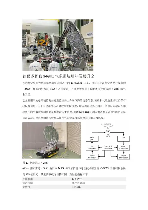
首套多普勒94GHz气象雷达明年发射升空
作为欧空局七大地球探测卫星计划之一的EarthCARE卫星，由日本宇宙航空研究开发机构（JAXA）和欧洲航天局（ESA）共同研制，并且是世界上首颗配备多普勒雷达（CPR）的气象卫星。

它主要用于地球环境监测并着重监控云上升和下降的动态信息、云粒和气溶胶生成以及保有状况等信息。

由于云层由微小水滴或冰颗粒组成，比雨滴直径要小的多，所以对云层以及体积更小的气溶胶探测需要毫米波雷达来实现。

其搭载的94GHz测云雷达甚至可以”切开”云层获得云层的垂直剖面结构特征从而使气象学家可以获得云层的三维照片。

图1：测云雷达（CPR）
94GHz测云雷达（CPR）由日本JAXA和国家信息与通信技术研究所（NICT）开发研制总耗资135亿日元。

其主要系统内结构如图1及性能指标如下:
工作频率94.05GHz
雷达机制脉冲多普勒
灵敏度>-35dBz
发射功率、脉宽及重复频率 1.5KW(EIK)/3.3us/ 6100~7500 Hz
主反射面天线 2.5m(碳纤维复合材料)
卫星高度400km
分辨率500m
多普勒精度<1m/s
波束宽度0.095 deg
这是继2006年NASA和加拿大航天局合作的CloudSat卫星后第二颗携带94GHz测云雷达的气象卫星。

最初预计在2012年发射升空，经过多次延期后最终计划于2018年在库鲁航天中心发射。

随着高频率放大器、隔离器等器件的成熟，越来越多的毫米波以及太赫兹气象雷达将为大气探测服务。

图2：英国TK公司为CPR提供的准光环形器实物图
图3：加拿大CPI公司提供的94GHz功率放大器EIK。

ARM TR-018 Millimeter Wave Cloud Radar (MMCR)HandbookJanuary 2005K. B. WidenerK. JohnsonWork supported by the U.S. Department of Energy,Office of Science, Office of Biological and Environmental ResearchContents1.General Overview (1)2.Contacts (1)3.Deployment Locations and History (1)4.Near-Real-Time Data Plots (2)5.Data Description and Examples (3)6.Data Quality (2)7.Instrument Details (3)FiguresFigure 1 (7)Figure 2 (8)TablesTable 1. MMCR Deployment Locations and Dates (1)Table 2. MMCR Data Stream Availability (3)Table 3. Primary Variables (3)Table 4. Secondary Variables (4)Table 6. Dimension Variables (6)Table 7. ARM SGP Site Operation Parameters 1997.09.15 – 2004.08.10 (5)Table 8. Calibration Information (6)Table 9. MMCR Antenna Table (7)1. General OverviewThe millimeter cloud radar (MMCR) systems probe the extent and composition of clouds at millimeter wavelengths. The MMCR is a zenith-pointing radar that operates at a frequency of 35 GHz. The main purpose of this radar is to determine cloud boundaries (e.g., cloud bottoms and tops). This radar will also report radar reflectivity (dBZ) of the atmosphere up to 20 km. The radar possesses a doppler capability that will allow the measurement of cloud constituent vertical velocities.2. Contacts2.1 MentorKevin WidenerPacific Northwest National LaboratoryP.O. Box 999Richland, WA 99352Phone: 509-375-2487Fax: 509-375-6736kevin.widener@Karen JohnsonEnvironmental Sciences DepartmentBrookhaven National LaboratoryUpton, NY 11973Phone: 631-344-5952Fax: 631-344-2060kjohnson@2.2 Instrument DeveloperKen Moran, Project LeaderNOAA Environmental Research LaboratoriesEnvironmental Technology Laboratory325 Broadway, R/E/ET4Boulder, CO 80303Phone: 303- 497-6575Ken.Moran@3. Deployment Locations and HistoryTable 1. MMCR Deployment Locations and DatesLocation Date Installed Date Removed StatusSGP/C1 1996/11/08 OperationalNSA/C1 1998/03/25 OperationalTWP/C1 1999/06/14 OperationalTable 1. (cont’d)Location Date Installed Date Removed StatusTWP/C2 1998/10/22 OperationalTWP/C3 2002/03/06 OperationalThe first five MMCRs were built by the National Oceanic and Atmospheric Administration’s (NOAA’s) Environment Technology Laboratory (ETL) in Boulder, Colorado. The first unit is now operating at the Southern Great Plains (SGP) Central Facility. The second unit is currently operating at the North Slope of Alaska/Adjacent Artic Ocean (NSA/AAO) site, and the third and forth units are located at the Tropical Western Pacific’s Atmospheric Radiation and Cloud Station (TWP’s ARCS-1) on Manus Island and ARCS-2 on Nauru Island. The fifth unit is a hot spare/development radar located at NOAA/ETL. The sixth radar was built by Radian International; it is currently installed at Darwin, Northern Territory, Australia at the ARCS-3 site.In addition to the ARM MMCRs, NOAA/ETL fielded an identical radar during the Surface Heat Budget of the Arctic Ocean (SHEBA) () experiment from the fall of 1997 to the fall of 1998.A new MMCR data processor, the C-40, was developed by NOAA/ETL and installed at the SGP and NSA sites in September 2003 and April 2004, respectively. Along with the new MMCR radar computer, the C-40 provides faster data collection and much improved instrument reliability. Upgrades are planned for the TWP sites in the coming year.4. Near-Real-Time Data PlotsNear-real-time MMCR data plots are available from the Data Quality Office (DQO) for each site. Thumbnail images of the most recent data are available from the ARM DQHandS Plot Browser website. Select the site of interest and select the associated MMCR data stream. For NSA, choose‘nsammcrmom,’ for SGP select ‘sgpmmcrmom,’ and for the TWP sites, select ‘twpmmcrcal.’ Then choose either the ‘list’ or ‘thumbnail’ search option. The ‘list’ option provides a list of available plots; the ‘thumbnail’ option presents thumbnails images. The most recent week of data is the default date range.DQO plots can also be accessed individually via /PLOTS. MMCR plots for each site are accessible as listed below. In each case, select the date of interest from the page that appears: NSA: /PLOTS/NSA/nsammcrmom/SGP: /PLOTS/SGP/sgpmmcrmom/TWP: /PLOTS/TWP/twpmmcrcal/(Individual TWP site plots for C1, C2 are accessible once a date is selected. Plots for TWP-C3 are not yet available from the DQO.)5. Data Description and ExamplesMMCR data are available from the ARM Data Archive in the following data streams: mmcrmom,mmcrcal, mmcrmoments, and mmcrspecmom. This table indicates which data streams are available ateach site and time period:Table 2.MMCR Data Stream AvailabilityDate RangeSitemmcrcal, mmcrmoments mmcrmomNSA 1999.03 - 2004.04.12 2004.04.13 - PresentSGP 1996.11 - 2003.09.08 2003.09.09 - PresentTWP-C1 1999.08 - PresentTWP-C2 1998.11 - PresentTWP-C3 2002.03 - PresentThe data streams ‘mmcrcal’ and ‘mmcrmoments’ together make up a complete set of MMCR data.The ‘mmcrmom’ data stream alone contains all the MMCR data fields.5.1 Data File Contents5.1.1 Primary Variables and Expected UncertaintyThe following tables show the primary quantities measured by the MMCR for the mmcrmom data stream,followed by the mmcrcal, mmcrmoments data streams.Table 3. Primary Variablesmmcrmom Data Stream (current SGP, NSA)Uncertainty Variable DescriptionReflectivity MMCR Reflectivity (time, height), in dBZ 0.5dBMeanDopplerVelocity MMCR Mean Doppler Velocity (time, height), in m/s 0.1 m/sSpectralWidth MMCR Spectral Width (time, height), in m/s 0.1 m/sCircularDepolarizationRatio MMCR Circular Depolarization Ratio (time, height), dBmmcrcal / mmcrmoments Data Streams (current TWP, historical SGP, NSA)Stream Description Uncertainty Variable DataReflectivity mmcrcal MMCR Reflectivity (time-height), in dBZ 0.5 dBMeanDopplerVelocity mmcrmoments MMCR Mean Doppler Velocity (time-height), in0.1 m/sm/sSpectralWidth mmcrmoments MMCR Spectral Width (time, height), in m/s 0.1 m/sThe overall uncertainties for the primary quantities measured are as follows:•Measurement accuracy: 0.5 dB over receiver dynamic range•Doppler resolution: less than 0.1 meters/second.5.1.1.1 Definition of UncertaintyWe define uncertainty as the range of probable maximum deviation of a measured value from the truevalue within a 95% confidence interval. Given a bias (mean) error B and uncorrelated random errors characterized by a variance σ2, the root-mean-square error (RMSE) is defined as the vector sum of these,()1/2.RMSE=B2+σ2(B may be generalized to be the sum of the various contributors to the bias and σ2 the sum of thevariances of the contributors to the random errors). To determine the 95% confidence interval we use the Student’s t distribution: t n;0.025≈ 2, assuming the RMSE was computed for a reasonably large ensemble.Then the uncertainty is calculated as twice the RMSE.5.1.2 Secondary/Underlying VariablesTable 4. Secondary Variablesmmcrmom Data StreamVariable Description GateSpacing Gate Spacing (ns) for each modeInterPulsePeriod Inter-Pulse Time Period (ns) for each modeDetectable Reflectivity (dBZ), hourly for each mode & MinimumDetectableReflectivity MinimumheightModeNum Operating Set for each RecordNoiseLevel Mean Noise Level (dB), for each time & heightNumCodeBits Number of Coded Bits for each modeNumCoherentIntegrations Number of Coherent Integrations done for each modeNumFFt Number of FFT points used for each modeNumSpectralAverages NumberSpectral Averages done for each modeofNyquistVelocity Nyquist Velocity (m/s), for each modePower Uncalibrated Power (dB), for each time & heightPulseWidth Pulse Width (ns), for each modeRadarConstant Radar Constant (dB), hourly for each modeCalibrated Power (dBm), for each time & height RangeCorrectedPowwer Range-CorrectedRxGain Receiver Gain (dB) for each modeRatio (dB), for each time & heightSignalToNoiseRatio Signal-to-NoiseSkyNoiseLevel Sky Noise Level (dB), for each modeStartGateDelay Delay to first range gate (ns)See MMCR Data Stream Format Changes for differences between the new mmcrmom data stream fieldsand the mmcrcal, mmcrmoments fields.5.1.3 Diagnostic VariablesTable 5. Diagnostic Variablesmmcrmom Data StreamVariable DescriptionNoiseLevel (S/N < 0), dB for each timeAvgNoiseLevel AverageCalCheckLevel Receiver Calibration Check Level (dB) for each modeCalCheckTime Time stamp for receiver calibration checkClutterHeight Maximum height of clutter removal (m)DCFilterONOFF DC Filtering on-off statusDataQualityStatus Data Quality Status, for each time (see Section 5.1.4)ModeDescription Description of each radar modeNumReceivers Total number of receivers in use, for each modePeakTransmittedPowerAvg Peak transmitted power, averaged over an hour (dBm), foreach hourReceiverMode For each mode, Identifies what multiple receiver mode does:0 = single polarization1 = dual polarization2 = dual antenna3 = added loss in receiver (precip mode)ReceiverNumber Numberreceiver in use, for each mode.ofDual-polarization: 1 = co-channel, 2 = cross-channelDual-antenna: 1 = std antenna, 2 = aux. antennalevel (dB) for each modeRx290Klevel Receiver290KRxCalTimeStamp Receiver calibration check time stamp (s)TWTStatusCode TWT Status Code, 9-digit code, 3 left-most digits indicate %of time TWT produced acceptable peak transmitted powervalues (see Section 5.1.4)hourly averaged values (s)withTimeAvg TimeassociatedstatusWindowingONOFF Windowingon-offqc_time QC checks on time intervals between successive records (seeSection 5.1.4)See MMCR Data Stream Format Changes for differences between the new mmcrmom data stream fields and the mmcrcal, mmcrmoments fields.5.1.4 Data Quality FlagsDataQualityStatus (mmcrmom data stream only): DataQualityStatus has a value for each time value. It gives information on whether Reflectivity and RangeCorrectedCalibratedPower exist for this time and if so, how they were calibrated.DataQualityStatus:1 = No values for Reflectivity and RangeCorrectedCalibratedPower2 = Abbreviated calibration was applied: Calibrated Power = f(RxGain)4 = Using default radar constant; No recent entry for Peak Power8 = TWT fault during this file; Possible lost dataqc_time (mmcrmom data stream only): Contains the results of quality checks on sample time. This fieldhas a value at each sample time. The qc_time values are calculated by comparing each sample time withthe previous time. In the table below, Delta_time = t[n] – t[n-1] .qc_time:1 = Delta_time is within expected interval.2 = Delta_time is zero: Duplicate sample times4 = Delta_time is greater than expected.8 = Delta_time is less than expected.TWTStatusCode (mmcrmom data stream only): This field reports on traveling wave tube (TWT) statusonce per hour. A nine-digit code is reported, as follows:TWTStatusCode digit #, from left to right:Digits 1-3 = Percentage of time the TWT had peak power within acceptable bounds (0-100%)Digit 4 = # TWT retries at 55 minutes past the hour (values from 0-5)Digit 5 = # TWT retries at 45 minutes past the hour (values from 0-5)Digit 6 = # TWT retries at 35 minutes past the hour (values from 0-5)Digit 7 = # TWT retries at 25 minutes past the hour (values from 0-5)Digit 8 = # TWT retries at 15 minutes past the hour (values from 0-5)Digit 9 = # TWT retries at 05 minutes past the hour (values from 0-5)For example, a code of 072030020 indicates that 72% of the time TWT power was acceptable, therewere 3 retries at 45 minutes past the hour and 2 retries at 15 minutes past the hour. Note that after5 retries the TWT would be shut down due to a fault.5.1.5 Dimension VariablesTable 6. Dimension Variablesmmcrmom Data StreamVariable Description alt Altitude, meters above mean sea level, of groundinstrument is sited onbase_time Base time for file, in seconds since 1/1/197000:00:00 GMTheights Range heights in meters above mean sea level ofdata collection for each mode (center of radarsample volume)lat North latitude in degreeslon East longitude in degreestime Time offset in seconds from midnight on file’scollection datetime_offset Time offset in seconds from base_time5.2 Annotated ExamplesBelow are plots of Reflectivity, Mean Doppler Velocity, and Spectral Width, from top to bottom, for an SGP day. Areas of non-hydrometeor “clutter” are shown (typically insects, bits of vegetation or dust). Clutter is often seen at low levels at the SGP site and can be difficult to distinguish from hydrometeor echoes. The ARSCL VAP generally does a good job of identifying and eliminating clutter echoes (see Section 6.4 below for more information). The “bright band” is also indicated on the plot. This is an area of enhanced reflectivity caused by melting ice particles.Figure 1.Below are time vs. height plots of Reflectivity (for SGP 2004.02.29) for radar modes 1 (Boundary Layer), 2 (Cirrus), 3 (General) and 4 (Precipitation). Mode 1 samples the lowest kilometers only, but is more sensitive there than the other modes. Mode 2 is the most sensitive mode above 3 kilometers but sometimes has pulsecoding artifacts. These spiked artifacts in the presence of strong reflectivity gradients are caused by imperfect pulse decoding and can contaminate adjacent areas with weaker returns. Mode 3 is a good general mode, but is not quite as sensitive to thin clouds as Mode 2. Mode 4 is less sensitive than modes 2 and 3, but it does not saturate as readily in higher reflectivity regions, such as drizzle.Figure 2.5.3 User Notes and Known ProblemsMMCR processor upgrades are underway at all ARM Climate Research Facility (ACRF) sites. When the upgrade is done at a site, the MMCR data streams change from ‘mmcrcal’ and ‘mmcrmoments’ to a single data stream, ‘mmcrmom.’ The SGP and NSA sites were upgraded on 2003.09.09 and 2004.04.13, respectively. It is expected that the TWP sites will be upgraded in early 2005.A comparison of the fields in the mmcrmom data streams with those in the mmcrcal and mmcrmoments data streams is available here:/armclouds/mmcr/mmcrMomNewVsOldDataStreams.htmlMMCR spectral data, in data stream “mmcrspecmom” are also available at sites with the upgraded MMCR processor (currently SGP and NSA). The mmcrspecmom data can be ordered through the usual ARM Archive web “Power Interface.” But, please note that approximately 8 GB of spectral data are collected each day. Data requests covering a few hours to a few days will be accepted via the web interface. Spectral data availability at the archive lags several weeks behind data collection time because the data are periodically shipped to the archive on disks.5.4 Frequently Asked QuestionsHow is the minimum measurable height determined?There are two system delays that must be considered: the interval between the time when the pulse is transmitted and when the return signals are first sampled by the receiver detector (StartGateDelay variable in the moments and spectra files), and the time it takes the received signal to reach the detector from the receive antenna (RxDelay variable in the moments and spectra files). Hence, subtracting the RxDelay from the StartGateDelay yields the time that the pulse was moving through the atmosphere (transit time). The measurement height is 0.5*transit_time. Thus,Min. Meas. Hgt = (0.5(StartGateDelay - RxDelay)) x cwhere the delays are expressed in seconds and c is the speed of light. For mode 1, StartGateDelay = 1200 ns and RxDelay = 500 ns, so 350e-9(3.0e8) = 105 m AGL (above ground level). In the data files, the heights are in MSL (mean sea level). The radar is located at approximately 318 MSL, so the lowest measurement height in the data is 105 m + 318 m = 423 m.How does pulse coding affect the lowest measurement height?Essentially, complementary code renders the first n-1 heights useless, where n is the number of coded bits. Therefore, an 8-bit code applied in a situation where the enhanced vertical resolution is 45 m means that the first usable data is from 8*45 = 360 m + 105 m = 465 m AGL. Note that 105 m is the height of the lowest measurement height.Is the MMCR polarization diverse?Until the recent SGP MMCR upgrade, the MMCR has not been polarization-diverse at any sites. At the NSA and TWP sites, and at the SGP site prior to 2004.08.11, the MMCR transmits and receives at the same polarization; this is not adjustable.As of 2004.08.11, the SGP is running a polarization mode, with polarization alternating from horizontal to vertical from pulse to pulse.What is the lifetime of the transmitter tube?The advertised lifetime for the Traveling Wave Tube Amplifier (TWTA) is 20,000 hours. This amounts to 2.3 years of continuous operation.What index of refraction for water is used to computer reflectivity (Kw)?0.986. Data Quality6.1 Data Quality Health and StatusThe Data Quality Office (DQO) website has links to several tools for inspecting and assessing MMCR data quality:•D Q HandS (Data Quality Health and Status)•D Q HandS Plot Browser•N CVweb: Interactive web-based tool for viewing ARM dataPlots of reflectivity, Doppler radial velocity, and Doppler spectral width provide a good indicator of whether the system is operational or not.6.2 Data Reviews by Instrument MentorData reviews are done weekly. Monthly assessments will be provided here in the future.6.3 Data Assessments by Site Scientist/Data Quality OfficeAll DQO and most Site Scientist techniques for checking have been incorporated within DQ HandS and can be viewed there.6.4 Value-Added Products and Quality Measurement ExperimentsMany of the scientific needs of the ARM Program are met through the analysis and processing of existing data products into “value-added” products or VAPs. Despite extensive instrumentation deployed at the ARM sites, there will always be quantities of interest that are either impracticalor impossible to measure directly or routinely. Physical models using ARM instrument data as inputs are implemented as VAPs and can help fill some of the unmet measurement needs of the program. Conversely, ARM produces some VAPs not to fill unmet measurement needs, but to improve the quality of existing measurements. In addition, when more than one measurement is available, ARM also produces “best estimate” VAPs. A special class of VAP, called a Quality Measurement Experiment (QME), does not output geophysical parameters of scientific interest. Rather, a QME adds value to the input datastreams by providing for continuous assessment of the quality of the input data based on internal consistency checks, comparisons between independent similar measurements, or comparisons between measurement with modeled results, etc. For more information, see VAPs and QMEs.The major MMCR-related VAP is called ARSCL, which stands for “Active Remote Sensing Cloud Layer.” ARSCL combines data from the MMCR, the micropulse light detection and ranging (MPL LIDAR), Vaisala ceilometer (VCEIL) and surface precipitation measurements to provide a time series of hydrometeor height distributions and best estimates of radar reflectivities, vertical velocities, and Doppler spectral widths. See the ARSCL VAP documentation and the ARM Tech. Memo for additional information.7. Instrument Details7.1 Detailed Description7.1.1 List of ComponentsAt all sites:•Applied Systems Engineering TWTA•Spacek Labs Coherent Up/Down Converter (CUDC)•EMS Switching Circulators•Alpha Cassegrain antenna•4-Port Circulators•NOAA/ETL Pulse Controller•Radian Receiver/Modulator•Radian Interface•IOtech Analog Multiplexer•IOtech Analog-to-Digital Converter•Tektronix OscilloscopeNSA and SGP only:•Windows NT Data Management System Computer, running LabView•Windows NT Radar Control computer, running LapXM softwareTWP sites only:•Solaris-PC Data Management System computer•OS/2 Radar Control computer7.1.2 System Configuration and Measurement MethodsThe MMCR system consists of the radar, data acquisition/control subsystem, enclosures, cables, and accessories so that it will be operable in a semi-autonomous mode. For purposes of this specification, semi-autonomous operation is defined as a mode wherein an operator is required only to power up and power down the system. Once powered up, the MMCR will automatically enter a standby mode ready to begin taking data.7.1.3 SpecificationsRadar specifications are as follows (Moran et al. 1997):Frequency 34.86 GHz (Wavelength 8.66mm, Ka-band)Peak Transmitted Power 100 WMaximum Duty Cycle 25%Antenna Diameter see table under Calibration HistoryAntenna Gain see table under Calibration HistoryBeam Width (full-width, half-maximum) see table under Calibration HistoryPRF (max) 20 kHzMMCR Mode Sequence and CharacteristicsMMCR upgrades are under way at all sites, so details of mode characteristics and sequencing are changing. For detailed information on operational parameters at each site for specific time ranges, please see MMCR Operational Parameters.Here the historical modes and sequencing will be discussed, followed by a description of recent changes at SGP and NSA.Current TWP and Historical NSA, SGP Mode SequenceHistorically, the MMCR has cycled through 4 modes with combined dwell and processing times of approximately 9 seconds for each mode. The mode parameters have varied over time and at each site. For detailed information on operational parameters at each site for specific time ranges, please see MMCR Operational Parameters. As an example, here are the parameters in effect at SGP from September 1997 through August 10, 2004:Table 7. ARM SGP Site Operation Parameters 1997.09.15 – 2004.08.10Operating ModeRadar Parameter 1Stratus2Cirrus3General4PrecipitationInter-Pulse Period (microsec) 68 126 106 106 Pulse Width (microsec) 0.3 0.6 0.6 0.6 Gate Spacing (microsec) 0.3 0.6 0.6 0.6 Number of Gates 110 167 167 167 Coherent Averages 10 6 6 1 Spectral Averages 64 21 60 29 FFT Length 64 64 64 128 Coded Bits 8 32 0 0 Dwell Time (sec) 0.7 0.6 1.0 0.7 Obsv./Processing Time (sec) 9 8.7 8.5 9 Minimum Detectable Signal (dBm) ~ -132 ~ -132 ~ -132 ~ -132Current NSA Mode SequenceAt NSA, the installation of the new C40 processor on 2004.04.14 was accompanied by a new mode sequence to provide more frequent boundary-layer (BL)sampling:BL GE BL CI BL GE BL PRHere BL is analogous to the Stratus mode, CI is the Cirrus mode, GE is the General mode, and PR is the Precipitation mode. The combined dwell and processing times for each mode are much shorter with the new processor, approximately 2 seconds per mode. The entire mode sequence completes in just under 18 seconds.Current SGP Mode SequenceAt SGP, a dual-polarization mode was added on August 11, 2004. At this time the mode sequence and timing were also modified to provide more frequent BL sampling. A new precipitation mode was also added, with about 27 dB of additional loss in the receiver to reduce receiver saturation during light precipitation. The SGP mode sequence is:BL CI BL GE BL PR BL GE BL CI BL GE BL PO BL GEwhere BL is the boundary layer mode, CI is the cirrus mode, GE is the general mode, PR is the precipitation mode, and PO is the dual-polarization mode. Dwell and processing time for each mode is approximately 2 seconds, with the complete mode sequence completing in about 32.5 seconds.7.2 Theory of OperationThe MMCR works by transmitting a pulse of millimeter-wave energy from its transmitter through the antenna. The energy propogates through the atmosphere until it hits objects that reflect some of the energy back to the MMCR. These objects can be clouds, precipitation, insects, spider webs, man-made objects, etc. The same antenna is used to receive the return signal. The received signal is split into two channels, termed I and Q (for in-phase and quadrature). A digital signal processor processes these signals and provides power, Doppler velocity, and spectral width. The power measurement is processed by knowing the MMCR's calibration coefficient to provide the radar reflectivity.Looking at the meteorlogical radar range equation gives insight as to how the MMCR works and what parameters affect its sensitivity. Any radar’s sensitivity is proportional to the transmit power, the square of the antenna gain, and the square of the radar's wavelength. The sensitivity is inversely proportional to the square of the range from the radar to the target.7.3 Calibration7.3.1 TheoryThere are several systems within the radar that require calibration at regular intervals. The values obtained from these calibrations are stored as constants, polynomials, or curves in the calibration files or programs. These are used by the software to convert raw radar moment files to range-corrected power (dBm) and reflectivity (dBZ) data in netCDF format and sent to the site data system (SDS).Below is a listing of the calibration constants stored in the system and the required frequency of calibration.Table 8. Calibration InformationConstant Storage Location Interval (months) Storage Type Inclinometer MMCR Operating Computer 120 PolynomialRF noise diode MMCR Data Computer 12 ConstantReceiver Path Loss Calibration Files 12 Constant Transmitter Path Loss Calibration Files 12 ConstantTWT RF Test Point Manual 60 ConstantForward Power Monitor MMCR Data Computer 36 PolynomialRF Attenuator Internal 36 PolynomialIF Attenuator Manual 36 ConstantRadar Parameters Calibration Files 6 CurveNoise Diode Path Loss Manual 36 ConstantAntenna Gain Calibration Files 60 ConstantReceiver Bandwidth Calibration Files 36 ConstantRange Delay MMCR Operating Computer 36 ConstantCoded Pulse Loss Calibration Files 36 Constant7.3.2 ProceduresThis information is currently unavailable.7.3.3 HistoryAntenna calibration information from the manufacturer:Table 9. MMCR Antenna TableDiameter Serial Number Model #Location Gain (dBi)Beam Width 2m1163208400ARCS-1, Albuquerque53.37 0.32˚2m1263208400SHEBA53.48 0.30˚2m1363208400ARCS-2, Nauru52.73 0.31˚2m1463208400Barrow, AK53.37 0.31˚3m1163208300SGP57.48 0.19˚7.4 Operation and Maintenance7.4.1 User ManualThis information is currently unavailable.7.4.2 Routine and Corrective Maintenance DocumentationSGP Preventative Maintenance Procedures can be accessed at this address:http://198.124.96.210/pm_proc/mmcrpm03.htm.Preventive Maintenance Logs for SGP site instruments are available here:http://198.124.96.210:591/cfdpm1/default.htm. Just click on the instrument desired then enter the date(s) of interest.Corrective Maintenance Logs for SGP site instruments are available here:http://198.124.96.210/menus/cmreports.html. Select the current fiscal year or historical period to access the maintenance database.7.4.3 Software DocumentationRaw MMCR data are ingested at the Data Management Facility (DMF), creating netCDF a1 level data files, which are stored at the ARM Archive. Information on data file formats is available in Section 5, Data Description and Examples..7.4.4 Additional Documentation。