
Chapter 23 The Electric Field 2
- 格式:ppt
- 大小:327.00 KB
- 文档页数:30

欧阳引擎创编
2021.01.01
欧阳引擎创编
2021.01.01 Chapter 1 Introduction(引言)
欧阳引擎(2021.01.01)
§1.1 Space and Time(空间与时间)
universe宇宙
object物体
measurement 测量
kinematics运动学
motion of objects 物体的运动
mass point/particle质点
center of mass 质心
space and time 时空
rotation 旋转
subject研究的对象
phenomena 现象
intergalactic星系间的
submicroscopic 亚微观的
dimension尺度 欧阳引擎创编
2021.01.01
欧阳引擎创编
2021.01.01 uniform均匀的
isotropic各向同性的
continuous连续的
direction方向
graininess 颗粒性
location位置
frame of reference 参考系
specify确定、规定
simultaneously 同时地
inconsistent with与…不一致
define/definition 定义
platinum-iridium铂铱合金
atomic standard 原子标准
transition 跃迁
meridian子午线
general conference on weights and measures
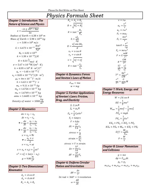
Please Do Not Write on This Sheet
Physics Formula Sheet Chapter 1: Introduction: The Nature of Science and Physics
𝑥=−𝑏±√𝑏2−4𝑎𝑐
2𝑎
𝑅𝑎𝑑𝑖𝑢𝑠 𝑜𝑓 𝐸𝑎𝑟𝑡ℎ=6.38×10⁶ 𝑚
𝑀𝑎𝑠𝑠 𝑜𝑓 𝐸𝑎𝑟𝑡ℎ=5.98×1024 𝑘𝑔
𝑐=3.00×10⁸ 𝑚/𝑠
𝐺=6.673×10⁻¹¹𝑁𝑚2
𝑘𝑔2
𝑁
𝐴=6.02×10²³
𝑘=1.38×10⁻²³𝐽/𝐾
𝑅=8.31𝐽𝑚𝑜𝑙⋅𝐾⁄
𝜎=5.67×10⁻⁸𝑊/(𝑚2⋅𝐾)
𝑘=8.99×10⁹ 𝑁⋅𝑚2/𝐶2
𝑞
𝑒=−1.60×10⁻¹⁹ 𝐶
𝜖
0=8.85×10⁻¹²𝐶2/(𝑁⋅𝑚2)
𝜇
0=4π×10−7 𝑇⋅𝑚/𝐴
ℎ=6.63×10⁻³⁴ 𝐽⋅𝑠
𝑚
𝑒=9.11×10⁻³¹ 𝑘𝑔
𝑚
𝑝=1.6726×10⁻²⁷ 𝑘𝑔
𝑚
𝑛=1.6749×10⁻²⁷ 𝑘𝑔
𝑎𝑚𝑢=1.6605×10⁻²⁷ 𝑘𝑔
𝐷𝑒𝑛𝑠𝑖𝑡𝑦 𝑜𝑓 𝑤𝑎𝑡𝑒𝑟=1000𝑘𝑔
𝑚3
Chapter 2: Kinematics
𝛥𝑥=𝑥
𝑓−𝑥
0
𝛥𝑡=𝑡
𝑓−𝑡
0
𝑣=𝛥𝑥
𝛥𝑡=𝑥
𝑓−𝑥
0
𝑡
𝑓−𝑡
0
𝑎=𝛥𝑣
𝛥𝑡=𝑣
𝑓−𝑣
0
𝑡
𝑓−𝑡
0
𝑥=𝑥
0+𝑣𝑡
𝑣=𝑣
0+𝑣
2
𝑣=𝑣
0+𝑎𝑡
𝑥=𝑥
0+𝑣
0𝑡+1
2𝑎𝑡2
𝑣2=𝑣
02+2𝑎(𝑥−𝑥
0)
𝑔=9.80𝑚
𝑠2
Chapter 3: Two-Dimensional
Kinematics

Computational Electrodynamics: The Finite-Difference Time-Domain Method, 3rd ed. A. Taflove, S. C. Hagness CHAPTER 5 – SOLUTIONS TO SELECTED PROBLEMS
41 Problem 5.1 In this illustrative solution, the electric-field hard source condition of (5.1) is implemented at the far-left grid boundary. The source time function has an amplitude of 1.0 V/m and a frequency of 10 GHz. The reflecting barrier (PEC) is implemented at the far-right grid boundary. The computational domain represents a physical length of 15 cm. Matlab code: %*********************************************************************** % 1D FINITE-DIFFERENCE TIME-DOMAIN SOLUTION: PLANE WAVE PROPAGATION %*********************************************************************** % % Program author: % Prof. Susan C. Hagness % Department of Electrical and Computer Engineering % University of Wisconsin-Madison % 1415 Engineering Drive % Madison, WI 53706-1691 % hagness@ % %*********************************************************************** clear; %..........Material Parameters............ cc=2.99792458e8; %speed of light in free space muz=4.0*pi*1.0e-7; %permeability of free space epsz=1.0/(cc*cc*muz); %permittivity of free space eps=[1.0]; %relative permittivity sig=[0.0]; %electric conductivity mur=[1.0]; %relative permeability sim=[0.0]; %magnetic loss media=length(eps); %..........Space, Time, and Source Parameters... S=1.0; freq=10e9; %frequency of sinusoidal excitation = 10 GHz E0=1.0; %amplitude of sinusoidal excitation = 1.0 V/m lambda=cc/freq; length=0.15; %physical length of grid (in units of m) dx=lambda/20; %grid resolution of 20 cells per wavelength dt=S*dx/cc; ie=round(length/dx)+1; %number of Ez samples in grid ih=ie-1; %number of Hy samples in grid nmax=3*round(ie*S); source(1:nmax)=E0*sin(2*pi*freq*(1:nmax)*dt); %..........Initial Conditions........... ez(1:ie)=0.0; hy(1:ih)=0.0; Computational Electrodynamics: The Finite-Difference Time-Domain Method, 3rd ed. A. Taflove, S. C. Hagness CHAPTER 5 – SOLUTIONS TO SELECTED PROBLEMS
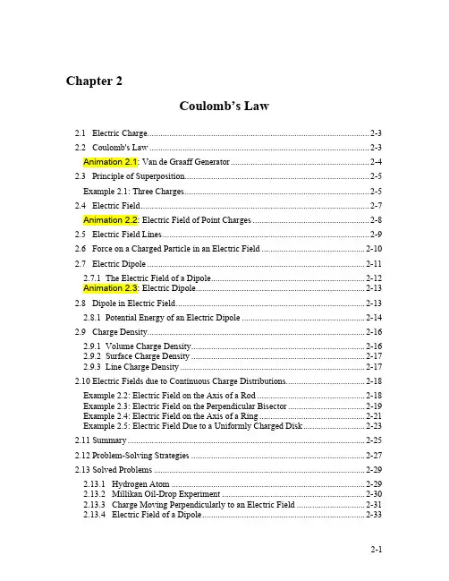
Chapter 2
Coulomb’s Law
2.1 Electric Charge.....................................................................................................2-3
2.2 Coulomb's Law....................................................................................................2-3
Animation 2.1: Van de Graaff Generator...............................................................2-4
2.3 Principle of Superposition....................................................................................2-5
Example 2.1: Three Charges....................................................................................2-5
2.4 Electric Field........................................................................................................2-7
Animation 2.2: Electric Field of Point Charges.....................................................2-8