ECCV2014 best paper

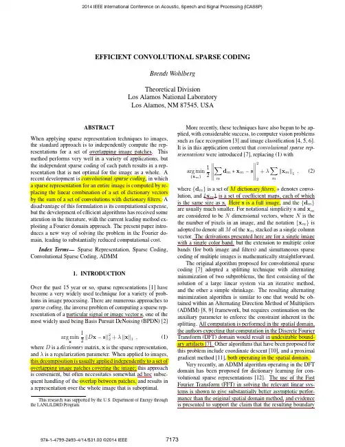
EFFICIENT CONVOLUTIONAL SPARSE CODINGBrendt WohlbergTheoretical DivisionLos Alamos National LaboratoryLos Alamos,NM87545,USAABSTRACTWhen applying sparse representation techniques to images,the standard approach is to independently compute the rep-resentations for a set of image patches.Thismethod performs very well in a variety of applications,butthe independent sparse coding of each patch results in a rep-resentation that is not optimal for the image as a whole.Arecent development is convolutional sparse coding,in whicha sparse representation for an entire image is computed by re-placing the linear combination of a set of dictionary vectorsby the sum of a set of convolutions with dictionaryfilters.Adisadvantage of this formulation is its computational expense,but the development of efficient algorithms has received someattention in the literature,with the current leading method ex-ploiting a Fourier domain approach.The present paper intro-duces a new way of solving the problem in the Fourier do-main,leading to substantially reduced computational cost.Index Terms—Sparse Representation,Sparse Coding,Convolutional Sparse Coding,ADMM1.INTRODUCTIONOver the past15year or so,sparse representations[1]havebecome a very widely used technique for a variety of prob-lems in image processing.There are numerous approaches tosparse coding,the inverse problem of computing a sparse rep-resentation of a signal or image vector s,one of themost widely used being Basis Pursuit DeNoising(BPDN)[2]arg minx 12D x−s 22+λ x 1,(1)where D is a dictionary matrix,x is the sparse representation, andλis a regularization parameter.When applied to images, decomposition is usually applied independently to a set of overlapping image patches covering the image;this approach is convenient,but often necessitates somewhat ad hoc subse-quent handling of the overlap between patches,and results in a representation over the whole image that is suboptimal.This research was supported by the U.S.Department of Energy through the LANL/LDRD Program.More recently,these techniques have also begun to be ap-plied,with considerable success,to computer vision problems such as face recognition[3]and image classification[4,5,6]. It is in this application context that convolutional sparse rep-resentations were introduced[7],replacing(1)with arg min{x m}12md m∗x m−s22+λmx m 1,(2)where{d m}is a set of M dictionaryfilters,∗denotes convo-lution,and{x m}is a set of coefficient maps,each of which is the same size as s.Here s is a full image,and the{d m} are usually much smaller.For notational simplicity s and x m are considered to be N dimensional vectors,where N is the the number of pixels in an image,and the notation{x m}is adopted to denote all M of the x m stacked as a single column vector.The derivations presented here are for a single image with a single color band,but the extension to multiple color bands(for both image andfilters)and simultaneous sparse coding of multiple images is mathematically straightforward.The original algorithm proposed for convolutional sparse coding[7]adopted a splitting technique with alternating minimization of two subproblems,thefirst consisting of the solution of a large linear system via an iterative method, and the other a simple shrinkage.The resulting alternating minimization algorithm is similar to one that would be ob-tained within an Alternating Direction Method of Multipliers (ADMM)[8,9]framework,but requires continuation on the auxiliary parameter to enforce the constraint inherent in the splitting.All computation is performed in the spatial domain, the authors expecting that computation in the Discrete Fourier Transform(DFT)domain would result in undesirable bound-ary artifacts[7].Other algorithms that have been proposed for this problem include coordinate descent[10],and a proximal gradient method[11],both operating in the spatial domain.Very recently,an ADMM algorithm operating in the DFT domain has been proposed for dictionary learning for con-volutional sparse representations[12].The use of the Fast Fourier Transform(FFT)in solving the relevant linear sys-tems is shown to give substantially better asymptotic perfor-mance than the original spatial domain method,and evidence is presented to support the claim that the resulting boundary2014 IEEE International Conference on Acoustic, Speech and Signal Processing (ICASSP)effects are not significant.The present paper describes a convolutional sparse coding algorithm that is derived within the ADMM framework and exploits the FFT for computational advantage.It is very sim-ilar to the sparse coding component of the dictionary learning algorithm of[12],but introduces a method for solving the linear systems that dominate the computational cost of the al-gorithm in time that is linear in the number offilters,instead of cubic as in the method of[12].2.ADMM ALGORITHMRewriting(2)in a form suitable for ADMM by introducing auxiliary variables{y m},we havearg min {x m},{y m}12md m∗x m−s22+λmy m 1 such that x m−y m=0∀m,(3)for which the corresponding iterations(see[8,Sec.3]),with dual variables{u m},are{x m}(k+1)=arg min{x m}12md m∗x m−s22+ρ2mx m−y(k)m+u(k)m22(4){y m}(k+1)=arg min{y m}λmy m 1+ρ2mx(k+1)m−y m+u(k)m22(5)u(k+1) m =u(k)m+x(k+1)m−y(k+1)m.(6)Subproblem(5)is solved via shrinkage/soft thresholding asy(k+1) m =Sλ/ρx(k+1)m+u(k)m,(7)whereSγ(u)=sign(u) max(0,|u|−γ),(8) with sign(·)and|·|of a vector considered to be applied element-wise.The computational cost is O(MN).The only computationally expensive step is solving(4), which is of the formarg min {x m}12md m∗x m−s22+ρ2mx m−z m 22.(9)2.1.DFT Domain FormulationAn obvious approach is to attempt to exploit the FFT for ef-ficient implementation of the convolution via the DFT convo-lution theorem.(This does involve some increase in memory requirement since the d m are zero-padded to the size of the x m before application of the FFT.)Define linear operators D m such that D m x m=d m∗x m,and denote the variables D m,x m,s,and z m in the DFT domain byˆD m,ˆx m,ˆs,andˆz m respectively.It is easy to show via the DFT convolution theorem that(9)is equivalent toarg min{ˆx m}12mˆDmˆx m−ˆs22+ρ2mˆx m−ˆz m 22(10)with the{x m}minimizing(9)being given by the inverse DFT of the{ˆx m}minimizing(10).DefiningˆD= ˆDˆD1...,ˆx=⎛⎜⎝ˆx0ˆx1...⎞⎟⎠,ˆz=⎛⎜⎝ˆz0ˆz1...⎞⎟⎠,(11) this problem can be expressed asarg minˆx12ˆDˆx−ˆs22+ρ2ˆx−ˆz 22,(12) the solution being given by(ˆD HˆD+ρI)ˆx=ˆD Hˆs+ρˆz.(13) 2.2.Independent Linear SystemsMatrixˆD has a block structure consisting of M concatenated N×N diagonal matrices,where M is the number offilters and N is the number of samples in s.ˆD HˆD is an MN×MN matrix,but due to the diagonal block(not block diagonal) structure ofˆD,a row ofˆD H with its non-zero element at col-umn n will only have a non-zero product with a column ofˆD with its non-zero element at row n.As a result,there is no interaction between elements ofˆD corresponding to differ-ent frequencies,so that(as pointed out in[12])one need only solve N independent M×M linear systems to solve(13). Bristow et al.[12]do not specify how they solve these linear systems(and their software implementation was not available for inspection),but since they rate the computational cost of solving them as O(M3),it is reasonable to conclude that they apply a direct method such as Gaussian elimination.This can be very effective[8,Sec. 4.2.3]when it is possible to pre-compute and store a Cholesky or similar decomposition of the linear system(s),but in this case it is not practical unless M is very small,having an O(M2N)memory requirement for storage of these decomposition.Nevertheless,this remains a reasonable approach,the only obvious alternative being an iterative method such as conjugate gradient(CG).A more careful analysis of the unique structure of this problem,however,reveals that there is an alternative,and vastly more effective,solution.First,define the m th block of the right hand side of(13)asˆr m=ˆD H mˆs+ρˆz m,(14)so that⎛⎜⎝ˆr 0ˆr 1...⎞⎟⎠=ˆDH ˆs +ρˆz .(15)Now,denoting the n th element of a vector x by x (n )to avoid confusion between indexing of the vectors themselves and se-lection of elements of these vectors,definev n =⎛⎜⎝ˆx 0(n )ˆx 1(n )...⎞⎟⎠b n =⎛⎜⎝ˆr 0(n )ˆr 1(n )...⎞⎟⎠,(16)and define a n as the column vector containing all of the non-zero entries from column n of ˆDH ,i.e.writing ˆD =⎛⎜⎜⎜⎝ˆd 0,00...ˆd 1,00...0ˆd 0,10...0ˆd 1,10...00ˆd 0,2...00ˆd 1,2...........................⎞⎟⎟⎟⎠(17)thena n =⎛⎜⎝ˆd ∗0,nˆd ∗1,n ...⎞⎟⎠,(18)where ∗denotes complex conjugation.The linear system to solve corresponding to element n of the {x m }is (a n a H n +ρI )v n =b n .(19)The critical observation is that the matrix on the left handside of this system consists of a rank-one matrix plus a scaled identity.Applying the Sherman-Morrison formula(A +uv H )−1=A −1−A −1uv H A −11+u H A −1v (20)gives(ρI +aa H )−1=ρ−1 I −aaHρ+a H a,(21)so that the solution to (19)isv n =ρ−1b n −a H n b nρ+a H n a na n.(22)The only vector operations here are inner products,element-wise addition,and scalar multiplication,so that this method is O (M )instead of O (M 3)as in [12].The cost of solving N of these systems is O (MN ),and the cost of the FFTs is O (MN log N ).Here it is the cost of the FFTs that dominates,whereas in [12]the cost of solving the DFT domain linear systems dominates the cost of the FFTs.This approach can be implemented in an interpreted lan-guage such as Matlab in a form that avoids explicit iteration over the N frequency indices by passing data for all N in-dices as a single array to the relevant linear-algebraic routines (commonly referred to as vectorization in Matlab terminol-ogy).Some additional computation time improvement is pos-sible,at the cost of additional memory requirements,by pre-computing a H n /(ρ+a Hn a n )in (22).2.3.Algorithm SummaryThe proposed algorithm is summarized in Alg.1.stop-ping criteria are those discussed in [8,Sec.3.3],together withan upper bound on the number of iterations.The options for the ρupdate are (i)fixed ρ(i.e.no update),(ii)the adaptive update strategy described in [8,Sec. 3.4.1],and the multi-plicative increase scheme advocated in [12].Input :image s ,filter dictionary {d m },parameters λ,ρPrecompute:FFTs of {d m }→{ˆDm },FFT of s →ˆs Initialize:{y m }={u m }=0while stopping criteria not met doCompute FFTs of {y m }→{ˆym },{u m }→{ˆu m }Compute {ˆxm }using the method in Sec.2.2Compute inverse FFTs of {ˆxm }→{x m }{y m }=S λ/ρ({x m }+{u m }){u m }={u m }+{x m }−{y m }Update ρif appropriate endOutput :Coefficient maps {x m }Algorithm 1:Summary of proposed ADMM algorithm The computational cost of the algorithm components is O (MN log N )for the FFTs,order O (MN )for the proposed linear solver,and O (MN )for both the shrinkage and dual variable update,so that the cost of the entire algorithm is O (MN log N ),dominated by the cost of FFTs.In contrast,the cost of the algorithm proposed in [12]is O (M 3N )(there is also an O (MN log N )cost for FFTs,but it is dominated by the O (M 3N )cost of the linear solver),and the cost of the original spatial-domain algorithm [7]is O (M 2N 2L ),where L is the dimensionality of the filters.3.DICTIONARY LEARNINGThe extension of (2)to learning a dictionary from training data involves replacing the minimization with respect to x m with minimization with respect to both x m and d m .The op-timization is invariably performed via alternating minimiza-tion between the two variables,the most common approach consisting of a sparse coding step followed by a dictionary update [13].The commutativity of convolution suggests that the DFT domain solution of Sec.2.1can be directly applied in minimizing with respect to d m instead of x m ,but this is not possible since the d m are of constrained size,and must be zero-padded to the size of the x m prior to a DFT domain im-plementation of the convolution.If the size constraint is im-plemented in an ADMM framework [14],however,the prob-lem is decomposed into a computationally cheap subproblem corresponding to a projection onto to constraint set,and an-other subproblem that can be efficiently solved by extending the method in Sec.2.1.This iterative algorithm for the dictio-nary update can alternate with a sparse coding stage to form amore traditional dictionary learning method [15],or the sub-problems of the sparse coding and dictionary update algo-rithms can be combined into a single ADMM algorithm [12].4.RESULTScomparison of execution times for the algorithm (λ=0.05)with different methods of solving the linear system,for a set of overcomplete 8×8DCT dictionaries and the 512×512greyscale Lena image,is presented in Fig.1.It is worth em-phasizing that this is a large image by the standards of prior publications on convolutional sparse coding;the test images in [12],for example,are 50×50and 128×128pixels in size.The Gaussian elimination solution is computed using a Cholesky decomposition (since it is,in general,impossible to cache this decomposition,it is necessary to recompute it at every solution),as implemented by the Matlab mldivide function,and is applied by iterating over all frequencies in the apparent absence of any practical alternative.The conjugate gradient solution is computed using two different relative error tolerances.A significant part of the computational advantage here of CG over the direct method is that it is applied simultaneously over all frequencies.The two curves for the proposed solver based on the Sherman-Morrison formula illustrate the significant gain from an implementation that simultaneously solves over all frequencies and that the relative advantage of doing so de-creases with increasing M .Dictionary size (M )E x e c u t i o n t i m e (s )512256128641e+051e+041e+031e+021e+01Fig.1.A comparison of execution times for 10steps of the ADMM algorithm for different methods of solving the lin-ear system:Gaussian elimination (GE),Conjugate Gradient with relative error tolerance 10−5(CG 10−5)and 10−3(CG 10−3),and Sherman-Morrison implemented with a loop over frequencies (SM-L)or jointly over all frequencies (SM-V).The performance of the three ρupdate strategies dis-cussed in the previous section was compared by sparse cod-ing a 256×256Lena image using a 9×9×512dictionary (from [16],by the authors of [17])with a fixed value of λ=0.02and a range of initial ρvalues ρ0.The resulting values of the functional in (2)after 100,500,and 1000itera-tions of the proposed algorithm are displayed in Table 1.The adaptive update strategy uses the default parameters of [8,Sec. 3.4.1],and the increasing strategy uses a multiplica-tive update by a factor of 1.1with a maximum of 105,as advocated by [12].In summary,a fixed ρcan perform well,but is sensitive to a good choice of parameter.When initialized with a small ρ0,the increasing ρstrategy provides the most rapid decrease in functional value,but thereafter converges very slowly.Over-all,unless rapid computation of an approximate solution is desired,the adaptive ρstrategy appears to provide the best performance,with the least sensitivity to choice of ρ0.This is-sue is complex,however,and further experimentation is nec-essary before drawing any general conclusions that could be considered valid over a broad range of problems.Iter.ρ010−210−1100101102103Fixed ρ10028.2727.8018.1010.099.7611.6050028.0522.2511.118.899.1110.13100027.8017.009.648.828.969.71Adaptive ρ10021.6216.9714.5610.7111.1411.4150010.8110.239.819.019.189.0910009.449.219.068.838.878.84Increasing ρ10014.789.829.509.9011.5115.155009.559.459.469.8911.4714.5110009.539.449.459.8811.4113.97Table parison of functional value convergence for thesame problem with three different ρupdate strategies.5.CONCLUSIONA computationally efficient algorithm is proposed for solving the convolutional sparse coding problem in the Fourier do-main.This algorithm has the same general structure as a pre-viously proposed approach [12],but enables a very significantreduction in computational cost by careful design of a linear solver for the most critical component of the iterative algo-rithm.The theoretical computational cost of the algorithm is reduced from O (M 3)to O (MN log N )(where N is the di-mensionality of the data and M is the number of elementsin the dictionary),and is also shown empirically to result in greatly reduced computation time.The significant improve-ment in efficiency of the proposed approach is expected togreatly increase the range of problems that can practically be addressed via convolutional sparse representations.6.REFERENCES[1]A.M.Bruckstein,D.L.Donoho,and M.Elad,“Fromsparse solutions of systems of equations to sparse mod-eling of signals and images,”SIAM Review,vol.51, no.1,pp.34–81,2009.doi:10.1137/060657704[2]S.S.Chen,D.L.Donoho,and M.A.Saunders,“Atomicdecomposition by basis pursuit,”SIAM Journal on Sci-entific Computing,vol.20,no.1,pp.33–61,1998.doi:10.1137/S1064827596304010[3]J.Wright,A.Y.Yang,A.Ganesh,S.S.Sastry,andY.Ma,“Robust face recognition via sparse representa-tion,”IEEE Transactions on Pattern Analysis and Ma-chine Intelligence,vol.31,no.2,pp.210–227,February 2009.doi:10.1109/tpami.2008.79[4]Y.Boureau,F.Bach,Y.A.LeCun,and J.Ponce,“Learn-ing mid-level features for recognition,”in Proceedings of the IEEE Conference on Computer Vision and Pat-tern Recognition(CVPR),June2010,pp.2559–2566.doi:10.1109/cvpr.2010.5539963[5]J.Yang,K.Yu,and T.S.Huang,“Supervisedtranslation-invariant sparse coding,”Proceedings of the IEEE Conference on Computer Vision and Pat-tern Recognition(CVPR),pp.3517–3524,2010.doi:10.1109/cvpr.2010.5539958[6]J.Mairal,F.Bach,and J.Ponce,“Task-driven dictionarylearning,”IEEE Transactions on Pattern Analysis and Machine Intelligence,vol.34,no.4,pp.791–804,April 2012.doi:10.1109/tpami.2011.156[7]M.D.Zeiler,D.Krishnan,G.W.Taylor,and R.Fer-gus,“Deconvolutional networks,”in Proceedings of the IEEE Conference on Computer Vision and Pat-tern Recognition(CVPR),June2010,pp.2528–2535.doi:10.1109/cvpr.2010.5539957[8]S.Boyd,N.Parikh,E.Chu,B.Peleato,and J.Eckstein,“Distributed optimization and statistical learning via the alternating direction method of multipliers,”Founda-tions and Trends in Machine Learning,vol.3,no.1,pp.1–122,2010.doi:10.1561/2200000016[9]J.Eckstein,“Augmented Lagrangian and alternatingdirection methods for convex optimization:A tutorial and some illustrative computational results,”Rutgers Center for Operations Research,Rutgers University, Rutcor Research Report RRR32-2012,December 2012.[Online].Available:/pub/ rrr/reports2012/322012.pdf[10]K.Kavukcuoglu,P.Sermanet,Y.Boureau,K.Gregor,M.Mathieu,and Y.A.LeCun,“Learning convolutionalfeature hierachies for visual recognition,”in Advances in Neural Information Processing Systems(NIPS2010), 2010.[11]R.Chalasani,J.C.Principe,and N.Ramakrishnan,“A fast proximal method for convolutional sparse cod-ing,”in Proceedings of the International Joint Confer-ence on Neural Networks(IJCNN),Aug.2013,pp.1–5.doi:10.1109/IJCNN.2013.6706854[12]H.Bristow, A.Eriksson,and S.Lucey,“Fast con-volutional sparse coding,”in Proceedings of the IEEE Conference on Computer Vision and Pat-tern Recognition(CVPR),Jun.2013,pp.391–398.doi:10.1109/CVPR.2013.57[13]B.Mailh´e and M.D.Plumbley,“Dictionary learningwith large step gradient descent for sparse representa-tions,”in Latent Variable Analysis and Signal Sepa-ration,ser.Lecture Notes in Computer Science,F.J.Theis,A.Cichocki,A.Yeredor,and M.Zibulevsky,Eds.Springer Berlin Heidelberg,2012,vol.7191,pp.231–238.doi:10.1007/978-3-642-28551-629[14]M.V.Afonso,J.M.Bioucas-Dias,and M. A.T.Figueiredo,“An Augmented Lagrangian approach to the constrained optimization formulation of imaging inverse problems,”IEEE Transactions on Image Pro-cessing,vol.20,no.3,pp.681–695,March2011.doi:10.1109/tip.2010.2076294[15]K.Engan,S.O.Aase,and J.H.Husøy,“Method ofoptimal directions for frame design,”in Proceedings of the IEEE International Conference on Acoustics, Speech,and Signal Processing(ICASSP),vol.5,1999, pp.2443–2446.doi:10.1109/icassp.1999.760624 [16]J.Mairal,Software available from http://lear.inrialpes.fr/people/mairal/denoise ICCV09.tar.gz.[17]J.Mairal,F.Bach,J.Ponce,G.Sapiro,and A.Zis-serman,“Non-local sparse models for image restora-tion,”in Proceedings of the IEEE International Con-ference on Computer Vision(CVPR),2009,pp.2272–2279.doi:10.1109/iccv.2009.5459452。

2014 International Conference on Computer Science and Electronic Technology (ICCSET 2014)Fast Image Retrieval Based on Two-dimensional EmbeddingKui Zhao1,a, Shihan Wang1,b, Wei Wang1,c1Zhejiang Provincial Key Laboratory of Service Robot, College of Computer Science, ZhejiangUniversity, Hangzhou 310027, Chinaa***************.cn,b*********************,c*********************.cn Keywords: Image Retrieve; Two-dimensional Embedding; Nearest Neighbor SearchAbstract. Recent years see an explosive growth of digital images and we need efficient technologies to index and retrieve them. The content-based retrieval method is a hot topic in recent research, in which we index the features of image and then retrieve the images through nearest neighbor searching. The features of an image dwell in high dimensional space, which poses particular challenge for nearest neighbor search. The curse of dimensionality raises severe difficulty in traditional methods. In this paper, we proposed a novel method for nearest neighbor search in high dimensional space based on two-dimensional embedding. First, we filter out the non-nearest neighbors using low dimensional information via data embedding, and then efficient nearest neighbor search can be performed in a much smaller candidate set to achieve fast image retrieval. The experimental results on the dataset CIFAR validate the effectiveness and efficiency of our method.IntroductionThe rapid development of the Internet triggers an explosion of the available information, especially complex information such as images and videos. Efficiently indexing and retrieving huge volumes of images become a hot topic both in academia and industry.Traditional methods for indexing and retrieving of images are dependent on manual text marking. Once we have textual information, such as titles or keywords, the problem is transformed into textual retrieval problem. There are a lot of well-developed methods to do textual retrieval. However, because the textual information marked by hand is usually not sufficient enough to represent the images, the performance of this kind of methods is not very satisfying. What’s more, the manual text marking on large data set is very expensive. Another direction is indexing and retrieving the images based on the content of the images [1]. In these methods, when retrieving an image we return the k nearest neighbors, which are k nearest images in the content space of these images. The nearest neighbor search (NNS) algorithm is the most important part for this kind of methods, which almost decides the overall speed and precision of the content-based retrieval.In this paper, we proposed a fast method for image retrieval based on two-dimensional embedding NNS. We filter out the non-nearest neighbors, which are in high dimensional space, only using low dimensional information through data embedding. Then we can search the nearest neighbor in a much smaller candidate set in which the data points are in high dimensional space. This strategy makes it very fast to find the nearest neighbor and our experimental results on the dataset CIFAR validate the effectiveness and efficiency of our method compared with other methods.Related WorkThe KD-Tree proposed by Smeulders, A. W. etc. is a very famous algorithm based on space division for NNS [2]. They divide the data space equally according to variance recursively and query a point using the relation between query point and division plane. Y Beis, J. S. and Lowe, D. G [3] presented an approximate nearest searching by introducing the best bin first strategy. The vantage point tree [4] and multi vantage point tree [5] are both based on triangle inequality for space division. The performance of those methods is very good in low dimensional space, but the performance declines significantly in high dimensional space.In order to achieve better performance in high dimensional space, many methods have been proposed. The locality-sensitive hashing [6] reduces dimension according to probability information. The hierarchical K-means tree method [7] uses clustering to construct a tree and choose searching path according to the distances between the query point and center of clusters. The Cover-Tree [8] also constructs a tree data structure for NNS. However, the performance of these methods is also not good enough for high dimensional data.Two-dimensional Embedding for Nearest Neighbor SearchingThe data embedding is used widely in processing high dimensional data. In this paper, we embed the high dimensional data into a low dimensional space inspired by the lower and upper bound of Euclidean distance [9]. For point x and y in Euclidean space,222dist(,)[()()]d µµs s ≥×−+−x y x y x y , (1)222dist(,)[()()]d µµs s ≤×−++x y x y x y . (2) Where d is the dimension of x , µx and s x are the mean and variance value of x over its entire dimension respectively. We project the high dimensional data point x to two two-dimensional points (,)µs x x and (,)µs −x x , represented by x + and x -. So the lower bound of squared Euclidean distance between x and y is 2dist(x ,y )d ++× and the upper bound is 2dist(x ,y )d +−×.Then we can design a fast method for nearest neighbor search using vantage point tree (VP-Tree) and two-dimensional embedding mentioned above. The algorithm is shown in Algorithm 1. Algorithm 1 NNS Based on Two-dimensional EmbeddingInput : Searching data point set {x }, dimenson d of x and query point q ;Output : Nearest neighbor point for query point q ;Initialization : candidate = NULL, min_dist = ∞Caculate the projection set {x +} and {x -} for {x };Construct VP-Tree for {x +} and {x -}, denoted by VPT +, VPT -;Caculate the projection q + for q ;Find the nearest point to q + in VPT - and denote the distance as U min ;Find the points in VPT + whose distance to q + are less than U min ,and put these points in the set {x }*;for each x i in {x }*if d×dist(x i +, q +)2 ≥ min_dist 2continue;else. if dist(x i , q )2 < min_dist 2. candidate = x i , min_dist 2 = dist(x i , q )2;. end. end. Return candidateAs we can see, after filtering the non-nearest neighbor points, we can search the nearest neighbor point in a much smaller set {x }*. For a special data set, we only need to run step 1-2 of Algorithm 1 one time. When we query point q , we run Algorithme from step 3 to the end.Experimental ResultsIn the experimental evaluation, the data set we have used is CIFAR [10], which contains 50,000 color images. The image in this data set has 32×32 pixel points, each pixel point is represented by three number which ranges in [0, 255], so the dimension of each image is 32×32×3 = 3072. Most of methods for nearest neighbor search cannot work efficiently in such a high dimensional space. Besides, we construct two new data sets from the original one, the size of images in them are 24×24and 16×16 respectively. For each data set, we choose 100 images randomly as query set and the remaining 49,900 images as data set for searching.First, we focus on the filtering rate of our method. The experiments on different data sets will show us the dimension of data affect the filtering rate. The filtering rates of our method on different data sets are shown in Table1.Table1 The filtering rates on different data setsSize of image Filtering rate max Filtering rate max Filtering rate mean Filtering rate variance 16×16 96.8% 24.6% 59.4% 0.04224×24 96.8% 23.3% 58.2% 0.04332×32 95.4% 12.8% 46.8% 0.060As we can see, the filtering rates of query points are quite different. The maximum filtering rates are all above 95%, but the minimum filtering rate and average filtering rate decrease when the dimension increases. What’s more, the filtering rate is more unstable in high dimensional space.In order to indicate the effectiveness of our method, we compare its searching time with Cover-Tree [10], and the baseline is linear scanning. Linear scanning will compare the query point with all points in the searching data set, which is the worst case. The average query time for different method is shown in Table2.Table2 The average time for different methodsSize of image Our Method Cover-Tree Linear Scanning 16×16 0.0996s 0.142s 0.268s24×24 0.0867s 0.282s 0.606s32×32 0.248s 0.416s 1.03s We also normalize the average query time by setting the time of linear scanning to be 1.0. The results are presented in Table3.Table3 The normalized average time of different methodsSize of image Our Method Cover-Tree Linear Scanning 16×16 0.188 0.530 1.024×24 0.186 0.466 1.032×32 0.241 0.404 1.0 As we can see, the efficiency of our method is improved at least 4 times compared with linear scanning and 1.6 times compared with Cover-Tree. What’s more, the efficiency improvement in low dimensional space is even more significant.SummaryWe have proposed a novel method for nearest neighbor search based on two-dimensional embedding. We filter out the non-nearest neighbors using low dimensional information, and then search the nearest neighbor much faster in a smaller candidate set. The experimental results on the dataset CIFAR indicate the effectiveness and efficiency of our method. The method we proposed can be used for fast content-based image retrieval or other high dimensional data retrieval, such as video retrieval.For future work, we consider making our method more stable for different query points through better data embedding algorithm. We also consider designing a more efficient strategy to choose the threshold for filtering out the non-nearest neighbors. This way, we can apply our method in many practical situations and optimize its performance accordingly, as well as making it more robust. All of these works will improve the practicability of our method for searching the nearest neighbor in high dimensional space.AcknowledgementThis work is supported by National Key Technology R&D Program (Grant No. 2012BAI34B01).References[1] Smeulders, A. W., Worring, M., Santini, S., Gupta, A., & Jain, R. (2000). Content-based image retrieval at the end of the early years. Pattern Analysis and Machine Intelligence, IEEE Transactions on, 22(12), 1349-1380.[2] Bentley, J. L. (1975). Multidimensional binary search trees used for associative searching. Communications of the ACM, 18(9), 509-517.[3] Y Beis, J. S., & Lowe, D. G. (1997, June). Shape indexing using approximate nearest-neighbour search in high-dimensional spaces. In Computer Vision and Pattern Recognition, 1997. Proceedings., 1997 IEEE Computer Society Conference on (pp. 1000-1006). IEEE.[4] Yianilos, P. N. (1993, January). Data structures and algorithms for nearest neighbor search in general metric spaces. In Proceedings of the fourth annual ACM-SIAM Symposium on Discrete algorithms (pp. 311-321). Society for Industrial and Applied Mathematics.[5] Bozkaya, T., & Ozsoyoglu, M. (1997, June). Distance-based indexing for high-dimensional metric spaces. In ACM SIGMOD Record (Vol. 26, No. 2, pp. 357-368). ACM.[6] Datar, M., Immorlica, N., Indyk, P., & Mirrokni, V. S. (2004, June). Locality-sensitive hashing scheme based on p-stable distributions. In Proceedings of the twentieth annual symposium on Computational geometry (pp. 253-262). ACM.[7] Fukunaga, K., & Narendra, P. M. (1975). A branch and bound algorithm for computing k-nearest neighbors. Computers, IEEE Transactions on, 100(7), 750-753.[8] Beygelzimer, A., Kakade, S., & Langford, J. (2006, June). Cover trees for nearest neighbor. In Proceedings of the 23rd international conference on Machine learning (pp. 97-104). ACM.[9] Hwang, Y., & Ahn, H. K. (2011). Convergent bounds on the euclidean distance. In Advances in Neural Information Processing Systems (pp. 388-396).[10] Krizhevsky, A., & Hinton, G. (2009). Learning multiple layers of features from tiny images. Computer Science Department, University of Toronto, Tech. Rep.。