MATLAB课后上机实验

Matlab 上机实验一、二1．安装Matlab 软件。

2．验证所学内容和教材上的例子。

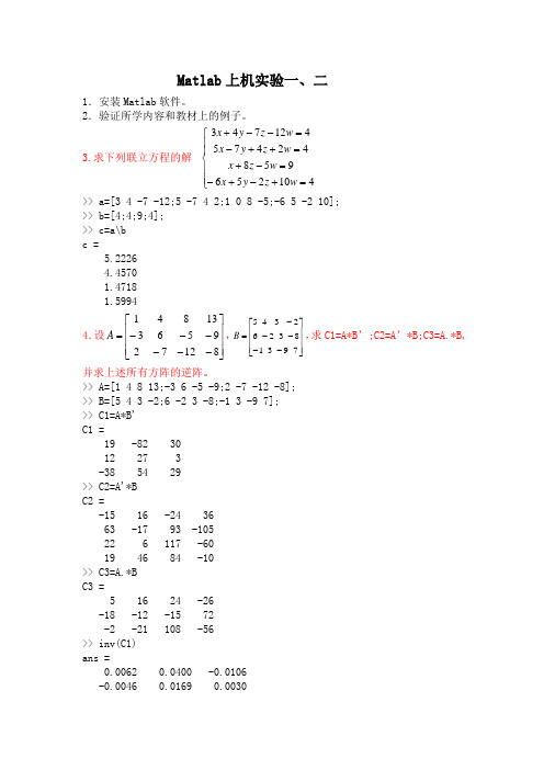
3.求下列联立方程的解⎪⎩⎪⎪⎨⎧=+-+-=-+=++-=--+41025695842475412743w z y x w z x w z y x w z y x >> a=[3 4 -7 -12;5 -7 4 2;1 0 8 -5;-6 5 -2 10];>> b=[4;4;9;4];>> c=a\bc =5.22264.45701.47181.59944．设⎥⎥⎥⎦⎤⎢⎢⎢⎣⎡------=81272956313841A ，⎥⎥⎥⎦⎤⎢⎢⎢⎣⎡-----=793183262345B ，求C1=A*B’;C2=A’*B;C3=A.*B,并求上述所有方阵的逆阵。

>> A=[1 4 8 13;-3 6 -5 -9;2 -7 -12 -8];>> B=[5 4 3 -2;6 -2 3 -8;-1 3 -9 7];>> C1=A*B'C1 =19 -82 3012 27 3-38 54 29>> C2=A'*BC2 =-15 16 -24 3663 -17 93 -10522 6 117 -6019 46 84 -10>> C3=A.*BC3 =5 16 24 -26-18 -12 -15 72-2 -21 108 -56>> inv(C1)ans =0.0062 0.0400 -0.0106-0.0046 0.0169 0.00300.0168 0.0209 0.0150>> inv(C2)Warning: Matrix is close to singular or badly scaled.Results may be inaccurate. RCOND = 8.997019e-019.ans =1.0e+015 *-0.9553 -0.2391 -0.1997 0.27000.9667 0.2420 0.2021 -0.2732-0.4473 -0.1120 -0.0935 0.1264-1.1259 -0.2818 -0.2353 0.31825．设 ⎥⎦⎤⎢⎣⎡++=)1(sin 35.0cos 2x x x y ，把x=0~2π间分为101点，画出以x 为横坐标，y 为纵坐标的曲线。

《MATLAB程序设计与应用》实验指导书实验一 matlab 集成环境使用与运算基础1，先求下列表达式的值，然后显示matlab 工作空间的使用情况并保存全部变量。

（1）0122sin851z e =+程序：.>> z1=2*sin(85*pi/180)/(1+exp(2)) 结果： z1 =0.2375（2）22121(0.4552i z In x x +⎡⎤=+=⎢⎥-⎣⎦其中 程序：>> x=[2,1+2*i;-0.45,5];>> z2=0.5*log(x+sqrt(1+x*x)) 结果： z2 =0.7114 - 0.0253i 0.8968 + 0.3658i 0.2139 + 0.9343i 1.1541 - 0.0044i（3）0.3,9.2,8.2,...,8.2,9.2,0.3,23.0)3.0sin(23.03.03---=+++-=-a aIn a e e z a a 提示：利用冒号表达式生成a 向量，求各点函数值时用点乘运算。

程序：>> a=-3.0:0.1:30;>> z3=(exp(0.3*a)-exp(-0.3*a))/2.*sin((a+0.3)*pi/180)+log((0.3+a)/2) 结果： z3 =1.0e+003 *Columns 1 through 40.0003 + 0.0031i 0.0003 + 0.0031i 0.0003 + 0.0031i 0.0002 + 0.0031iColumns 5 through 80.0002 + 0.0031i 0.0001 + 0.0031i 0.0001 + 0.0031i 0.0000 + 0.0031i Columns 9 through 12-0.0000 + 0.0031i -0.0001 + 0.0031i -0.0001 + 0.0031i -0.0002 + 0.0031i Columns 13 through 16-0.0003 + 0.0031i -0.0003 + 0.0031i -0.0004 + 0.0031i -0.0005 + 0.0031i Columns 17 through 20-0.0006 + 0.0031i -0.0007 + 0.0031i -0.0008 + 0.0031i -0.0009 + 0.0031i Columns 21 through 24-0.0010 + 0.0031i -0.0012 + 0.0031i -0.0014 + 0.0031i -0.0016 + 0.0031i Columns 25 through 28-0.0019 + 0.0031i -0.0023 + 0.0031i -0.0030 + 0.0031i -0.0370 Columns 29 through 32-0.0030 -0.0023 -0.0019 -0.0016 Columns 33 through 36-0.0014 -0.0012 -0.0010 -0.0009 Columns 37 through 40-0.0008 -0.0007 -0.0006 -0.0005 Columns 41 through 44-0.0004 -0.0003 -0.0003 -0.0002 Columns 45 through 48-0.0001 -0.0001 -0.0000 0.0000 Columns 49 through 520.0001 0.0001 0.0002 0.0002 Columns 53 through 560.0003 0.0003 0.0003 0.0004 Columns 57 through 600.0004 0.0005 0.0005 0.0005 Columns 61 through 640.0006 0.0006 0.0006 0.0007 Columns 65 through 680.0007 0.0007 0.0008 0.0008 Columns 69 through 720.0008 0.0008 0.0009 0.0009 Columns 73 through 760.0009 0.0010 0.0010 0.0010 Columns 77 through 800.0011 0.0011 0.0011 0.0011 Columns 81 through 840.0012 0.0012 0.0012 0.0013 Columns 85 through 880.0013 0.0013 0.0013 0.0014 Columns 89 through 920.0014 0.0014 0.0015 0.0015 Columns 93 through 960.0015 0.0016 0.0016 0.0016 Columns 97 through 1000.0017 0.0017 0.0017 0.0018 Columns 101 through 1040.0018 0.0018 0.0019 0.0019 Columns 105 through 1080.0020 0.0020 0.0020 0.0021 Columns 109 through 1120.0021 0.0022 0.0022 0.0023 Columns 113 through 1160.0023 0.0024 0.0024 0.0025 Columns 117 through 1200.0025 0.0026 0.0026 0.0027 Columns 121 through 1240.0027 0.0028 0.0029 0.0029 Columns 125 through 1280.0030 0.0031 0.0031 0.0032 Columns 129 through 1320.0033 0.0034 0.0034 0.0035 Columns 133 through 1360.0036 0.0037 0.0038 0.0039 Columns 137 through 1400.0040 0.0041 0.0042 0.0043 Columns 141 through 1440.0044 0.0045 0.0046 0.0047 Columns 145 through 1480.0049 0.0050 0.0051 0.0053 Columns 149 through 1520.0054 0.0056 0.0057 0.0059 Columns 153 through 1560.0060 0.0062 0.0064 0.0066 Columns 157 through 1600.0068 0.0069 0.0071 0.0074 Columns 161 through 1640.0076 0.0078 0.0080 0.0083 Columns 165 through 1680.0085 0.0088 0.0090 0.0093 Columns 169 through 1720.0096 0.0099 0.0102 0.0105 Columns 173 through 1760.0108 0.0112 0.0115 0.0119 Columns 177 through 1800.0123 0.0127 0.0131 0.0135 Columns 181 through 1840.0139 0.0144 0.0148 0.0153 Columns 185 through 1880.0158 0.0163 0.0168 0.0174 Columns 189 through 1920.0180 0.0185 0.0191 0.0198 Columns 193 through 1960.0204 0.0211 0.0218 0.0225 Columns 197 through 2000.0233 0.0241 0.0249 0.0257 Columns 201 through 2040.0265 0.0274 0.0284 0.0293 Columns 205 through 2080.0303 0.0313 0.0324 0.0335 Columns 209 through 2120.0346 0.0358 0.0370 0.0382 Columns 213 through 2160.0395 0.0409 0.0423 0.0437 Columns 217 through 2200.0452 0.0467 0.0483 0.0500 Columns 221 through 2240.0517 0.0534 0.0552 0.0571 Columns 225 through 2280.0591 0.0611 0.0632 0.0654 Columns 229 through 2320.0676 0.0699 0.0723 0.0748 Columns 233 through 2360.0773 0.0800 0.0827 0.0856 Columns 237 through 2400.0885 0.0915 0.0947 0.0979 Columns 241 through 2440.1013 0.1047 0.1083 0.1121 Columns 245 through 2480.1159 0.1199 0.1240 0.1282 Columns 249 through 2520.1326 0.1372 0.1419 0.1467 Columns 253 through 2560.1518 0.1570 0.1624 0.1679 Columns 257 through 2600.1737 0.1796 0.1858 0.1921 Columns 261 through 2640.1987 0.2055 0.2125 0.2198 Columns 265 through 2680.2273 0.2351 0.2431 0.2514 Columns 269 through 2720.2600 0.2689 0.2781 0.2876 Columns 273 through 2760.2974 0.3076 0.3180 0.3289 Columns 277 through 2800.3401 0.3517 0.3637 0.3761 Columns 281 through 2840.3889 0.4021 0.4158 0.4299 Columns 285 through 2880.4446 0.4597 0.4753 0.4915 Columns 289 through 2920.5082 0.5254 0.5433 0.5617 Columns 293 through 2960.5807 0.6004 0.6208 0.6418 Columns 297 through 3000.6636 0.6861 0.7093 0.7333 Columns 301 through 3040.7581 0.7838 0.8103 0.8377 Columns 305 through 3080.8660 0.8952 0.9254 0.9567 Columns 309 through 3120.9890 1.0223 1.0568 1.0924 Columns 313 through 3161.1292 1.1673 1.2066 1.2472Columns 317 through 3201.2892 1.3326 1.3774 1.4237Columns 321 through 3241.4715 1.5210 1.5721 1.6249Columns 325 through 3281.6794 1.7357 1.7940 1.8541Columns 329 through 3311.9163 1.98052.0468（4）⎪⎩⎪⎨⎧=<≤<≤<≤+--=5.2:5.0:0,322110,121,2224t t t t t t t t z 其中提示：用逻辑表达式求分段函数值。

MATLAB上机实验一一、实验目的初步熟悉MATLAB 工作环境，熟悉命令窗口，学会使用帮助窗口查找帮助信息。

命令窗口二、实验内容(1) 熟悉MATLAB 平台的工作环境。

(2) 熟悉MATLAB 的5 个工作窗口。

(3) MATLAB 的优先搜索顺序。

三、实验步骤1. 熟悉MATLAB 的5 个基本窗口①Command Window (命令窗口)②Workspace (工作空间窗口)—③Command History (命令历史记录窗口)④Current Directory (当前目录窗口)⑤Help Window (帮助窗口)(1) 命令窗口(Command Window)。

在命令窗口中依次输入以下命令：>>x=1>> y=[1 2 34 5 67 8 9];>> z1=[1:10],z2=[1:2:5];>> w=linspace(1,10,10);>> t1=ones(3),t2=ones(1,3),t3=ones(3,1)>> t4=ones(3),t4=eye(4)x =1z1 =1 2 3 4 5 6 7 8 9 10 t1 =1 1 11 1 11 1t2 =1 1 1t3 =111t4 =1 1 11 1 11 1 1t4 =1 0 0 00 1 0 00 0 1 00 0 0 1思考题：①变量如何声明，变量名须遵守什么规则、是否区分大小写。

答：（1）变量声明1.局部变量每个函数都有自己的局部变量，这些变量只能在定义它的函数内部使用。

当函数运行时，局部变量保存在函数的工作空间中，一旦函数退出，这些局部变量将不复存在。

脚本（没有输入输出参数，由一系列MATLAB命令组成的M文件）没有单独的工作空间，只能共享调用者的工作空间。

当从命令行调用，脚本变量存在基本工作空间中；当从函数调用，脚本变量存在函数空间中。

2.全局变量在函数或基本工作空间内，用global声明的变量为全局变量。

Matlab上机实验报告实验二读入MATLAB下自带图像pout.tif1）利用亮度变换函数，调整图像亮度。

a)调整范围设定[0 1]，[1 0]，观测显示效果；b)调整范围设定[0.5 0.75]，[1 0]，观测显示效果。

解：a, I=imread('pout.tif');colormap;imshow(I);j=imadjust(I,[0 1],[1 0],1.5);figure;subimage(j);b, >> I=imread('pout.tif');colormap;imshow(I);j=imadjust(I,[0.5 0.75],[1 0],1.5);figure;subimage(j);2）利用对比度拉伸函数，压缩高值灰度（c值自行设定）。

解：I=imread('pout.tif');colormap;subplot(1,2,1);imshow(I);xlabel('a)原始图像');J=double(I);J=100*log(J+1);I=uint8(J);subplot(1,2,2);subimage(J);xlabel('b)非线性变换');3）利用直方图函数，生成并绘制图像直方图。

解：I=imread('pout.tif');subplot(1,2,1);imshow(I);title('原始图像');subplot(1,2,2);imhist(I);4）利用直方图修正函数，生成均衡化后的图像直方图（n值自定设定）。

解：I=imread('pout.tif');figure(1);subplot(1,2,1);imshow(I);xlabel('a)原始图像');J=histeq(I);figure(1);subplot(1,2,2);imshow(J);xlabel('b)直方图均衡');figure(2);imhist(I,100);figure(3);imhist(J,100);实验三1.运行例3、4，显示并分析输出结果，说明逆滤波和维纳滤波的区别。

MATLAB上机指导书上机一 MATLAB编程环境一、上机目的1.熟悉MATLAB的操作环境及基本操作方法2.熟悉MATLAB的通用参数设置3.熟悉 MATLAB的搜索路径及设置方法4.熟悉MATLAB帮助信息的查阅方法二、上机内容和结果1．利用菜单设置MATLAB的Command Window中字体大小，并更改输出格式。

示例：结果：2.在硬盘上创建以自己名字命名的文件夹，将当前路径修改为此文件夹示例：结果：4．完成下列操作：（1）在MATLAB命令窗口输入以下命令>> x=0:pi/10:2*pi;>> y=sin(x);（2）在工作空间选择变量y,在在工作空间窗口选择绘图菜单命令或在工具栏中单击绘图命令按钮，绘制变量y的图形。

结果：5.利用帮助学习save,load命令的用法，将在工作区中变量全部保存在mypath.mat中，清空工作区，重载变量x,y查看变量信息，并把它们保存在mypath.mat中结果：6. 计算y=1.3^3*sin(pi/3)*sqrt(26)(1)结果用format命令按不同格式输出。

（2）观察在进行上述命令计算后历史窗口的变化，用功能将实现回调刚才的计算语句。

（3）回调计算语句，把sin改为sn运行，观察反馈信息，若回调语句在语句后面加“；”，看输出有何不同结果：上机二 Matlab的计算可视化一、上机目的1、理解MATLAB绘图方法2、掌握绘制二维数据曲线图的方法3、掌握用plot函数和fplot函数绘制曲线的方法4、通过练习掌握绘制二维数据曲线图的方法和plot 函数和fplot 函数的使用5、通过练习熟悉三维曲线和曲面图的绘制方法二、上机内容和步骤1．上机内容（1）绘制下列曲线：①33x x y -= ②2221x e y π= ③64222=+y x1.>> x=0:5; >> y=x-x.^3/3; >> plot(y); >>2.>> x=0:0.3:1;>> y=1/(2*pi)*exp(x.^2/2); >> plot(y);3.>> ezplot('x.^2-2*y.^2-64',[-50 50]);（2）通过用plot 和fplot 函数绘制xy 1sin 的曲线，并分析其区别。

实验报告通信工程 1101学号：********* 姓名：李*实验1MATLAB语言上机操作实践一、实验目的：㈠、了解MATLAB语言的主要特点、作用。

㈡、学会MATLAB主界面简单的操作使用方法。

㈢、学习简单的数组赋值、运算、绘图、流程控制编程。

二、实验内容：㈠、简单的数组赋值方法MATLAB中的变量和常量都可以是数组（或矩阵）,且每个元素都可以是复数。

1．在MATLAB指令窗口输入数组A=[1 2 3；4 5 6；7 8 9]，观察输出结果。

然后，键入：A（4,: )=[1 3 5]键入：A (5，2) = 7键入：A（4，3）= abs (A(5，1))键入：A ([2，5]，：) = [ ]键入：A/2键入：A (4，：) = [sqrt(3) (4+5)/6*2 –7]观察以上各输出结果。

将A式中分号改为空格或逗号，情况又如何？请在每式的后面标注其含义。

A=[1 2 3;4 5 6;7 8 9]A =1 2 34 5 67 8 9>> A(4,: )=[1 3 5]A =1 2 34 5 67 8 91 3 5>> A(5, 2)=7A =1 2 34 5 67 8 91 3 50 7 0>> A(4, 3)=abs(A(5, 1))A =1 2 34 5 67 8 91 3 00 7 0>> A([2, 5],: )=[]A =1 2 37 8 91 3 0>> A/2ans =0.5000 1.0000 1.50003.50004.0000 4.50000.5000 1.5000 0>> A(4,: )=[sqrt(3) (4+5)/6*2 -7]A =1.00002.00003.00007.0000 8.0000 9.00001.0000 3.0000 01.7321 3.0000 -7.0000A=[1 2 3,4 5 6,7 8 9]A =1 2 3 4 5 6 7 8 92．在MATLAB指令窗口输入B=[1+2i，3+4i；5+6i ，7+8i], 观察输出结果。

Matlab 上机实验一、 实验目的1、 掌握绘制MATLAB 二维、三维和特殊图形的常用函数；2、 熟悉并掌握图像输入、输出及其常用处理的函数。

二、 实验内容1 绘制函数的网格图和等高线图。

422cos cos y x yex z +-=其中x 的21个值均匀分布在[-5,5]范围，y 的31个值均匀分布在[0,10]，要求将产生的网格图和等高线图画在同一个图形窗口上。

2 绘制三维曲面图，使用纯铜色调色图阵进行着色，并进行插值着色处理。

⎪⎩⎪⎨⎧===s z t s y ts x sin sin cos cos cos230,20ππ≤≤≤≤t s3 已知⎪⎪⎩⎪⎪⎨⎧>++≤+=0),1ln(210,22x x x x e x y π在-5<=x<=5区间绘制函数曲线。

4 已知y1=x2，y2=cos(2x)，y3＝y1*y2，其中x 为取值-2π~2π的等差数列(每次增加0.02π)，完成下列操作：a) 在同一坐标系下用不同的颜色和线型绘制三条曲线，给三条曲线添加图例；b) 以子图形式，分别用条形图、阶梯图、杆图绘制三条曲线，并分别给三个图形添加标题“y1=x^2”，“y2=cos(2x)”和“y3＝y1*y2”。

5 在xy 平面内选择区域[][],,-⨯-8888，绘制函数z =的三种三维曲面图。

6 在[0,4pi]画sin(x),cos(x)(在同一个图象中); 其中cos(x)图象用红色小圆圈画.并在函数图上标注 “y=sin(x)”, “y=cos(x)” ,x 轴,y 轴,标题为“正弦余弦函数图象”.7 分别用线框图和曲面图表现函数z=cos(x)sin(y)/y ，其中x 的取值为[-1.5pi,1.5pi]，y=x ，要求：要有标题、坐标轴标签8 有一组测量数据满足-ate =y ，t 的变化范围为0~10，用不同的线型和标记点画出a=0.1、a=0.2和a=0.5三种情况下的曲线，并加入标题和图列框（用代码形式生成）9 22y x xez --=，当x 和y 的取值范围均为-2到2时，用建立子窗口的方法在同一个图形窗口中绘制出三维线图、网线图、表面图和带渲染效果的表面图10 x= [66 49 71 56 38]，绘制饼图，并将第五个切块分离出来。

MATLAB上机实验
实验一：MATLAB语言概述上机
一、实验目的：了解MATLAB的工作环境；simulink仿真；和符号表达式绘图fplot(fun,lims),ezplot(y)
二、实验环境 MATLAB软件
三、实验内容
一、Simulink仿真，画出输入输出图形
二、1 熟悉常见的MATLAB命令：Esc,clc,exit,quit,help sin,help tan…
2 fomat命令：
1.format命令改变显示格式，常用的的格式有
•long (16位) bank(2个十进制位) hex(十六进制)
•short(缺省) short e(5位加指数) +(符号)
• long e(16位加指数) rat(有理数近似)
三、符号表达式绘图
sinx,cosx sin(1/x) tanx e-2x ；及自己绘制《电路》和《信号系统》课程常见函数。

四、在文本编辑窗口编辑简单程序并调试
1用plot绘画:0≤x≤7范围内的sin(2x)、sinx2、sin2x，sinx(1/x); ；及自己绘制《电路》和《信号系统》
2 用stairs绘下面图1所示图形和其他自己设计的图形
五、实验报告要求：
1写出源程序，并加注解
2上机调试出现的错误提示，错误的原因及解决的办法
3实验结果
4 总结实验，对实验进行结果分析
绘图1。

实验1 Matlab 初步一、问题已知矩阵A 、B 、b 如下：⎥⎥⎥⎥⎥⎥⎥⎦⎤⎢⎢⎢⎢⎢⎢⎢⎣⎡-------------=031948118763812654286174116470561091143A ⎥⎥⎥⎥⎥⎥⎥⎦⎤⎢⎢⎢⎢⎢⎢⎢⎣⎡------=503642237253619129113281510551201187851697236421B []1187531=b应用Matlab 软件进行矩阵输入及各种基本运算。

二、实验目的学会使用Matlab 软件构作已知矩阵对应的行（列）向量组、子矩阵及扩展矩阵，实施矩阵的初等变换及线性无关向量组的正交规范化，确定线性相关相关向量组的一个极大线性无关向量组，且将其余向量用极大线性无关向量组线性表示，并能编辑M 文件来完成所有的实验目的。

三、预备知识1、 线性代数中的矩阵及其初等变换、向量组的线性相关性等知识。

2、 Matlab 软件的相关命令提示如下；（1） 选择A 的第i 行做一个行向量：ai=A(i,:)；（2） 选择A 的第j 行做一个列向量：ai=A(j,:)；（3） 选择A 的某几行、某几列上的交叉元素做A 的子矩阵：A([行号],[列号])；（4） n 阶单位阵：eye(n)；n 阶零矩阵：zeros(n)；（5） 做一个n 维以0或1为元素的索引向量L ，然后取A(:,L)，L 中值为1的对应的列将被取到。

（6） 将非奇异矩阵A 正交规范化，orth(A) ；验证矩阵A 是否为正交阵，只需做A*A'看是否得到单位阵E 。

（7） 两个行向量a1和a2的内积：a1*a2'。

（8） 让A 的第i 行与第j 列互换可用赋值语句：A([i,j],:)=A([j,i],:)；（9）让K乘以A的第i行可用赋值语句：A(i,:)=K*A(i,:)；（10）让A的第i行加上第j行的K倍可用赋值语句：A(i,:)=A(i,:)+K*A(j,:)；（11）求列向量组的A的一个极大线性无关向量组可用命令：rref(A)将A化成阶梯形行的最简形式，其中单位向量对应的列向量即为极大线性无关向量组所含的向量，其它列向量的坐标即为其对应向量用极大线性无关组线性表示的系数。