additive logistic regression a statistical view of boosting

Package‘mstDIF’December2,2022Type PackageTitle A Collection of DIF Tests for Multistage TestsVersion0.1.7Depends R(>=4.0.0)Imports expm,Matrix,PP,mirt(>=1.31),scDIFtest,eRmSuggests mvtnorm,testthat,knitr,rmarkdown,strucchangeDescription A collection of statistical tests for the detection of differentialitem functioning(DIF)in multistage tests.Methods entail logistic regression,an adaptation of the simultaneous item bias test(SIBTEST),and various score-based tests.The presented tests provide itemwise test for DIF along categorical,ordinal or metric covari-ates.Methods for uniform and non-uniformDIF effects are available depending on which method is used.License GPL-2|GPL-3Encoding UTF-8LazyData trueRoxygenNote7.2.1NeedsCompilation noVignetteBuilder knitrAuthor Rudolf Debelak[aut,cre],Dries Debeer[aut],Sebastian Appelbaum[ctb],Mark J.Gierl[ctb]Maintainer Rudolf Debelak<************************>Repository CRANDate/Publication2022-12-0216:10:02UTCR topics documented:mstDIF-package (2)bootstrap_sctest (2)1log_reg (4)mstDIF (5)mstDIF-Methods (7)mstSIB (9)permutation_sctest (10)toydata (12)Index13 mstDIF-package mstDIF:A Collection of Statistical Tests for DIF Detection in Multi-stage TestsDescriptionA Collection of Statistical Tests for the Detection of Differential Item Functioning(DIF)in Multi-stage Tests.Methods entail logistic regression,mstSIB,and various score-based tests. bootstrap_sctest A score-based DIF test using the parametric bootstrap approach.Descriptionbootstrap_sctest computes a score test to detect DIF in multiple item/parameters with respect to multiple person covariates(DIF_covariate).A parametric bootstrap approach is applied to obtain p-values.That is,given the(item and person)parameters,new data sets are sampled to create the distribution of the test statistic under the null hypothesis.The functionality is limited to the1-,2-, and3-parameter logistic models.Only DIF with respect to the a and b parameters is tested for, which correspond to the item discrimination and the item difficulty parameters.Usagebootstrap_sctest(resp,theta=NULL,a=rep(1,length(b)),b,c=rep(0,length(b)),DIF_covariate=NULL,parameters=c("per_item","ab","a","b"),item_selection=NULL,nSamples=1000,theta_method=c("wle","mle","eap","map"),slope_intercept=FALSE,statistic="auto",meanCenter=TRUE,decorrelate=FALSE,impact_groups=rep(1,dim(resp)[1]))Argumentsresp A matrix(or data frame)containing the responses,with the items in the columns.theta A vector with the true/estimated ability parameters or NULL(the default)which leads to the ability parameters being estimated.a A vector of item slopes/item discriminations.b A vector of item locations/item difficulties.c A vector of pseudo guessing parameters.DIF_covariate A list with the person covariate(s)to test for as element(s).parameters A character string,either"per_item","ab","a",or"b",to specify which param-eters should be tested for.item_selection A character vector with the column names or an integer vector with the column numbers in the resp,specifying the items for which the test should be computed.When set to NULL(i.t.,the default),all the items are tested.nSamples An integer value with the number of permutations to be sampled.theta_method A character string,either"wle","mle","eap",of"map"that specifies the esti-mator for the ability estimation.Only relevant when theta==NULL.slope_interceptA logical value indicating whether the slope-intercept formulation of the2-/3-PL model should be used.statistic A character string,either"auto","DM","CvM","maxLM","LMuo","WDMo", or"maxLMo",specifying the test statistic to be used.meanCenter A logical value:should the score contributions be mean centered per parameter?decorrelate A logical value:should the score contributions be decorrelated?impact_groups A vector indicating impact-group membership for each person.DetailsAuthor:Dries DebeerValueA list with four elements:statistics A matrix containing all the test statistics.p A matrix containing the obtained p-values.nSamples The number of samples taken.DIF_covariate A list containing all the covariate(s)used to order the score contributions,as well as the used test statistics.4log_regSee Alsopermutation_sctestExamplesdata("toydata")resp<-toydata$respgroup_categ<-toydata$group_categit<-toydata$itdiscr<-it[,1]diff<-it[,2]bootstrap_sctest(resp=resp,DIF_covariate=group_categ,a=discr,b=diff,decorrelate=FALSE)log_reg A logistic regression DIF test for MSTsDescriptionThis function allows the detection of itemwise DIF for Multistage Tests.It is based on the compar-ison of three logistic regression models for each item.Thefirst logistic regression model(Model1) predicts the positiveness of each response solely on the estimated ability parameters.The second logistic regression model(Model2)predicts the positiveness based on the ability parameters and the membership to the focal and reference group as additive predictor variables.The third model (Model3)uses the same predictors as Model2to predict the positiveness of the responses,but also includes an interaction effect.Three model comparisons are carried out(Models1/2,Models1/3, Models2/3)based on two criteria:The comparison of the Nagelkerke R squared values,and the p-values of a likelihood ratio test.Usagelog_reg(resp,DIF_covariate,theta=NULL)Argumentsresp A data frame containing the response matrix.Rows correspond to respondents, columns to items.DIF_covariate A factor indicating the membership to the reference and focal groups.theta A vector of ability estimates for each respondent.DetailsAuthor:Sebastian Appelbaum,with minor changes by Rudolf Debelak and Dries DebeerValueA list with four elements.Thefirst element is the response matrix,the second element is the nameof the DIF covariate,and the third element is the name of the test.The fourth element is a data frame where each row corresponds to an item.The columns of this data frame correspond to the following entries:N The number of responses observed for this item.overall_chi_sq The chi squared statistic of the likelihood ratio test comparing Model1and Model3.overall_p_value The p-values of the likelihood ratio test comparing Model1and Model3as an indicator for the overall DIF effect.Delta_NagelkerkeR2The difference of the Nagelkerke R squared values for Model1and Model 3.UDIF_chi_sq The chi squared statistic of the likelihood ratio test comparing Model1and Model 2.UDIF_p_value The p-values of the likelihood ratio test comparing Model1and Model2.UDIF_Delta_NagelkerkeR2The difference of the Nagelkerke R squared values for Model1and Model2.CDIF_chi_sq The chi squared statistic of the likelihood ratio test comparing Model2and Model 3.CDIF_p_value The p-values of the likelihood ratio test comparing Model2and Model3.CDIF_Delta_NagelkerkeR2The difference of the Nagelkerke R squared values for Model2and Model3.Examplesdata("toydata")resp<-toydata$respgroup_categ<-toydata$group_categtheta_est<-toydata$theta_estlog_reg(resp,DIF_covariate=factor(group_categ),theta=theta_est)mstDIF A general function to detect differential item functioning(DIF)in mul-tistage tests(MSTs)DescriptionThis function allows the application of various methods for the detection of differential item func-tioning in multistage tests.Currentlyfive methods are implemented:1.Logistic Regression,2.mstSIB,3.analytical score-base tests,4.a score-based Bootstrap test,5.a score-based permutation test.The required input depends on the chosen DIF test.Usage##Default S3method:mstDIF(resp,DIF_covariate,method,theta=NULL,see=NULL,...)##S3method for class AllModelClassmstDIF(object,DIF_covariate,method,theta=NULL,see=NULL,theta_method="WLE",...)##S3method for class dRmmstDIF(object,DIF_covariate,method,theta=NULL,see=NULL,...) Argumentsresp,object A data frame or matrix containing the response matrix.Rows correspond to respondents,columns to items.Or an object of class SingleGroup-class orMultiGroup-class object as returned by mirt,or a dRm object as returned bythe RM function in eRm.DIF_covariate A vector of ability estimates for each respondent.method A character value indicating the DIF test that should be used.Possible values are"logreg"(Logistic regression),"mstsib"(mstSIB),"bootstrap"(score-basedBootstrap test),"permutation"(score-based)permutation test)and"analytical"(analytical score-based test).theta Estimates of the ability parameters.see Estimates of the standard error of estimation....Additional,test-specific arguments.theta_method Method for estimating the ability parameters if they should be estimated based on the responses.The calculation is carried out by the mirt package.Can be:"WLE"(default),"MAP","EAP","ML","EAPsum","plausible","classify". DetailsAuthor:Rudolf Debelak and Dries DebeerValueAn object of class mstDIF,which is a list with the following elements:resp The response matrix as a data frame.method The used DIF detection method.test The used test or statistic.DIF_covariate The person covariate tested for DIF.DIF_test A list with the DIF-test results.call The function call.method_results The complete output of the selected DIF test.Details depend on the DIF test. Methods(by class)•mstDIF(default):Default mstDIF method•mstDIF(AllModelClass):mstDIF method for mirt-objects•mstDIF(dRm):mstDIF method for dRm-objectsSee AlsomstDIF-MethodsExamples##load datadata("toydata")resp<-toydata$respgroup_categ<-factor(toydata$group_categ)theta_est<-toydata$theta_estsee_est<-toydata$see_est##test DIF along a categorical covariate(a factor)using the##logistic regression methodres1<-mstDIF(resp,DIF_covariate=group_categ,method="logreg",theta=theta_est)res1summary(res1)##test DIF along a categorical covariate(a factor)using the##mstSIB methodres2<-mstDIF(resp,DIF_covariate=factor(group_categ),method="mstsib",theta=theta_est,see=see_est)res2summary(res2)mstDIF-Methods Methods for the mstDIF-classDescriptionprint and summary methods for objects of the mstDIF-class,as returned by mstDIF.See details for more information about the methods.Usage##S3method for class mstDIFprint(x,...)##S3method for class mstDIFsummary(object,DIF_type="overall",ordered=TRUE,...)Argumentsx an object of class mstDIF...other arguments passed to the method.object an object of class mstDIFDIF_type a string that should one or more of"overall","uniform","non-uniform","all".ordered logical:should the summary be ordered according to the obtained p-values(in ascending order)?DetailsThe print method prints some basic information about the mstDIF-class object.The summary method computes a data frame with a row for each item that was included in the test.The columns are:item The name of the itemstatistic The value for the used statistic per itemp_value The p-value per itemeff_size An effect-size for the DIF-test,if applicableExamples##load datadata("toydata")##fit2PL model using mirtmirt_model<-mirt::mirt(toydata$resp,model=1)##test DIF along a contiuous covariateDIFtest<-mstDIF(mirt_model,DIF_covariate=toydata$group_cont,method="analytical")##printDIFtest##summarysummary(DIFtest)mstSIB9 mstSIB The mstSIB test for MSTsDescriptionThis function allows the detection of itemwise DIF using the mstSIB test.UsagemstSIB(resp,DIF_covariate,theta=NULL,see=NULL,cellmin=3,pctmin=0.9,NCell=80)Argumentsresp A data frame containing the response matrix.Rows correspond to respondents, columns to items.DIF_covariate A vector indicating the membership to the reference(0)and focal(1)groups.theta A vector of ability estimates for each respondent.see A vector of the standard error of the ability estimates for each respondent.cellmin Minimum number of respondents per cell for the focal and reference group.Cells with fewer respondents are discarded.pctmin Minimum rate of focal and reference group that should be used for estimating the over ability difference between focal and groups after discarding cells withfew respondents.NCell The initial number of cells for estimating the overall ability difference between the focal and reference groups.DetailsAuthor:Mark J.Gierl,with minor changes by Rudolf Debelak and Dries DebeerValueA list with four elements.Thefirst element is the response matrix,the second element is the nameof the DIF covariate,and the third element is the name of the test.The fourth element is a matrix where each row corresponds to an item.The columns correspond to the following entries:Beta The estimated weighted ability difference between the focal and reference groups.Vars The estimation error of the weighted ability difference between the focal and reference groups.10permutation_sctestN_R The number of respondents in the reference group.N_F The number of respondents in the focal group.NCell The initial number of cells for estimating the overall ability difference between the focal and reference groups.p_value The p-value of the null hypothesis that the ability difference between the focal and refer-ence groups is0.Examplesdata("toydata")resp<-toydata$respgroup_categ<-toydata$group_categtheta_est<-toydata$theta_estsee_est<-toydata$see_estmstSIB(resp=as.data.frame(resp),theta=theta_est,DIF_covariate=group_categ,see=see_est)permutation_sctest A score-based DIF test using the permutation approach.Descriptionpermutation_sctest computes a score test to detect DIF in multiple item/parameters with respect to multiple person covariates(DIF_covariate).A resampling approach is applied to obtain p-values.That is,given the(item and person)parameters,new data sets are sampled to create the distribution of the test statistic under the null hypothesis.The functionality is limited to the1-,2-, and3-parameter logistic models.Only DIF with respect to the a and b parameters is tested for, which correspond to the item discrimination and the item difficulty parameters.Usagepermutation_sctest(resp,theta=NULL,a=rep(1,length(b)),b,c=rep(0,length(b)),DIF_covariate=NULL,parameters=c("per_item","ab","a","b"),item_selection=NULL,nSamples=1000,theta_method=c("wle","mle","eap","map"),slope_intercept=FALSE,statistic="auto",meanCenter=TRUE,decorrelate=FALSE,impact_groups=rep(1,dim(resp)[1]))permutation_sctest11Argumentsresp A matrix(or data frame)containing the responses,with the items in the columns.theta A vector with the true/estimated ability parameters or NULL(the default)which leads to the ability parameters being estimated.a A vector of item slopes/item discriminations.b A vector of item locations/item difficulties.c A vector of pseudo guessing parameters.DIF_covariate A list with the person covariate(s)to test for as element(s).parameters A character string,either"per_item","ab","a",or"b",to specify which param-eters should be tested for.item_selection A character vector with the column names or an integer vector with the column numbers in the resp,specifying the items for which the test should be computed.When set to NULL(i.t.,the default),all the items are tested.nSamples An integer value with the number of permutations to be sampled.theta_method A character string,either"wle","mle","eap",of"map"that specifies the esti-mator for the ability estimation.Only relevant when theta==NULL.slope_interceptA logical value indicating whether the slope-intercept formulation of the2-/3-PL model should be used.statistic A character string,either"auto","DM","CvM","maxLM","LMuo","WDMo", or"maxLMo",specifying the test statistic to be used.meanCenter A logical value:should the score contributions be mean centered per parameter?decorrelate A logical value:should the score contributions be decorrelated?impact_groups A vector indicating impact-group membership for each person.DetailsAuthor:Dries DebeerValueA list with four elements:statistics A matrix containing all the test statistics.p A matrix containing the obtained p-values.nSamples The number of samples taken.DIF_covariate A list containing all the covariate(s)used to order the score contributions,as well as the used test statistics.See Alsobootstrap_sctest12toydata Examplesdata("toydata")resp<-toydata$respgroup_categ<-toydata$group_categit<-toydata$itdiscr<-it[,1]diff<-it[,2]permutation_sctest(resp=resp,DIF_covariate=group_categ,a=discr,b=diff,decorrelate=FALSE)toydata A Toy Example of1000Respondents Working on a Multistage TestDescriptionData of1000respondents working on a multistage test using a(1,2,2)design.The responses were generated based on the2PL model.Each module consists of7items.Data were generated using the mstR package,version1.2(https:///web/packages/mstR/index.html).UsagetoydataFormatA list with7elements:resp The response matrix,with rows corresponding to respondents and columns corresponding to items.it A matrix of item parameters.The columns contain the discrimination,difficulty,pseudo-guessing and inattention parameters of the4PL model.The discrimination parameters were drawn froma N(1,0.2)distribution.The difficulty parameters were drawn from normal distributions.Formodule1(items1-7),this distributions was N(0,1),for modules2and4(items8-14and 22-28)it was N(1,1)and for modules3and5(items15-21and29-35)the distribution was N(-1,1).theta The true ability parameters.theta_est The ability parameters estimated by the WLE estimator.group_categ A simulated categorical person covariate.Thefirst500respondents belong to group 0,the remaining500respondents to group1.group_cont A simulated continuous person covariate.It simulates an age covariate,with a uniform distribution between20and60.see_est The standard errors of the estimated ability parameters.Index∗datasetstoydata,12bootstrap_sctest,2,11log_reg,4mstDIF,5,7mstDIF-Methods,7mstDIF-package,2mstSIB,9permutation_sctest,4,10print.mstDIF(mstDIF-Methods),7 summary.mstDIF(mstDIF-Methods),7 toydata,1213。

classification作文英文回答：Classification is the process of categorizing data into different groups or classes based on their attributes. Itis a fundamental task in machine learning and data analysis. There are different types of classification algorithms, including decision trees, logistic regression, supportvector machines, and neural networks.The decision tree algorithm is a popular classification algorithm that works by recursively splitting the data into subsets based on the values of the attributes. The logistic regression algorithm is a statistical method that estimates the probabilities of the outcomes based on the input variables. The support vector machine algorithm is a binary classification algorithm that separates the data into two classes using a hyperplane. The neural network algorithm is a complex algorithm that learns the patterns in the data by adjusting the weights of the connections between theneurons.Classification has many applications in various fields, such as image recognition, speech recognition, fraud detection, and sentiment analysis. For example, in image recognition, a classification algorithm can be trained to recognize different objects in an image, such as cars, buildings, and trees. In speech recognition, aclassification algorithm can be used to identify different words or phrases in a spoken language. In fraud detection, a classification algorithm can be trained to detect fraudulent transactions based on their characteristics. In sentiment analysis, a classification algorithm can be used to classify the sentiment of a piece of text as positive, negative, or neutral.中文回答：分类是将数据根据其属性分为不同的组或类别的过程。

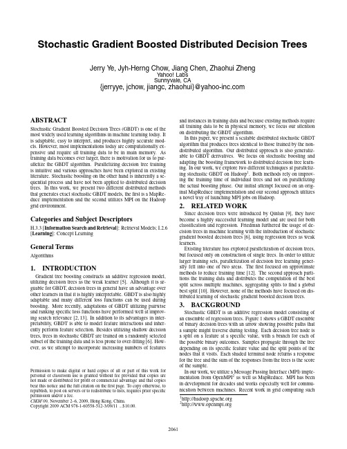
Stochastic Gradient Boosted Distributed Decision TreesJerry Y e,Jyh-Herng Chow,Jiang Chen,Zhaohui ZhengY ahoo!LabsSunnyvale,CA{jerryye,jchow,jiangc,zhaohui}@ABSTRACTStochastic Gradient Boosted Decision Trees(GBDT)is one of the most widely used learning algorithms in machine learning today.It is adaptable,easy to interpret,and produces highly accurate mod-els.However,most implementations today are computationally ex-pensive and require all training data to be in main memory.As training data becomes ever larger,there is motivation for us to par-allelize the GBDT algorithm.Parallelizing decision tree training is intuitive and various approaches have been explored in existing literature.Stochastic boosting on the other hand is inherently a se-quential process and have not been applied to distributed decision trees.In this work,we present two different distributed methods that generates exact stochastic GBDT models,thefirst is a MapRe-duce implementation and the second utilizes MPI on the Hadoop grid environment.Categories and Subject DescriptorsH.3.3[Information Search and Retrieval]:Retrieval Models;I.2.6 [Learning]:Concept LearningGeneral TermsAlgorithms1.INTRODUCTIONGradient tree boosting constructs an additive regression model, utilizing decision trees as the weak learner[5].Although it is ar-guable for GBDT,decision trees in general have an advantage over other learners in that it is highly interpretable.GBDT is also highly adaptable and many different loss functions can be used during boosting.More recently,adaptations of GBDT utilizing pairwise and ranking specific loss functions have performed well at improv-ing search relevance[2,13].In addition to its advantages in inter-pretability,GBDT is able to model feature interactions and inher-ently perform feature selection.Besides utilizing shallow decision trees,trees in stochastic GBDT are trained on a randomly selected subset of the training data and is less prone to over-fitting[6].How-ever,as we attempt to incorporate increasing numbers of features Permission to make digital or hard copies of all or part of this work for personal or classroom use is granted without fee provided that copies are not made or distributed for profit or commercial advantage and that copies bear this notice and the full citation on thefirst page.To copy otherwise,to republish,to post on servers or to redistribute to lists,requires prior specific permission and/or a fee.CIKM’09,November2–6,2009,Hong Kong,China.Copyright2009ACM978-1-60558-512-3/09/11...$10.00.and instances in training data and because existing methods require all training data to be in physical memory,we focus our attention on distributing the GBDT algorithm.In this paper,we present a scalable distributed stochastic GBDT algorithm that produces trees identical to those trained by the non-distributed algorithm.Our distributed approach is also generaliz-able to GBDT derivatives.We focus on stochastic boosting and adapting the boosting framework to distributed decision tree learn-ing.In our work,we explore two different techniques at paralleliz-ing stochastic GBDT on Hadoop1.Both methods rely on improv-ing the training time of individual trees and not on parallelizing the actual boosting phase.Our initial attempt focused on an orig-inal MapReduce implementation and our second approach utilizesa novel way of launching MPI jobs on Hadoop.2.RELATED WORKSince decision trees were introduced by Qinlan[9],they have become a highly successful learning model and are used for both classification and regression.Friedman furthered the usage of de-cision trees in machine learning with the introduction of stochastic gradient boosted decision trees[6],using regression trees as weak learners.Existing literature has explored parallelization of decision trees, but focused only on construction of single trees.In order to utilize larger training sets,parallelization of decision tree learning gener-ally fell into one of two areas.Thefirst focused on approximate methods to reduce training time[12].The second approach parti-tions the training data and distributes the computation of the best split across multiple machines,aggregating splits tofind a global best split[10].However,none of the methods have focused on dis-tributed learning of stochastic gradient boosted decision trees. 3.BACKGROUNDStochastic GBDT is an additive regression model consisting of an ensemble of regression trees.Figure1shows a GBDT ensemble of binary decision trees with an arrow showing possible paths that a sample might traverse during testing.Each decision tree node is a split on a feature at a specific value,with a branch for each of the possible binary outcomes.Samples propagate through the tree depending on its specific feature value and the split points of the nodes that it visits.Each shaded terminal node returns a response for the tree and the sum of the responses from the trees is the score of the sample.In our work,we utilize a Message Passing Interface(MPI)imple-mentation from OpenMPI2as well as MapReduce.MPI has been in development for decades and works especially well for commu-nication between machines.Recent work in grid computing such 12as the Apache Hadoop project have allowed for large scale deploy-ments of cheap,interchangeable compute nodes [4].Hadoop is an open source implementation of MapReduce [3]and it allows for streaming jobs where users can specify tasks for each compute node independent of MapReduce.In our work,we used MPI on Hadoop directly by writing a customized launcher.The next section describes how we distributed the training pro-cess for stochasticGBDT.Figure 1:A gradient boosted decision tree ensemble.4.METHODIn this section,we describe how to parallelize the stochastic GBDT learning process.Chen et.al.[2]presented a good overview of regression trees and gradient boosting in Section 3of TRADA.We describe various ways of partitioning the training data,our MapReduce implementation,and finally our MPI implementation on Hadoop.Before we proceed further,it is worth reiterating that we are only interested in learning exact models.The models are identical to those trained with the non-distributed version of the al-gorithm.This guided us as we made important design decisions.Alternatives to boosting and other tree ensemble methods such as random forests [11]were not attempted for this reason.4.1Distributed Training DataIn order to parallelize our decision tree training process,we must distribute the training data among machines.We are only interested in methods that would partition the data onto different machines rather than simply replicating it to reduce memory usage.There are already several existing approaches to distributed tree construction that aimed to improve scalability in terms of memory usage and improving training performance [8].Caregea et.al.outlined algo-rithms for distributed tree training and presented different methods for partitioning training data,either horizontally or vertically [1].In our work,we distributed our data using both vertically and hori-zontally partitioned methods.4.2MapReduce ImplementationOur initial implementation of distributed decision trees tried to frame the problem in the MapReduce paradigm and used a hori-zontal partitioning approach.Gehrke et.al.presented the concept of aggregating attribute,value,class label pairs and we utilized this in our MapReduce implementation [7].Mappers would collect suf-ficient statistics [1]for tree construction,where each computes the candidate cutpoints by aggregating the unique attribute-value pairs.Algorithm 1details the mapper and reducer code for finding candi-date split points.During the map phase,the sufficient statistics con-sist of a key (f,v ),containing the feature f and the feature value v ,and the corresponding value (r i ,w i )consisting of the current residual and the weight of sample i .The reduce phase aggregates the residual and weight sums for each key.Given the output file,we then perform a single pass over the sorted cutpoints and the global best cut can be found.This MapReduce method reduces the complexity of finding the optimal cutpoint for each feature from the dimension of the number of samples to the number of unique sample values.This method scales particularily well on datasets with categorical or Boolean features (e.g.click data).The entire process requires another mapAlgorithm 1Aggregating candidate splits map (key,value ):F ⇐set of featuressample ⇐split(value,delim)for f in F dokey =(f,sample[f])value =(sample[residual],sample[weight])emit(key,value)end for reduce (key,values ):residual_sum ⇐0weight_sum ⇐0for v in values doresidual_sum ⇐residual_sum +v.residual weight_sum ⇐weight_sum +v.weight end foremit(key,(residual_sum,weight_sum))Algorithm 2Partitioning a Node n map (key,value ):sample ⇐split(value,delim)if sample[n.feature]<n.splitpoint thenresidual =sample[residual]+n.left_response elseresidual =sample[residual]+n.right_response end ifemit(key,value)task to partition the data for each node and a final one to apply the current ensemble after training an entire tree.Algorithm 2shows pseudo code for updating the residuals for each sample.The par-titioner writes samples out to different output files depending on which side of the split the sample ends up.The applier code is trivial to write in MapReduce and is omitted.The MapReduce implementation is relatively straight forward to implement and requires few lines of code.However,because we essentially use HDFS for communication by writing out multiple files when splitting a node,we suffer from high system overhead.Hadoop is currently just not a good fit for this class of algorithms.Due to high communication overhead,we shift the focus of the remaining parts of this section to our MPI approach.4.3Learning a Distributed Regression Tree withMPI on HadoopOur second approach tries to optimize communication by using MPI on Hadoop streaming rather than MapReduce.For this im-plementation,we chose vertical partitioning since it minimizes the communication overhead of computing a tree node.For the rest of the paper,we will be working with vertically partitioned data,unless otherwise noted.Load balancing was performed to reduce time spent waiting for stragglers.For our implementation,we used our own MPI launcher for Hadoop.4.3.1MPI on HadoopIn order to utilize existing Hadoop clusters,we modified Open-MPI to launch using Hadoop streaming.The main advantage of our approach is that we can use existing clusters without having to build out a dedicated MPI cluster.Technical challenges such as determining and communicating the master node,SSH-less job launching,and fault tolerance had to be solved in the process.4.3.2Finding the Best Split for a NodeThe best split for a node is the split c i,j that maximizes gain(c) across all unique cut points j and feature i∈F,where F is the set of all features.For vertical partitioning,each machine works on a subset of the feature space F L and have only enough information to compute the best local split S i,j for a unique cut point j and feature i∈F L.S i,j=argmax i,j{gain(c i,j)}Each machine computes the best gain among its subset of features and sends this information to all of the other machines using an MPI broadcast.Each machine then determines the global best split S∗i,j by aggregating the local splits from each machine and deter-mining which split S i,j corresponds to the cut point c i,j that maxi-mizes gain.S∗i,j=argmax i,j{gain(c i,j)}Every machine now knows the global best cut and waits for the machine with the split feature in memory to partition its samples and then transmit the updated post-split indices.4.3.3Partitioning the DataDuring traditional decision tree construction,samples are parti-tioned into two subsets after a split point is learned.In distributed partitioning,only one machine has the feature in memory to parti-tion the dataset.Therefore,only the machine with the best split can partition the data,updating other machines after it isfinished.In stochastic GBDT,we start off with a random subset of the training data for each tree.Since the targets for each sample in the next tree is the gradient of the loss function,we need the current score for every sample in the training set during boosting.This poses a unique problem in the distributed case where we have to apply the current ensemble on samples with features distributed on multiple machines.To remedy this,we modify our partition process to operate over all samples in the training data and maintain an incremental score indexscore m(x)=score m−1(x)+J mXj=1γjm I(x∈R jm)where the current score at tree m depends on the score of the sample from training the previous m−1trees,the indicator func-tion,I and the responseγjm of the corresponding region if x is in region R jm.Since the response is the residual mean of samples at the inner nodes of the tree,we can incrementally update the score index as we train new nodes.The additional overhead at each tree is inversely linear with the sampling rate.4.3.4Finding the Best Node for SplittingWe employ the same greedy tree growing procedure that splits the node with the highest gain among current leaf nodes.Although this does not guarantee the optimal tree,it is an efficient linear pro-cess and follows the method used in our non-distributed version. Other tree growing methods can be implemented with additional parallelism,such as growing by level,but in the interest of attaining identical trees,we opted to use the greedy process.4.4Stochastic Gradient Boosting withDistributed Decision TreesGradient Boosted Decision Trees is an additive regression model consisting of numerous weak decision tree learners h i(x).H k(x)=kXi=1γi h i(x)whereγi denotes the learning rate.In Stochastic Gradient Boost-ing,each weak learner h i(x)is trained on a subsample of the train-ing data.Normally,during sequential training,the target t i of sample x i for the k-th tree is the gradient of the loss function L(y i,s i),usu-ally with parameters y i being the true label of the sample and the score s i=H k−1(x i).The loss function could be as generic as least squares or as specialized as GBRank[13].A unique challenge occurs when training distributed decision trees where data is partitioned across multiple nodes.Since the loss function depends on the score of every sample in the training data for the ensemble thus far,we need to retrieve non-local fea-ture values from other machines or keep track of the sample score throughout training.Our method implements the latter to minimize communication between machines.Therefore,during training,we modify our applier function to beH k(x)=s k(x)where s k(x)is the index described in Section4.3.3,with s0(x)= 0.Boosting then follows as shown below:1.Randomly sample the training data with replacement to getsubset S k.2.Set the target r i of examples in S k to be r i=L(y i,s k(x i))where y i is the true label of the sample3.Train the k-th tree h k(x)with the samples(x i,ri),wherex i∈S k.5.EXPERIMENTSThis section overviews the results of our experiments.Since our distributed GBDT construction process is designed to produce ex-actly the same results as the non-distributed version,we do not need to evaluate for differences in accuracy between learned models.We focus solely on evaluating performance and scalability of our sys-tems.Wefirst describe our dataset and experimental setup,then the results of our MapReduce implementation.Finally,we discuss the results of our implementation utilizing MPI on Hadoop.5.1Experimental SetupOur experiments focused on evaluating the scalability of our sys-tems when more machines are added to the process or when the feature or sample size is varied.All runs were made on a Hadoop cluster with only the number of machines allocated as needed. The dataset D used in our experiments consisted of1.2million (query,uri,grade)samples with520numeric features.To stress the system,we randomly generated,while respecting the existing feature distributions,additional datasets that were multiples of the dimension of D.5.2Experimental Results5.2.1MapReduce ImplementationFigure2is a log-log plot of training times for training a decision tree node.For each of the datasets,we trained a tree and aver-aged the training time for splitting a node,partitioning the samples, and updating the residuals for its children.As expected,the larger1000500100510050 105T r a i n i n g T i m e (s e c o n d s )Number of Machines1.2 Million150KFigure 2:Training time per node using the MapReduce implementation shown in log scale.dataset saw the largest improvement in training time as more map-pers were added.Due to communication overhead,there were no further performance gains on the smaller dataset after 50machines were used.Communication costs were the main concern with this imple-mentation.We discovered that this process was restricted by high cost of communication across HDFS (Hadoop currently does not have support for inter-node communication).Scheduling of multi-ple MapReduce jobs also proved to be a costly proposition.Given these factors,we were looking at minutes per node.This implemen-tation was actually slower than the non-distributed version.From our results,we believe that MapReduce is simply not a good fit for communications heavy algorithms such as GBDT and highly iterative machine learning algorithms in general.Although our MapReduce implementation scales well with even larger datasets,we were primarily interested in improving over-all training time and changed our focus to using MPI on paratively,the MPI implementation trains an entire 20termi-nal node tree in only 9seconds with 20machines on the 1.2M sam-ple dataset while the MapReduce implementation took 273seconds to train a single node with 100machines.5.2.2MPI Implementation.To evaluate the scalability of our MPI system,we used three dif-ferent datasets of varying sizes consisting of 1.2million samples,500K samples,and 100K samples each.There were 520features across all three datasets.For each dataset,we learned 10trees with each tree trained until there were 20leaf nodes.We repeated this experiment multiple times as we varied the number of machines during our distributed training process.Figure 3shows a log-log plot of the average training time as a function of the number of machines.The graph shows that the speedups depend on the size of the training data and that improve-ments start to taper off as more machines are added.In our dataset with 100K samples,the overhead from distributed tree training was too high for our implementation to be useful.For the 500K dataset,training time was reduced in half after using 2machines but contin-ued to improve sub-linearly until 5machines were used and having no further improvements from additional machines.The biggest advantage to using our implementation came with the larger 1.2million sample dataset.We see that training time is halved by adding an additional machine and that improvements continue up to 20machines with the final improvement from 70seconds per tree to 9seconds per tree.Figure 3appears to indicate that we should be able to obtain even better scaling as our dataset grows larger.We gained a lot in terms of performance using the MPI approach,but we lost some of the scalability afforded to us in the MapReduceimplementation.Because we focused on minimizing inter-machine communication,we decided to go with a vertical partitioning of our dataset.Although most datasets have many features and will benefit from the scalability of this implementation,we do reach an upper limit when the size of one feature cannot fit in main memory on one machine.1102010 5 4 3 2 1T r a i n i n g T i m e (s e c o n d s )Number of Machines1.2 Million500K 100KFigure 3:Average training time per tree over 10trees shown in log scale.6.CONCLUSIONSWe have shown two different methods of parallelizing stochastic gradient boosted decision trees.Our first implementation follows the MapReduce paradigm and ran on Hadoop.This approach re-quired a very limited amount of code and scaled well.However,communication costs of reading from HDFS was too expensive for this method to be useful.In fact,it was slower than the sequential version.We believe that the main factor behind the results was that our communication intensive implementation is not well suited for the MapReduce paradigm.Our second method utilizes MPI and Hadoop streaming to run on the grid.This approach proved to be successful,obtained near ideal speedups,and scales well with large datasets.7.REFERENCES [1]C ARAGEA ,D.,S ILVESCU ,A.,AND H ONAVAR ,V.A framework for learningfrom distributed data using sufficient statistics and its application to learning decision trees.International Journal of Hybrid Intelligent Systems 1,2(2004).[2]C HEN ,K.,L U ,R.,W ONG ,C.K.,S UN ,G.,H ECK ,L.,AND T SENG ,B.L.Trada:tree based ranking function adaptation.In CIKM (2008),pp.1143–1152.[3]D EAN ,J.,AND G HEMAWAT ,S.Mapreduce:simplified data processing on large mun.ACM 51,1(2008),107–113.[4]F OUNDATION ,A.Apache hadoop /hadoop .[5]F RIEDMAN ,J.H.Greedy function approximation:A gradient boosting machine.Annals of Statistics 29(2001),1189–1232.[6]F RIEDMAN ,J.H.Stochastic gradient put.Stat.Data Anal.38,4(February 2002),367–378.[7]G EHRKE ,J.,R AMAKRISHNAN ,R.,AND G ANTI ,V.Rainforest -a framework for fast decision tree construction of large datasets.In VLDB’98,Proceedings of 24rd International Conference on Very Large Data Bases,August 24-27,1998,New York City,New York,USA (1998),A.Gupta,O.Shmueli,and J.Widom,Eds.,Morgan Kaufmann,pp.416–427.[8]P ROVOST ,F.,K OLLURI ,V.,AND F AYYAD ,U.A survey of methods for scaling up inductive algorithms.Data Mining and Knowledge Discovery 3(1999),131–169.[9]Q UINLAN ,J.R.Induction of decision trees.In Machine Learning (1986),pp.81–106.[10]S HAFER ,J.C.,A GRAWAL ,R.,AND 0002,M.M.Sprint:A scalable parallel classifier for data mining.In VLDB’96,Proceedings of 22th International Conference on Very Large Data Bases,September 3-6,1996,Mumbai(Bombay),India (1996),T.M.Vijayaraman,A.P.Buchmann,C.Mohan,and N.L.Sarda,Eds.,Morgan Kaufmann,pp.544–555.[11]S TATISTICS ,L.B.,AND B REIMAN ,L.Random forests.In Machine Learning (2001),pp.5–32.[12]S U ,J.,AND Z HANG ,H.A fast decision tree learning algorithm.In AAAI (2006).[13]Z HENG ,Z.,C HEN ,K.,S UN ,G.,AND Z HA ,H.A regression framework for learning ranking functions using relative relevance judgments.Proceedings of the 30th annual international ACM SIGIR conference on Research and development in information retrieval (2007),287–294.。

第 42 卷第 3 期2023年 5 月Vol.42 No.3May 2023中南民族大学学报（自然科学版）Journal of South-Central Minzu University（Natural Science Edition）基于WGBDT的心衰患者半年内再入院风险预测徐瑞1，肖海军1，胡琛2*（1 中国地质大学数学与物理学院，武汉430074；2 华中科技大学同济医学院附属同济医院儿科学系，武汉430030）摘要为了解决现有心衰患者再入院风险预测评估模型缺乏可解释性、无法满足临床应用要求的问题，提出了一种基于自适应加权的梯度提升决策树（Weighted Gradient Boosting Decision Trees， WGBDT）的心衰患者半年内再入院风险预测模型.这一模型由基于WGBDT算法的风险预测和基于可解释机器学习（SHapley Additive exPlanation， SHAP）模型的解释性框架构成.其一，WGBDT风险模型通过样本权重更新来完成基分类器的训练.对通过基分类器分类误差率更新的残差样本进行迭代训练的基分类器加权累加，可以获得泛化性和准确率更好的模型；其二，SHAP可解释性框架采用Kernel SHAP和临床医学先验知识相结合的方式，对WGBDT黑箱模型进行解释，完成该模型的可解释性.使用四川省某医院的2008例心衰患者临床数据集对模型进行训练与测试，结果显示：利用该模型获得的结论优于梯度提升决策树（GBDT）、XGBoost、支持向量机、决策树、Adaboost等主流的机器学习算法获得的结论；同时，利用 SHAP框架提高了该模型的可解释性，并根据特征的重要性，识别出了影响心衰因素的重要性排序，这为医生制定更加合理的决策提供了科学的参考.关键词心衰；再入院；梯度提升决策树；样本权重；可解释机器学习模型中图分类号R541.6 文献标志码 A 文章编号1672-4321（2023）03-0425-08doi：10.20056/ki.ZNMDZK.20230320WGBDT-based risk prediction for readmission within six months inheart failure patientsXU Rui1，XIAO Haijun1，HU Chen2*（1 School of Mathematics and Physics， China University of Geosciences， Wuhan 430074， China；2 Department of Pediatrics， Tongji Hospital， Tongji Medical College， Huazhong University ofScience and Technology， Wuhan 430030， China）Abstract In order to solve the problem that existing models for predicting and assessing the risk of readmission in heart failure patients lack interpretability and cannot meet the requirements of clinical application，a WGBDT（Weighted Gradient Boosting Decision Trees）-based model for predicting the risk of readmission in heart failure patients within six months is proposed. This model consists of a risk prediction based on the WGBDT algorithm and an interpretation framework based on the SHAP（SHapley Additive exPlanation） model. On the one hand， the WGBDT risk model completes the training of the base classifier by updating the sample weights. The weighted accumulation of the base classifier that iteratively trains the residual samples updated by classification error rates of the base classifier can obtain a model with better generalization and accuracy. On the other hand， the SHAP interpretability framework uses a combination of Kernel SHAP and clinical medicine prior knowledge to interpret the WGBDT black box model and complete the interpretability of the proposed model. By using a clinical dataset with 2008 heart failure patients from a hospital in Sichuan Province as training set and test set， the results show that the conclusions obtained by the proposed model outperform those obtained by mainstream machine learning algorithms such as GBDT，XGBoost，SVM，DT，Adaboost ，et al. At the same time，the收稿日期2022-09-20* 通信作者胡琛（1992-），女，临床技师，博士，研究方向：环境流行病学，E-mail：******************基金项目国家自然科学基金资助项目（11901543）；国家级外专资助项目（华科专字G2021154019L）第 42 卷中南民族大学学报（自然科学版）interpretability of the proposed model is enhanced by using the SHAP framework and the order of the importance of factors affecting heart failure is identified according to the importance of the features. These provide a scientific reference for doctors to formulate more reasonable treatment plans.Keywords heart failure； readmission； Gradient Boosting Decision Trees； sample weights； SHapley Additive exPlanation心力衰竭（heart failure，简称心衰）的高再入院率与高医疗成本目前是各国普遍面临的问题.高效精准的风险评估能大大节省医疗成本，让心衰预后管理更具侧重性，所以对心衰患者再入院风险的准确评估成为了降低患者再入院率和节省医疗成本的关键.国内外已有学者相继建立并发布了大量再入院风险预测模型.现阶段主要使用两种心衰相关的风险预测模型：一是结合医学与统计学的传统模型，二是从机器学习方向出发的预后模型.在医学和统计学领域里，常用的有Logistic回归模型和Cox比例风险回归模型.然而地区的差异和截尾数据的影响会在一定范围内限制其推广和应用.近年来由于大数据服务与技术的迅速发展，并行计算效率的快速提升使机器学习被大量运用于医疗领域.国内外有学者利用机器学习算法对医疗数据进行建模：GOLAS等［1］建立心衰患者出院后30 d 全因再入院的深度学习风险预测模型，该模型分类准确率为76.4%；李金林等［2］采用神经网络、随机森林和支持向量机算法构建了10个再入院风险模型，使用多项式和函数的支持向量机模型的表现最好.许源等［3］利用XGboost对缺血性脑卒中患者90 d内再入院预测模型，与传统的Logistic回归分析模型相比，XGboost模型的风险预测效果更好.林瑜等［4］基于集成学习方法AdaBoost、GBDT等建立ICU预测模型，与Logistic回归分析模型对比，基于集成学习的预测模型有更好的表现.机器学习模型具有其独特的优势，对原始数据无较高要求，同时具有很强的自组织、自适应能力，但机器学习模型作为黑匣子只能实现数据到预测结果的映射，缺乏一定可解释性，这在一定程度上限制了此类模型在可解释性要求较高的医疗领域的应用.综上，针对心衰患者再入院风险预测领域，传统的统计学模型对数据的要求太高、对数据异常值较为敏感，机器学习尽管可以在一定程度上克服统计学模型局限性，但其可解释性较低，因此，考虑GBDT模型具有可抑制数据敏感性的特点，本文提出基于GBDT模型的心衰患者再入院风险预测模型，同时结合SHAP模型对GBDT模型进行因果分析，提高分类预测模型的可解释性.用基于自适应加权的GBDT方法（WGBDT）建立心衰患者再入院风险预测模型，WGBDT方法利用残差加权改变每次迭代后各个样本的权重来提升最终强分类器的分类性能.通过建立SHAP模型结合医学知识对WGBDT模型进行分析，使得WGBDT 预测模型变得更加具有解释性，同时得到比GBDT 算法更好的分类结果.通过仿真实验的结果证明：WGBDT算法相较于其他的算法具有更优的性能. 1　基于WGBDT的再入院风险预测模型1.1　模型原理1.1.1　GBDT理论GBDT于2001年由FRIEDMAN提出［5］，是一个以提升方法为框架的加法模型集成学习算法.在GBDT模型中常选用CART回归树作为基分类器，每一棵树的生成都是基于上一个回归树分类结果的残差，以串行的方式向残差减小的方向梯度迭代，最后累加所有树的结果加权求和作为最终结果. GBDT算法的流程如下.步骤1，取训练集T={(x1，y1)，(x2，y2)，…，(x n，y n)}，迭代次数M和损失函数L，初始化弱分类器F0(x)：F0(x)=arg minγ∑i=1n L(y i，γ).（1）步骤2，建立M棵分类回归树m=1，2，…，M：（1）对i=1，2，…，n，计算第m棵树对应的响应值（损失函数的负梯度，即伪残差）：rm，i=-[∂L(y i，F(x i))∂F(x)]F(x)=F m-1(x).（2）（2）对于i=1，2，...，n，利用CART回归树拟合数据(x i，r m，i)，得到第m棵回归树，其对应的叶子节点区域为R m，j，其中j=1，2，…，J m，且J m为第m棵回归树叶子节点的个数.（3）在J m个叶子节点区域j=1，2，…，J m，计算最优拟合值：cm，j=arg minγ∑x i∈R m，j L(y i，F m-1(x i)+γ).（3）更新强学习器F m(x)：426第 3 期徐瑞，等：基于WGBDT 的心衰患者半年内再入院风险预测F m (x )=F m -1(x )+∑j =1J mc m ，j I (x ∈R m ，j )，（4）其中，I (x ∈R m ，j )={1，x ∈R m ，j0，x ∉R m ，j.步骤3，最后得到的强学习器F M (x )的表达式：F M (x )=F 0(x )+∑m =1M∑j =1J mc m ，j I (x ∈R m ，j ).（5）1.1.2　改进GBDT 理论对于GBDT ，其每轮迭代拟合的样本是上一轮拟合的负梯度，也就是残差的近似值，而在训练过程中所有样本的权重始终相同，这就导致在训练时基学习器不能将注意力集中到难分样本上，使得分类结果不够精确.本文应用结合自适应样本加权思想和GBDT 算法能实现更好的模型分类性能.主要是每拟合完一棵树，通过Sigmoid 函数得到每个样本预测的可靠度；在分类开始阶段存在较多的误分类样本和难分样本，根据自适应样本加权的思想，对于易分样本缩小其样本权重，对于误分类样本和难分样本则增大其权值.在更新权重时用到了残差误差率和基分类器误差率，根据上一轮误差率来更新下一轮的残差样本权重.第m 棵树第i 个样本的残差误差率为：e m ，i =(r m ，i -∑j =1J mc m ，j I (x i ∈R m ，j ))2E m2.（6）其中E m 是拟合的残差中最大误差，E m =max i =1，2，…，n ||r m ，i -∑j =1J mc m ，j I (x i ∈R m ，j )||.（7）第m 个弱学习器的误差率定义如下：e m =∑i =1Nw m ，i ⋅e m ，i .（8）第m +1轮残差样本的权重定义如下：W m +1=(w m +1，1，w m +1，2，…，w m +1，n )，（9）w m +1，i =u m ，i∑i =1Nu m ，i ，（10）其中，残差权重因子：u m ，i =w m ，i ⋅(e m1-e m)1-e m ，i，i =1，2，…，n .（11）该改进算法的流程图如图1所示.1.2　再入院风险预测模型的实现本文再入院风险模型整体实现流程如图2所示，分为数据处理、特征工程、模型性能验证和SHAP 模型解释四个部分.2　实验结果分析2.1　实验配置和评价指标本文在节点CPU 为AMD R7-5700U 1.80 GHz 的Windows10系统上运行Python 3.8.8进行实验，其中Scikit -learn 库为1.1.1版本，编译环境为JupyterNotebook 6.4.11.混淆矩阵（如表1所示）是评价模型结果的指标，属于模型评估的一部分.基于混淆矩阵，可以衍生出一系列机器学习评价指标：准确率（Accuracy ，Acc ）、灵敏度（Sensitivity ，Sen ）、特异度（Specificity ，Spe ）、F1值和AUC 值，本文使用以上5个指标来进行评估.准确率为总的正确预测的样本数量占总样本数量的比值；灵敏度也叫召回率，表示正确预测的阳性样本占总阳性样本的比值；特异度表示正确预测的阴性样本占总阴性样本的比值；F1值为精确率和召回率的调和平均；AUC 是用构图法解释灵敏度和特异度的相互关系，曲线下面积越接近1，模型精度越高.上述指标公式分别如式（12）~（15）所示.Acc =TP +TNTP +TN +FP +FN，（12）图1 WGBDT 算法流程Fig. 1　Flow chart of WGBDT algorithm427第 42 卷中南民族大学学报（自然科学版）Sen =TPTP +FN，（13）Spe =TNTN +FP ，（14）F1=2TP2TP +FN +FP.（15）2.2　数据来源与处理2.2.1　数据来源及介绍本文数据［6-7］来源于四川自贡某医院2016―2019年的回顾性心力衰竭数据集.该数据集包括心力衰竭患者个案2008例，其中半年后复发的个案773例，半年后未复发的个案1235例.还包括涉及到患者基本资料、生命体征、基础疾病、神志反应、器官状态、实验室检查、常见抗心衰药物使用等7个方面的168个变量.为方便起见，下文中将半年后再入院和半年后未再入院统一简称为再入院和未再入院.2.2.2　数据预处理针对原始数据中的数据类型不统一、数据缺失、数据冗余等问题进行数据清洗，主要包括以下几个步骤：（1）数据量化处理.数据集中存在不少字符串形式的类别型特征，为了统一数据类型，需要对这些特征数据用LabelEncoder 进行转换.例如，年龄段分为了8个阶段，分别用｛1，2，3，…，7，8｝来表示.最终转换了15个类别型特征.（2）缺失值处理.可视化数据集的缺失值，结果如图3所示.白色代表数据缺失，白色越多表示数据缺失的越多。

常用英语词汇Andrew Ng课程intensity 强度Regression 回归Loss function损失函数non-convex非凸函数neural network 神经网络supervised learning 监督学A) regression problem回归问题处理的是连续的问题classification problem 分类问题discreet value 离散值autoencoder自编码器Autoencoders自编码算法average firing rate 平均激活率average sum-of-squares error 均方差backpropagation 后向传播basis 基basis feature vectors 特征基向量batch gradient ascent批量梯度上升法Bayesian regularization method 贝叶斯规则化方法Bernoulli random variable 伯努利随机变量support vector machines 支持向量机learning theory 学习理论learning algorithms 学习算法unsupervised learning 无监督学习gradient descent 梯度下降linear regression 线性回归Neural Network 神经网络gradient descent 梯度下降normal equations linear algebra 线性代数bias term偏置项binary classfication 二元分类class labels 类型标记concatenation 级联conjugate gradient 共範梯度contiguous groups 联通区域convex optimization software 凸优化软件convolution 卷枳cost function代价函数covariance matrix 协方差矩阵superscript 上标exponentiation 指数training set训练集合training example 训练样本hypothesis假设，用来表示学习算法的输出LMS algorithm "bast mean squares 最小二乘法算法batch gradient descent 批量梯度下降constantly gradient descent 随机梯度下降iterative algorithm 迭代算法partial derivative 偏导数contour等高线quadratic function 二元函数locally weighted regression 局部加权回归underfitting 欠拟合overfitting 过拟合non-parametric learning algorithms 无参数学习算法parametric learning algorithm 参数学习算法activation 激活值activation function 激活函数additive noise 加性噪声DC component宜流分量decorrelation去相关degeneracy 退化demensionality reduction 降维derivative 导函数diagonal对角线diffusion of gradients 梯度的弥散eigenvalue 特征值eigenvector特征向量error term 残差feature matrix 特征矩阵feature standardization 特征标准化feedforward architectures 前馈结构算法feedforward neural network 前馈神经网络feedforward pass 前馈传导fine-tuned 微调first-order feature —阶特征forward pass 前向传导forward propagation 前向传播Gaussian prior高斯先验概率generative model 生成模型gradient descent 梯度下降Greedy layer-wise training逐层贪婪训练方法grouping matrix 分组矩阵Hadamard product阿达马乘积Hessian matrix Hessian 矩阵hidden layer 隐含层hidden units隐藏神经元Hierarchical grouping 层次型分组higher-order features 更高阶特征highly non-c on vex op timization p roblem高度非凸的优化问题histogram直方图hyperbolic tangent双曲正切函数hypothesis估值，假设identity activation function 恒等激励函数110独立同分布illumination 照明inactive 抑制independent componentanalysis 独立成份分析overallcostfunction 总体代价函数over-complete basis 超完备基over-fitting 过拟合parts of objects目标的部件part-whole decompostion 部分•整体分解PCA主元分析penalty term惩罚丙子per-example meansubtraction 逐样本均值消减pooling 池化pretrain预训练linear superposition 线性叠加line-search algorithm 线搜索算法local mean subtraction 局部均值消减local optima局部最优解logistic regression 逻辑回归loss function损失函数low-pass filtering 低通滤波magnitude 幅值MAP极大后验估计maximum likelihood estimation 极大似然估讣principal compone nts an a lysis 主成份分析quadratic constraints 二次约束RBMs 受限Boltzman 机reconstruction based models 基于重构的模型rQConstruction cost 重建代价reconstruction term 重构项redundant 冗余reflection matrix 反射矩阵regularization 正则化regularizationterm 正则化项mean平均值MFCC Mel倒频系数multi-classclassification 多元分类neuralnetworks 神经网络neuron神经元Newton's method 牛顿法non-convexfunction 非凸函数non-linearfeature 非线性特征norm范式norm bounded有界范数norm constrained 范数约束normalization 归一化numerical roundoff errors 数值舍入误差numerically checking 数值检验numerically reliable数值汁算上稳世object detection 物体检测objective function 目标函数off-by-one error 缺位错误orthogonalization 正交化output layer 输出层input domains 输入感input layer 输入层intensity亮度/灰度intercept term 截距KL divergence 相对爛KL divergence KL 分散度k-Means K•均值learning rate 学Al 速率least squares 最小二乘法linear correspondence 线性响应rescaling 缩放robust鲁棒性run行程second-order feature 二阶特征sigmoid activation function S 型激励函数significant digits 有效数字singular value 奇异值singular vector 奇异向量smoothed LI penalty平滑的LI范数惩罚Smoothed topographic LI sparsity penalty translation invariant 平移不变性trivialanswer 平凡解under-complete basis 不完备基unrolling组合扩展unsupervised learning无监督学习variance 方差vecotrized implementation 向量化实现vectorization 矢量化visual cortex视觉皮层weight decay权重衰减weighted average加权平均值whitening 白化zero-mean均值为零Accumulated error backpropagation 累积误差逆传播Activation Function 激活函数Adaptive Resonance Theory/ART 自适应谐振理论Addictive model 加性学习Adversarial Networks 对抗网络Affine Layer 仿射层Affinity matrix 亲和矩阵squared-error 方差stationary平稳性（不变性）stationary stochastic process 平稳随机过程step-size步长值supervised learning 监督学习symmetric positive semi-definite matrix对称半正泄矩阵symmetry breaking 对称失效tanh function双曲正切函数the average activation 平均活跃度the derivative checking method 梯度验证方法the empirical distribution 经验分布函数the energy function 能量函数the Lagrange dual拉格朗日对偶函数the log likelihood对数似然函数the pixel intensity value 像素灰度值the rate of convergence 收敛速度topographic cost term 拓扑代价项topographie ordered 拓扌卜秩序transformation 变换Agent代理/智能体Algorithm 算法Alpha-beta pruning a-p 剪枝Anomaly detection 异常检测Approximation 近彳以Area Under ROC Curve / AUC Roc 曲线下而枳Artificial General Intelligence/AGI 通用人工智能Artificial Intelligence/Al 人工智能Association analysis 关联分析Attention mechanism 注意力机制Attribute conditional independence assumption属性条件独立性假设Attribute space 属性空间Attribute value 属性值Autoencoder自编码器Automatic speech recognition 自动语音识别Automatic summarization 自动摘要Average gradient 平均梯度Average-Pooling 平均池化Backpropagation Through Time通过时间的反向传播平滑地形LI稀疏惩罚函数smoothing 平滑Softmax Regresson Softmax 回归sorted in decreasing order 降序排列source features 源特征sparse autoencoder V 肖减—（fc Sparsity稀疏性sparsity parameter 稀疏性参数sparsity penalty 稀疏惩罚square function 平方函数Backpropagation/BP 反向传播Base learner基学习器Base learning algorithm 基学习算法Batch Normalization/BN 批量归一化Bayes decision rule贝叶斯判定准则Bayes Model Averaging / BMA 贝叶斯模型平均Bayes optimal classifier贝叶斯最优分类器Bayesian decision theory 贝叶斯决策论Bayesian network贝叶斯网络Between-class scatter matrix 类间散度矩阵Comprehensibility 可解释性Computation Cost i|•算成本Computational Linguistics 计算语•言学Computer vision讣算机视觉Concept drift概念漂移Concept Learning System /CLS 概念学习系统Conditional entropy 条件爛Conditional mutual information 条件互信息Conditional Probability Table / CPT 条件槪率表Conditional random field/CRF 条件随机场Bias偏置/偏差Bias-variance decomposition 偏差•方差分解Bias-Variance Dilemma 偏差-方差困境Bi-directional Long-Short Term Memory/Bi-LSTM 双向长短期记忆Binary classification 二分类Binomial test 二斯i检验Bi-partition 二分法Boltzmann machine 玻尔兹曼机Bootstrap sampling自助采样法/可重复采样Bootstrapping 自助法Break-Event Point / BEP 平衡点Calibration 校准Cascade-Correlation 级联相关Categorical attribute 离散属性Class-conditional probability 类条件概率Classification and regression tree/CART 分类与回归树Classifier 分类器Class-imbalance类别不平衡Closed -form 闭式Cluster簇/类/集群Cluster analysis 聚类分析Clustering 聚类Clustering ensemble 聚类集成Co-adapting 共适应Coding matrix编码矩阵COLT国际学习理论会议Committee-based learning 基于委员会的学Al Competitive learning 竞争型学习Component learner 组件学＞J 器Conditional risk 条件风险Confidence 置信度Confusion matrix 混淆矩阵Connection weight 连接权Connectionism 连结主义Consistency —致性/相合性Contingency table 列联表Continuous attribute 连续属性Convergence 收敛Conversational agent 会话智能体Convex quadratic programming 凸二次规戈ijConvexity 凸性Convolutional neural network/CNN 卷积神经网络Co-occurrence 同现Correlation coefficient 相关系数Cosine similarity 余弦相似度Cost curve成本曲线Cost Function成本函数Cost matrix成本矩阵Cost-sensitive 成本敏感Cross entropy 交叉爛Cross validation 交叉验证Crowdsourcing 众包Curse of dimensionality 维数灾难Cut point截断点Cutting plane algorithm 割平而法Data mining数据挖掘Data set数据集Decision Boundary 决策边界Decision stump 决策树桩Decision tree决策树/判泄树Deduction 演绎Deep Belief Network深度信念网络Deep Convolutional Generative Adversarial Network DCGAN深度卷积生成对抗网络Deep learning深度学习Deep neural network/DNN 深度神经网络Deep Q^Learning 深度Q 学习Deep Q-Network 深度Q 网络Density estimation 密度估计Density-based clustering 密度聚类Differentiable neural computer 町微分神经i|•算机Dimensionality reduction algorithm 降维算法Directed edge 有向边Disagreement measure 不合度虽Discriminative model 判别模型Discriminator 为J别器Distance measure 距离度量Distance metric learning 距离度量学Aj Distribution 分布Error Correcting Out put Codes / ECOC 纠错输出码Error rate错误率Erronambiguity decomposition 误差•分歧分解Euclidean distance 欧氏距离Evolutionary computation 演化计算Expectation-Maximization 期望垠大化Expected loss期望损失Exploding Gradient Problem 梯度爆炸问题Exponential loss function 指数损失函数Extreme Learning Machine/ELM 超限学习机Factorization 因子分解False negative 假负类False positive 假正类False Positive Rate/FPR 假正例率Feature engineering 特征工程Feature selection 特征选择Feature vector 特征向量Featured Learning 特征学习Feedforward Neural Networks/FNN 前馈神经网络Fine-tuning 微调Divergence 散度Diversity measure多样性度量/差异性度量Domain adaption领域自适应Down sampling 下采样□-separation (Directed separation ) 有向分离Dual problem对偶问题Dummy node哑结点Dynamic Fusion 动态融合Dynamic programming 动态规划Eigenvalue decomposition 特征值分解Flipping output 翻转法Fluctuation 農荡Forward stagewise algorithm 前向分步算法Frequentist频率主义学派Fulkrank matrix 满秩矩阵Functional neuron 功能神经元Gain ratio增益率Game theory 博弈论Gaussian kernel function 高斯核函数Gaussian Mixture Model 高斯混合模型General Problem Solving 通用问题求解 Generalization 泛化 Generalization error 泛化误差Generalization error bound 泛化谋差上界 Generalized Lagrange function广义拉格朗日函数 Generalized linear model 广义线性模型Generalized Rayleigh quotient 广义瑞利商 Generative Adversarial Networks/GAN 生成对抗网络 Generative Model 生成模型 Generator 生成器Embedding 嵌入Emotional analysis 情绪分析Empirical conditional entropy 经验条件熾 Empirical entropy 经验箱 Empirical error 经验误差 Empirical risk 经验风险 End*to-End 端到端Energy-based model 基于能量的模型 Ensemble learning 集成学习集成修剪Inter-cluster similarity 簇间相似度International Conferenee for Machine Learning/ICML 国际机器学习大会Intra-clustersimilarity 簇内相似度Intrinsic value 固有值Isometric Mapping/lsomap 等度量映射Isotonic regression 等分回归Iterative Dichotomiser 迭代二分器Kernel method 核方法Kernel trick 核技巧Kernelized Linear Discriminant Analysis / KLDAHard voting 硬投票Harmonic mean调和平均Hesse matrix海塞矩阵Hidden dynamic model 隐动态模型Hidden layer 隐藏层Hidden Markov Model/HMM隐马尔可夫模型Hierarchical clustering 层次聚类Hilbert space希尔伯特空间Hinge loss function合页损失函数Hold-out留出法核线性判别分析K-fold cross validation k折交叉验证/ k倍交叉验证K-Means Clustering K -均值聚类K-Nearest Neighbours Algorithm/KNN K 近邻算法Knowledge base 知识库Knowledge Re presentation 知识表征Label space标记空间Lagrange duality拉格朗日对偶性Lagrange multiplier拉格朗日乘子Laplace smoothing拉普拉斯平滑Homogeneous 同质Hybrid computing 混合讣算HypQ中arameter超参数Hypothesis 假设Hypothesis test 假设验证ICML国际机器学习会议Improved iterative scaling/IIS 改进的迭代尺度法Incremental learning 增量学习Independent and identically distributed/ 独立同分Indicator function 指示函数Individual learner 个体学〉J器Induction 归纳Inductive bias 归纳偏好Inductive learning 归纳学习Inductive Logic Programming / ILP 归纳逻辑程序设计Information entropy 借息爛Information gain 信息増益Input layer 输入层Insensitive loss不敏感损失Genetic Algorithm/GA 遗传算法Gibbs sampling吉布斯采样Giniindex基尼指数Global minimum 全局最小GlobalOptimization 全局优化Gradientboosting 梯度提升GradientDescent 梯度下降Graph theory 图论Ground-truth 貞•相 / 真实Hard margin 硬间隔布Independent Component Analysis/ICA 独立成分分析Laplacian correction 拉普拉斯修正Latent Dirichlet Allocation 隐狄利克雷分布Latent semantic analysis 潜在语义分析Latent variable 隐变量Lazy learning懒惰学习Learner学习器Learning by analogy 类比学习Learning rate 学习率Learning Vector Quantization/LVQ 学习向量量化Least squares regression tree 最小二乘回归树Leave-One-Out/LOO 留一法linear chain conditional random field 线性链条件随机场Linear Discriminant Analysis / LDA 线性判别分析Linear model线性模型Linear Regression 线性回归Link function联系函数Local Markov property局部马尔可夫性Local minimum 局部最小Log likelihood 对数似然Log odds / logit 对数几率Logistic Regression Logistic 回归Log-likelihood 对数似然Log-linear regression 对数线性回归Long-Short Term Memory/LSTM 长短期记忆Loss function损失函数Machine translation/MT 机器翻译Macron-P宏查准率Macron-R宏査全率Majority voting绝对多数投票法Multilayer Perceptron/MLP 多层感知器Multimodal learning 多模态学Multiple Dimensional Seating 多维缩放Multiple linear regression 多元线性回归Multi-res ponse Lin ear Regressio n / MLR 多响应线性回归Mutual information 互信息Naive bayes朴素贝叶斯Naive Bayes Classifier朴素贝叶斯分类器Named entity recognition 命名实体识别Manifold assumption 流形假设Manifold learning 流形学Margin theory间隔理论Marginal distribution 边际分布Marginal independence 边际独立性Marginalization 边际化Markov Chain Monte Carlo/MCMC马尔可夫链蒙特卡罗方法Markov Random Field马尔可夫随机场Maximal clique 最大团Maximum Likelihood Estimation/MLE极大似然估计/极大似然法Maximum margin 最大间隔Maximum weighted spanning tree 最大带权生成树Max-Pooling最大池化Mean squared error 均方误差Meta-learner 元学Al 器Metric learning 度量学习Micro-P微査准率Micro-R微査全率Nash equilibrium 纳什均衡Natural language generation/NLG 自然语H生成Natural language processing 自然语n 处理Negative class 负类Negative correlation 负相关法Negative Log Likelihood 负对数似然Neighbourhood Component Analysis/NCA近邻成分分析Neural Machine Translation 神经机器翻译Neural Turing Machine 神经图灵机Newton method 牛顿法NIPS国际神经信息处理系统会议No Free Lunch Theorem / NFL没有免费的午餐世理Noise-contrastive estimation 噪音对比估计Nominal attribute 列名属性Non-convex optimization 非凸优化Nonlinear model非线性模型Non-metric distance 非度量距离Non-negative matrix factorization 非负矩阵分解Non-ordinal attribute 无序属性Minimal Description Length/MDL 最小描述长度Minimax game极小极大博弈Misclassification cost 误分类成本Mixture of experts 混合 $家Momentum 动量Moral graph逍徳图/端正图Multi-class classification 多分类Multi-document summarization 多文档摘要Multi-layer feedforward neural networks Non-Saturating Game 非饱和博弈Norm 范数Normalization 归一化Nuclear norm 核范数Numerical attribute 数值属性Letter 0Objective function 目标函数Oblique decision tree 斜决策树Occam^s razor 奥卡姆剃刀Odds几率多层前馈神经网络Off-Policy 离策略One shot learning —次性学习One-Dependent Estimator / ODE 独依赖估计On-Policy在策略Ordinal attribute 有序属性Out-of-bag estimate 包外估计Output layer 输出层Output smearing输出调制法Overfitting过拟合/过配Oversampling 过采样Quantized Neural Network It子化神经网络Quantum computer量子计算机Quantum Computing 量子计算Quasi Newton method 拟牛顿法Radial Basis Function ./ RBF 径向基函数Random Forest Algorithm 随机森林算法Random walk随机漫步Recall查全率/召回率Receiver Operating Characteristic/ROC受试者工作特征Paired t-test 成对t 检验Pairwise成对型Pairwise Markov property 成对马尔可夫性Parameter 参数Parameter estimation 参数估计Parameter tuning 调参Parse tree解析树Particle Swarm Optimization/PSO 粒子群优化算法Part-of-speech tagging 词性标注Perceptron 感知机Performance measure 性能度量Plug and Play Generative Network 即插即用生成网络Plurality voting相对多数投票法Polarity detection 极性检测Polynomial kernel function 多项式核函数Pooling 池化Positive class 正类Positive definite matrix 正定矩阵Post-hoc test后续检验Post-pruning 后剪枝再生核希尔伯特空间Re-sampling重采样法Rescaling再缩放Residual Mapping 残差映射Residual Network 残差网络Restricted Boltzmann Machine/RBM 受限玻尔兹曼机Restricted Isometry Property/RIP 限定等距性Re-weighting重賦权法Robustness稳健性/鲁棒性Root node根结点Potential function 势函数Precision査准率/准确率Prepruning 预剪枝Principal component analysis/PCA 主成分分析Principle of multiple explanations 多释原则Prior先验Probability Graphical Model 概率图模型Proximal Gradient Descent/PGD 近端梯度下降Pruning 剪枝Pseudo-label 伪标记Rule Engine规则引擎Rule learning 规则学nJSaddle point 鞍点Sample space样本空间Samp ling 采样Score function 评分函数Self-Driving自动驾驶Self-Organizing Map / SOM 自组织映射Semi-naive Bayes classifiers半朴素贝叶斯分类器Semi-Supervised Learning 半监督学习Rectified Linear Unit/ReLU 线性修正单元Recurrent Neural Network 循环神经网络Recursive neural network 递归神经网络Reference model 参考模型Regression 回归Regularization 正则化Reinforcement learning/RL 强化学习Representation learning 表征学习Representer theorem 表示窪理rep reducingkernel Hilbert sp ace/RKHSsemi-Supervised Support Vector Machine半监督支持向量机Sentiment analysis 情感分析Separating hyperplane 分离超平而Sigmoid function Sigmoid 函数Similarity measure 相似度度疑Simulated annealing 模拟退火Simultaneous localization and map ping 同步楚位与地图构建Singular Value Decomposition 奇异值分解Tensor张量Tensor Processing Units/TPU 张量处理单元The least square method 最小二乘法Threshold 阈值Threshold logic unit阈值逻辑单元Threshold-moving 阈值移动Time Step时间步骤Tokenization 标记化Training error 训练误差Training instance训练示例/训练例Slack variables 松弛变量Smoothing 平滑Soft margin 软间隔Soft margin maximization 软间隔最大化Soft voting 软投票Sparse representation 稀疏表征Sparsity稀疏性Specialization 特化Spectral Clustering 谱聚类Speech Recognition 语音识别Splitting variable 切分变量Squashing function 挤压函数Stability-plasticity dilemma 可塑性•稳企性困境Statistical [earning 统讣学Status feature function 状态特征函Stochastic gradient descent 随机梯度下降Stratified sampling 分层采样Structural risk 结构风险Structural risk minimization/SRM 结构风险最小化Subspace子空间Transductive learning 宜推学习Transfer learning 迁移学习Treebank 树库Tria-by-error 试错法True negative 負•负类TruQpositive 真正类True Positive Rate/TPR 真正例率Turing Machine 图灵机Twice-learning 二次学习Underfitting欠拟合/欠配Undersampling 欠采样Understandability 可理解性Unequal cost非均等代价Unit-step function单位阶跃函数Univariate decision tree 单变量决策树Unsupervised learning无监督学习/无导师学习Unsupervised layer-wise training 无监督逐层训练Up sampling 上采样Vanishing Gradient Problem 梯度消失问题Variational inference 变分推断Supervised learning监督学习/有导师学习suppo rt vector ex pan sion 支持向量展式Support Vector Machine/SVM 支持向量机Surrogat loss替代损失Surrogate function 替代函数Symbolic learning 符号学习Symbolism符号主义Synset同义词集T-Distribution Stochastic Neighbour Embedding t-SNET-分布随机近邻恢入VC Theory VC 维理论Version space版本空间Viterbi algorithm 维特比算法Von Neumann architecture 冯•诺伊曼架构Wasserstein GAN/WGAN Wasserstein 生成对抗网络Weak learner弱学习器Weight权重Weight sharing 权共享Weighted voting加权投票法Within-class scatter matrix 类内散度矩阵Word embedding 词嵌入Word sense disambiguation 词义消歧Zero-data learning 零数据学习Zero-shot learning 零次学习approximations 近似值arbitrary随意的affine仿射的arbitrary任意的amino acid氨基酸amenable经得起检验的concrete具体的事物.实在的东西cross validation 交叉验证correlation林I互关系convention 约左cluster 一簇centroids质心，形心converge 收敛computationally il•算（机）的calculus 计算derive获得.取得axiom公理•原则abstract 提取architecture架构，体系结构：建造业absolute绝对的arsenal军火库assignment 分配algebra 线性代数asymptotically 无症状的appropriate 恰当的bias偏差dual二元的duality二元性：二象性：对偶性derivation求导：得到；起源denote预示，表示，是…的标志：意味着，［逻］指称divergence散度；发散性dimension尺度，规格；维数dot小圆点distortion 变形density槪率密度函数discrete离散的brevity简短，筒洁：短暂［800 J broader 广泛briefly简短的batch批量convergence收敛，集中到一点convex凸的contours 轮廉constraint 约束constant 常理commercial 商务的discriminative有识别能力的diagonal 对角dispersion分散•散开determinant决定因素disjoint不相交的encounter 遇到ellipses tffiR equality 等式extra额外的empirical 经验；观察complementarity 补充coordinate ascent 同等级上升clipping剪下物；剪报：修剪component分虽：：部件continuous 连续的covariance 协方差canonical正规的，正则的concave非凸的corresponds相符合：相当；通信corollary 推论ennmerate例举，讣数exceed 超过•越出expectation 期望efficient生效的endow賦予explicitly 清楚的exponential family 指数家族equivalently 等价的feasible可行的forary初次尝试finite有限的，限世的forgo摒弃，放弃filter过滤frequentist垠常发生的forward search前向式搜索formalize使宅形generalized 归纳的generalization槪括，归纳；普遍化：判断（根据不足）guarantee保证：抵押品generate形成，产生geometric margins 儿何边界gap 裂口generative生产的；有生产力的heuristic启发式的：启发法：启发程序hone怀恋；磨hyperplane 超平而initial垠初的implement 执行intuitive凭直觉获知的incremental 增加的intercept 截距intuitious 直觉instantiation 例子indicator指示物，指示器interative重复的.迭代的integral 枳分identical相等的：完全相同的indicate表示.指出invariance不变性，恒定性impose把…强加于intermediate 中间的interpretation 解释，翻译joint distribution 联合概率lieu替代logarithmic对数的，用对数表示的latent潜在的Leave-one-out cross validation 留一法交叉验ilE magnitude 巨大mapping绘图，制图；映射matrix矩阵mutual相互的♦共同的monotonically 单调的minor较小的，次要的multinomial 多项的multi-class classification 二分类问题nasty讨厌的notation标志，注释naive朴素的obtain得到oscillate 摆动optimization problem 最优化问题objective function 目标函数optimal最理想的orthogonal!矢量，矩阵等）正交的orientation 方向ordinary普通的occasionally 然的partial derivative 偏导数Property 性质Proportional成比例的primal原始的，垠初的permit允许pseudocode 伪代码permissible可允许的polynomial 多项式preliminary 预备precision 精度perturbation 不安.扰乱poist假定，设想Positive semi-definite 半正世的parentheses 圆括号posterior probability 后验概率Plementarity 补充pictorially 图像的parameterize确定…的参数poisson distribution 柏松分布pertinent相关的quadratic 二次的quantity量，数量；分量query疑问的regularization使系统化：调整reoptimize重新优化restrict限制：限定:约束reminiscent回忆往事的：提醒的；使人联想...的（of） remark注意random variable 随机变量respect 考虑respectively各自的：分别的redundant ht多的；冗余的susceptible 敏感的stochastic町能的：随机的symmetric对称的sophisticated 复杂的spurious假的；伪造的subtract减去；减法器simultaneously同时发生地：同步地suffice 满足scarce稀有的，难得的split分解，分离subset子集statistic统讣量successive iteratious 连续的迭代scale 标度sort of有几分的squares 平方trajectory 轨迹temporarily 暂时的terminology专用名词tolerance容忍：公差thumb翻阅threshold 阈，临界theorem 定理tangent 正弦unit-length vector 单位向量valid有效的，正确的variance 方差variable变量：变元vocabulary 词汇valued经估价的：宝贵的wrapper 包装总计1038词汇。

GBDT算法原理深入解析标签：机器学习集成学习GBM GBDT XGBoost梯度提升（Gradient boosting）是一种用于回归、分类和排序任务的机器学习技术，属于Boosting算法族的一部分。

Boosting是一族可将弱学习器提升为强学习器的算法，属于集成学习（ensemble learning）的范畴。

Boosting方法基于这样一种思想：对于一个复杂任务来说，将多个专家的判断进行适当的综合所得出的判断，要比其中任何一个专家单独的判断要好。

通俗地说，就是“三个臭皮匠顶个诸葛亮”的道理。

梯度提升同其他boosting方法一样，通过集成（ensemble）多个弱学习器，通常是决策树，来构建最终的预测模型。

Boosting、bagging和stacking是集成学习的三种主要方法。

不同于bagging方法，boosting方法通过分步迭代（stage-wise）的方式来构建模型，在迭代的每一步构建的弱学习器都是为了弥补已有模型的不足。

Boosting族算法的著名代表是AdaBoost，AdaBoost算法通过给已有模型预测错误的样本更高的权重，使得先前的学习器做错的训练样本在后续受到更多的关注的方式来弥补已有模型的不足。

与AdaBoost算法不同，梯度提升方法在迭代的每一步构建一个能够沿着梯度最陡的方向降低损失（steepest-descent）的学习器来弥补已有模型的不足。

经典的AdaBoost算法只能处理采用指数损失函数的二分类学习任务，而梯度提升方法通过设置不同的可微损失函数可以处理各类学习任务（多分类、回归、Ranking等），应用范围大大扩展。

另一方面，AdaBoost算法对异常点（outlier）比较敏感，而梯度提升算法通过引入bagging思想、加入正则项等方法能够有效地抵御训练数据中的噪音，具有更好的健壮性。

这也是为什么梯度提升算法（尤其是采用决策树作为弱学习器的GBDT算法）如此流行的原因，有种观点认为GBDT是性能最好的机器学习算法，这当然有点过于激进又固步自封的味道，但通常各类机器学习算法比赛的赢家们都非常青睐GBDT算法，由此可见该算法的实力不可小觑。

User G uide f or t he M ODIS L and C over T ype P roduct (MCD12Q1)Last U pdated: A ug 8, 20121. IntroductionLand c over p lays a m ajor r ole i n t he c limate a nd b iogeochemistry o f t he E arth system. A n i mportant u se o f g lobal l and c over d ata i s t he i nference o f p arameters that i nfluence b iogeochemical a nd e nergy e xchanges b etween t he a tmosphere a nd the l and s urface f or u se i n m odels a nd o ther g lobal c hange s cience a pplications. Examples o f s uch p arameters i nclude l eaf a rea i ndex, r oughness l ength, s urface resistance t o e vapotranspiration, c anopy g reenness f raction, v egetation d ensity, root d istribution, a nd t he f raction o f p hotosynthetically-­‐active r adiation a bsorbed. The M ODIS L and C over T ype P roduct p rovides a s uite o f l and c over t ypes t hat support g lobal c hange s cience b y m apping g lobal l and c over u sing s pectral a nd temporal i nformation d erived f rom M ODIS. T he o bjective o f t his d ocument i s t o provide i nformation r elated t o t he C ollection 5 M ODIS L and C over T ype P roduct (MCD12Q1). I t i s n ot d esigned t o b e a s cientific d ocument. R ather, i t p rovides t hree main t ypes o f i nformation:1.An o verview o f t he M CD12Q1 a lgorithm a nd p roduct, a long w ith r eferencesto p ublished l iterature w here m ore d etails c an b e f ound.2.Guidance a nd i nformation r elated t o d ata a ccess a nd d ata f ormats, t o h elpusers a ccess a nd u se t he d ata.3.Contact i nformation f or u sers w ith q uestions t hat c annot b e a ddressedthrough i nformation o r w ebsites p rovided i n t his d ocument.2. O verview o f t he M CD12Q1 L and C over T ype P roductThe M ODIS L and C over T ype P roduct i s p roduced u sing a s upervised c lassification algorithm t hat i s e stimated u sing a d atabase o f h igh q uality l and c over t raining sites. T he t raining s ite d atabase w as d eveloped u sing h igh-­‐resolution i magery i n conjunction w ith a ncillary d ata (Muchoney e t a l., 1999). T he s ite d atabase i s a “living” d atabase t hat r equires o n-­‐going a ugmentation a nd m aintenance t o i mprove the t raining d ata a nd d etect m islabeled s ites o r s ites t hat h ave c hanged o ver t ime. MODIS d ata u sed i n t he c lassification i nclude a f ull y ear o f c omposited 8-­‐day M ODIS observations. S pecific i nputs i nclude N ormalized B RDF-­‐Adjusted R eflectance (NBAR; S chaaf e t a l., 2002) a nd M ODIS L and S urface T emperature (LST; W an e t a l., 2002) d ata. T hese f eatures a re p rovided t o t he c lassifier a s m onthly c omposites a nd annual m etrics (see F riedl e t a l., 2002; 2010).The c lassification i s p roduced u sing a d ecision t ree c lassification a lgorithm (C4.5; Quinlan 1993) i n c onjunction w ith a t echnique f or i mproving c lassification accuracies k nown a s b oosting (Freund 1995). B oosting i mproves c lassification accuracies b y i teratively e stimating a d ecision t ree w hile s ystematically v arying t he training s ample. A t e ach i teration t he t raining s ample i s m odified t o f ocus t he classification a lgorithm o n t he m ost d ifficult e xamples. T he b oosted c lassifier'sprediction i s t hen b ased u pon a n a ccuracy-­‐weighted v ote a cross t he e stimatedclassifiers. T he i mplementation u sed h ere i s A daboost.M1 (Freund a nd S chapire, 1997), w hich i s t he s implest m ulti-­‐class b oosting m ethod. B oosting h as b een s hownto b e a f orm o f a dditive l ogistic r egression (Friedman e t a l. 2000). A s a r esult, probabilities o f c lass m embership c an b e o btained f rom b oosting. T hese probabilities p rovide a m eans o f a ssessing t he c onfidence o f t he c lassification results a s w ell a s a m eans o f i ncorporating a ncillary i nformation i n t he f orm o f p rior probabilities t o i mproved d iscrimination o f c over t ypes t hat a re d ifficult t o s eparate in t he s pectral f eature s pace.Using t his a pproach, t he M ODIS L and C over T ype a lgorithm i ngests M ODIS t raining data f or a ll s ites i n t he t raining d atabase, e stimates b oosted d ecision t rees b ased o n those d ata, a nd t hen c lassifies t he l and c over a t e ach M ODIS l and p ixel. F ollowing the c lassification a s et o f p ost-­‐processing s teps i ncorporate p rior p robability knowledge a nd a djust s pecific c lasses b ased o n a ncillary i nformation. F or m ore specific i nformation a nd c omplete d etails r elated t o t he M ODIS L and C over T ype algorithm, t he r eader i s r eferred t o t he f ollowing k ey r eferences:•Friedl e t a l. (1997)•Friedl e t a l. (1999)•McIver a nd F riedl (2001)•McIver a nd F riedl (2002)•Friedl e t a l. (2002)•Friedl e t a l. (2010)Full c itations t o e ach o f t hese p apers a re p rovided b elow.3. P roduct O verview a nd S cience D ata S etsThe M ODIS L and C over T ype P roduct s upplies g lobal m aps o f l and c over a t a nnualtime s teps a nd 500-­‐m s patial r esolution f or 2001-­‐present. T he p rimary l and c overscheme i s p rovided b y a n I GBP l and c over c lassification (Belward e t a l., 1999; Scepan, 1999; F riedl e t a l., 2002; F riedl e t a l., 2010). F or e ase o f u se b y t he community, a n umber o f o ther c lassification s chemes a re a lso p rovided, i ncluding the U niversity o f M aryland c lassification s cheme (Hansen e t a l., 2000), t he B iome classification s cheme d escribed b y R unning e t a l. (1994), t he L AI/fPAR B iome scheme d escribed b y M yneni e t a l. (1997), a nd t he p lant f unctional t ype s cheme described b y B onan e t a l. (2002). I n a ddition, a n a ssessment o f t he r elative classification q uality (scaled f rom 0-­‐100) i s p rovided a t e ach p ixel, a long w ith quality a ssurance i nformation a nd a n e mbedded l and/water m ask.The m ost r ecent v ersion o f t he M ODIS L and C over T ype P roduct i s C ollection 5.1,which i ncludes a djustments f or s ignificant e rrors t hat w ere d etected i n C ollection 5 of t he M CD12Q1 p roduct. T his v ersion i s a vailable o n t he L and P rocesses D AAC a nd is t he r ecommended v ersion f or u sers. E ssential i nformation r equired f or a ccessing and u sing t hese d ata i nclude t he f ollowing:•Overview o f d ata s et c haracteristics (temporal c overage, s patial r esolution, image s ize, d ata t ypes, e tc.).•Science d ata s ets i ncluded i n t he M ODIS L and C over T ype P roduct, a nd t heir associated d efinitions.•Information a nd s pecifications r elated t o t he M ODIS L and C over T ype Q A Science d ata s et.Up-­‐to-­‐date i nformation r elated t o e ach o f t hese t opics i ncluding s cience d ata s ets, data f ormats, a nd q uality i nformation a re a vailable f rom t he L and P rocesses D AAC at t he f ollowing U RL:https:///products/modis_products_table/mcd12q13.1. D ata F ormats a nd P rojectionMODIS d ata a re p rovided a s t iles t hat a re a pproximately 10° x 10° a t t he E quator using a s inusoidal g rid i n H DF4 f ile f ormat. I nformation r elated t o t he M ODIS sinusoidal p rojection a nd t he H DF4 f ile f ormat c an b e f ound a t:•MODIS t ile g rid: h ttp:///MODLAND_grid.html•MODIS H DF4: h ttp:///products/hdf4/3.2. A ccessing a nd A cquiring D ataMCD12Q1 d ata c an b e a cquired f rom t he L and P rocesses D istributed A ctive A rchive Center (https:///get_data). T here a re m ultiple p ortals f or downloading t he d ata. R everb i s t he e asiest t o u se a nd d oes n ot r equire a u ser account, b ut y ou o nly h ave t he o ption t o d ownload t he d ata i n i ts o riginal p rojection and H DF f ormat. T he M RTWeb p ortal e nables m ore a dvanced o ptions s uch a s reprojection, s ubsetting, a nd r eformatting b ut d oes r equire a u ser a ccount.4. C ontact I nformationProduct P I: M ark F riedl (friedl@)Associate t eam m ember a nd c ontact f or u sers: D amien S ulla-­‐Menashe(dsm@)5. R eferences C ited1.Belward, A. S., E stes, J. E., & K line, K. D. (1999). T he I GBP-­‐DIS G lobal 1-­‐km L and-­‐Cover D ata S et D ISCover: A P roject O verview. P hotogrammetric E ngineering a nd Remote S ensing, 65, 1013-­‐1020.2.Bonan, G. B., O leson, K. W., V ertenstein, M., L evis, S., Z eng, X. B., & D ai, Y. (2002).The l and s urface c limatology o f t he c ommunity l and m odel c oupled t o t he N CAR community l and m odel. J ournal o f C limate, 15, 3123-­‐3149.3.Freund, Y. (1995). B oosting a w eak l earning a lgorithm b y m ajority. I nformationand C omputation, 121(2), 256-­‐285.4.Freund, Y., & S chapire, R. E. (1997). A d ecision-­‐theoretic g eneralization o f o n-­‐linelearning a nd a n a pplication t o b oosting. J ournal o f C omputer a nd S ystem S ciences, 5(1), 119-­‐139.5.Friedl, M.A., & B rodley, C.E. (1997). D ecision t ree c lassification o f l and c overfrom r emotely s ensed d ata. R emote S ensing o f E nvironment, 61, 399-­‐409.6.Friedl, M.A., B rodley, C.E., & S trahler, A.H. (1999). M aximizing l and c overclassification a ccuracies a t c ontinental t o g lobal s cales. I EEE T ransactions o nGeoscience a nd R emote S ensing, 37, 969-­‐977.7.Friedl, M. A., M cIver, D. K., H odges, J. C. F., Z hang, X. Y., M uchoney, D., S trahler, A.H., W oodcock, C. E., G opal, S., S chneider, A., C ooper, A., B accini, A., G ao, F., &Schaaf, C. (2002). G lobal l and c over m apping f rom M ODIS: a lgorithms a nd e arly results. R emote S ensing o f E nvironment, 83, 287-­‐302.8.Friedl, M. A., S ulla-­‐Menashe, D., T an, B., S chneider, A., R amankutty, N., S ibley, A.,& H uang, X. (2010). M ODIS C ollection 5 g lobal l and c over: A lgorithm r efinements and c haracterization o f n ew d atasets. R emote S ensing o f E nvironment, 114, 168-­‐182.9.Friedman, J., H astie, T., & T ibshirani, R. (2000). A dditive l ogistic r egression: Astatistical v iew o f b oosting. T he A nnals o f S tatistics, 28(2), 337-­‐374.10.Hansen, M. C., D eFries, R. S., T ownshend, J. R. G., & S ohlberg, R. (2000). G loballand c over c lassification a t t he 1km s patial r esolution u sing a c lassification t ree approach. I nternational J ournal o f R emote S ensing, 21, 1331-­‐1364.11.Muchoney, D., S trahler, A., H odges, J., & L oCastro, J. (1999). T he I GBP D ISCoverConfidence S ites a nd t he S ystem f or T errestrial E cosystem P arameterization: Tools f or V alidating G lobal L and C over D ata. P hotogrammetric E ngineering a nd Remote S ensing, 65(9), 1061-­‐1067.12.McIver, D. K., & F riedl, M. A. (2001). E stimating p ixel-­‐scale l and c overclassification c onfidence u sing n on-­‐parametric m achine l earning m ethods. I EEE Transactions o n G eoscience a nd R emote S ensing, 39(9), 1959-­‐1968.13.Mciver, D. K., & F riedl, M. A. (2002). U sing p rior p robabilities i n d ecision-­‐treeclassification o f r emotely s ensed d ata. R emote S ensing o f E nvironment, 81, 253-­‐261.14.Myneni, R. B., N emani, R. R., & R unning, S. W. (1997). E stimation o f g lobal l eafarea i ndex a nd a bsorbed P AR u sing r adiative t ransfer m odel. I EEE T ransactions on G eoscience a nd R emote S ensing, 35, 1380-­‐1393.15.Quinlan, J. R. (1993). C4.5: P rograms f or M achine L earning. S an M ateo, C A:Morgan K aufmann.16.Running, S. W., L oveland, T. R., & P ierce, L. L. (1994). A v egetation c lassificationlogic b ased o n r emote s ensing f or u se i n g lobal s cale b iogeochemical m odels, Ambio, 23, 77-­‐81.17.Scepan, J. 1999. T hematic V alidation o f H igh-­‐Resolution G lobal L and-­‐Cover D ataSets, P hotogrammetric E ngineering a nd R emote S ensing, 65, 1051-­‐1060.18.Schaaf, C.B., G ao, F., S trahler, A. H., L ucht, W., L i, X., T sang, T., S trugnell, N. C.,Zhang, X., J in, Y., M uller, J. P., L ewis, P., B arnsley, M., H obson, P., D isney, M.,Roberts, G., D underdale, M., D oll, C., d’Entremont, R. P., H u, B., L iang, S., P rivette, J.L., & R oy, D. (2002). F irst o perational B RDF, a lbedo n adir r eflectance p roducts from M ODIS. R emote S ensing o f E nvironment, 83, 135-­‐148.19.Wan, Z. M., Z hang, Y. L., Z hang, Q. C., a nd L i, Z. L. (2002). V alidation o f t he l and-­‐surface t emperature p roducts r etrieved f rom T erra M oderate R esolutionImaging S pectroradiometer d ata. R emote S ensing o f E nvironment, 83, 163-­‐180.。