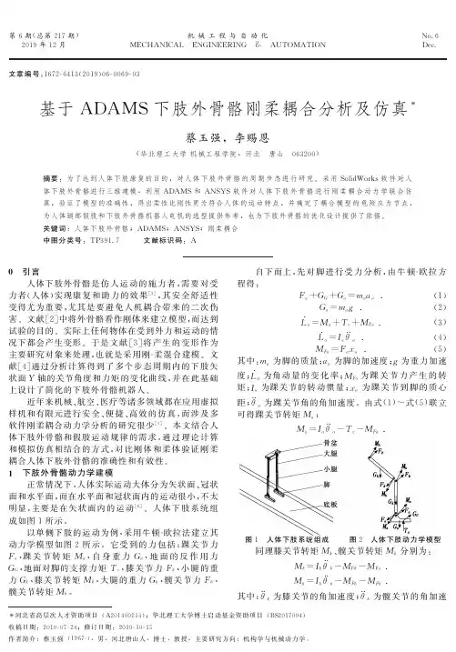
刚柔耦合仿真分析流程及要点
- 格式:doc
- 大小:160.50 KB
- 文档页数:4


机械系统中的刚柔耦合动力学分析引言机械系统的刚柔耦合动力学分析是研究刚性部件和柔性部件耦合工作时的振动特性和动力学性能的过程。
刚柔耦合系统由刚性和柔性部件组成,其刚性部件具有高刚度和低振动特性,柔性部件则具有低刚度和高振动特性。
刚柔耦合分析在现代工程设计和制造中具有重要的作用,尤其是在飞行器、机器人、精密仪器等领域中的应用。
一、刚柔耦合动力学模型刚柔耦合动力学模型是描述该系统振动行为的数学模型。
该模型可以基于刚体动力学和弹性体动力学原理建立。
刚体动力学模型涉及质点、刚体的平移和旋转运动方程,弹性体动力学模型涉及刚体振动的波动方程和柔性部件的变形方程。
综合考虑刚体和弹性体的动力学模型,可建立刚柔耦合动力学模型,用于研究振动响应和动力学性能。
二、刚柔耦合系统的耦合方式刚柔耦合系统的耦合方式主要包括刚体与柔性部件的物理耦合和动力学耦合。
物理耦合是指刚体和柔性部件通过连接件(如螺栓、焊接等)实现的实体耦合,确保其共同工作。
动力学耦合是指刚体和柔性部件在振动过程中相互作用和影响。
物理耦合和动力学耦合的研究有助于理解刚柔耦合系统的振动特性和动力学行为,提高系统工作的稳定性和可靠性。
三、刚柔耦合系统的振动特性分析刚柔耦合系统的振动特性是研究该系统固有频率、模态形状和振型等振动性质的过程。
通过振动特性分析,可以确定系统的谐振频率和振型,为系统优化设计和振动控制提供依据。
常用的方法包括有限元分析、模态分析和振动测试等。
其中,有限元分析是一种基于数值计算的方法,可以模拟系统的振动响应,模态分析可以获得系统的固有频率和模态形状,振动测试可以直接测量系统的振动状态。
四、刚柔耦合系统的动力学性能分析刚柔耦合系统的动力学性能是研究该系统在外部激励作用下的响应和行为。
动力学性能分析主要包括动力学模态分析、频率响应分析和阻尼特性分析等。
动力学模态分析可以研究系统在特定工况下的振动行为和能量分布,频率响应分析可以研究系统在不同频率下的响应特性,阻尼特性分析可以研究系统的振动耗能和稳定性。

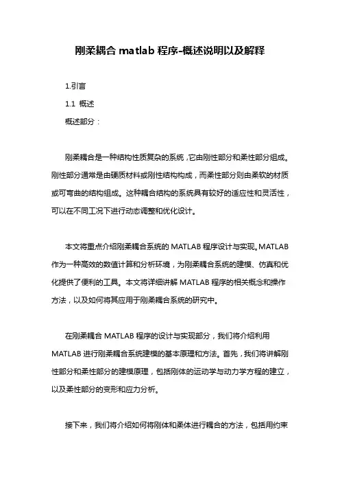
泵车臂架刚柔耦合模型仿真《机械工程与自动化杂志》2014年第二期1柔性体理论及创建方法多柔性体系统动力学是研究由可变形物体以及刚体所组成的系统在经历大范围空间运动时的动力学行为[3]。
它在多刚体动力学理论基础上,不仅考虑了各部件连接点处的阻尼与弹性等的影响,又进一步考虑到部件的变形,极大地提高了多体系统仿真的准确性。
1.1柔性体运动学方程在多柔性体系统动力学分析中,系统能量是一个非常重要的物理量。
同时,在理论计算过程中,能量的时间历程能否遵循保守系统能量守恒的原理保持常数,是考核计算结果正确与否的一个重要的指标。
柔性体的动能可表示为。
运用拉格朗日乘子法建立的多柔性体运动微分方程为:其中:K,M,D分别为模态刚度矩阵、质量矩阵和阻尼矩阵;Dξ•,Kξ分别为物体内部由于阻尼和弹性变形而引起的广义力;ψ为全局坐标基相对于局部坐标基的角度;λ为有约束的拉格朗日乘子;Q为外力作用下的广义力;fg为广义重力。
1.2柔性体创建方法使用ADAMS软件创建柔性体有3种方法[5]:①利用ADAMS中柔性梁的方法,即将模型中的某一个构件离散成许多段刚性单元,经过离散化的构件之间采用柔性梁的方式连接,然后为每一段离散件赋予不同的材料、颜色等属性,指定柔性梁的参数,但这种方法仅限于外形简单的构件时才能够使用,而且离散连接的实质并不是建立了真正意义上的柔性体,只是刚性体与刚性体的柔性连接;②利用ADAMS中的AutoFlex模块,在View模式下直接建立柔性体的模态中性文件,然后再利用该文件创建的柔性体代替原有刚性体实现柔性化处理,但自ADAMS软件07版本以后,软件已淡化了本身制作柔性体的功能;③先将刚性体模型导入到有限元软件中,将其离散成细小的网格后,计算有限元模型的模态,最后将计算结果保存为MNF 文件导入到ADAMS中建立柔性体。
通过计算构件的固有频率和对应的模态,按照模态理论,本文采用第3种方法建立柔性臂架,建立臂架系统刚柔耦合模型的流程见图1。
基于 Adams刚柔耦合仿真分析及应用【摘要】:剪式稳定架系统常用于汽车车身输送线,可实现车身的升降与运输。
其上框架布置2台电机,通过皮带带动下框架和吊具,实现升降。
在实际运行过程中,由于存在升降皮带安装轮安装相位偏差、皮带缠绕驱动轮运行过程旋转半径波动、皮带不等长等因素,造成下框架倾斜。
在升降过程中,由于运动不平衡,4根剪式稳定架可能产生较大的作用力,存在安全隐患。
因为采用多刚体系统计算会产生卡死现象,所以对剪式稳定架进行柔性化处理,从而得到刚柔耦合的多体系统,然后进行动力学仿真分析,预测剪式稳定架的受力情况,为产品设计和优化提供参考。
【关键词】:剪式稳定架;Adams;刚柔耦合;仿真分析引言1996年,ADAMS推出ADAMS Flex模块,实现了同时包含刚体和柔体的机构动力学分析。
ADAMS中的柔性体分为离散式和模态式2种:离散式柔性体是把一个刚体构件离散为几个小刚性构件,小刚体构件之间通过柔性梁连接,离散式柔性体的变形是柔性梁的变形,并不是小刚体构件的变形,这种柔性体可以模拟物体的非线性变形,但只适用于简单结构;模态式柔性体是由ADAMS Flex模块或外部有限元软件生成,能根据构件的实际结构进行复杂建模,这种柔性体采用的是模态叠加法来模拟物体变形,故仅适用于线性结构的受力分析。
1刚柔耦合基本理论在外部载荷作用下,物体一定会发生弹性变形,所以,多体系统都可以等效认为是一个多柔性系统。
在这种情况下,如果所研究的部件刚度大并且不考虑部件的应力-应变响应,则可以将该部件视为刚体。
但是当所研究部件的弹性变形对系统的影响较大,或者在外部载荷作用下部件的变形较为明显时,则必须考虑部件的弹性系数。
此时,就需要把所研究部件进行柔性化处理,以使多体系统更接近实际情况。
本文进行刚柔耦合仿真时采用了RecurDyn中提供的有限元柔性体建模。
有限元柔性体实现了有限元技术与多体动力学的有机结合,克服了模态柔性体对接触问题建模不准确,柔性体变形后模态需要及时更新的缺点,采用节点之间的相对位移和旋转作为节点坐标来描述结构的变形,具有较高的计算精度。

大范围运动刚柔耦合系统动力学建模与仿真随着科技的不断发展,机器人技术在各个领域得到了广泛的应用。
机器人的运动控制是机器人技术中的一个重要研究方向。
在机器人的运动控制中,刚柔耦合系统动力学建模与仿真是一个重要的研究方向。
刚柔耦合系统是指由刚体和柔性结构组成的系统。
刚体是指具有固定形状和大小的物体,而柔性结构则是指具有一定弹性的物体。
刚柔耦合系统的动力学建模与仿真是指对这种系统进行数学建模和仿真分析,以便更好地理解和控制这种系统的运动。
在刚柔耦合系统的动力学建模中,需要考虑刚体和柔性结构之间的相互作用。
这种相互作用可以通过建立刚柔耦合系统的动力学模型来描述。
动力学模型可以用来预测系统的运动轨迹和响应。
在建立动力学模型时,需要考虑系统的质量、惯性、弹性和摩擦等因素。
在刚柔耦合系统的仿真分析中,可以使用计算机模拟的方法来模拟系统的运动。
计算机模拟可以帮助研究人员更好地理解系统的运动特性,并预测系统的响应。
在进行仿真分析时,需要考虑系统的初始状态、外部扰动和控制策略等因素。
刚柔耦合系统的动力学建模与仿真在机器人技术中具有广泛的应用。
例如,在机器人的运动控制中,刚柔耦合系统的动力学建模和仿真可以帮助研究人员更好地理解机器人的运动特性,并设计更有效的控制策略。
此外,在机器人的设计和制造中,刚柔耦合系统的动力学建模和仿真也可以帮助研究人员更好地理解机器人的结构和性能,并优化机器人的设计。
刚柔耦合系统的动力学建模与仿真是机器人技术中的一个重要研究方向。
通过建立动力学模型和进行仿真分析,可以更好地理解和控制刚柔耦合系统的运动特性,从而为机器人技术的发展提供有力的支持。
第6期(总第169期)2011年12月机械工程与自动化MECHANICAL ENGINEERING & AUTOMATIONNo.6Dec.文章编号:1672-6413(2011)06-0071-03基于刚柔耦合的自动化动力学仿真分析研究张士存1,付月磊2(1.南车青岛四方机车车辆股份有限公司,山东 青岛 266111;2.安世亚太科技(北京)有限公司,北京 100026)摘要:刚柔耦合是多体系统最常见的力学模型,在其建模分析过程中存在一定的复杂性与重复性。
以三连杆机构为例,通过ANSYS和ADAMS实现刚柔耦合全分析过程,并利用ModelCenter的QuickWrap技术对整个分析过程的功能点进行组件封装,最后通过封装好的组件搭建刚柔耦合分析流程,最终实现自动化的刚柔耦合分析,为进一步的DOE及优化分析奠定了基础。
关键词:刚柔耦合;自动化;动力学;ANSYS;ADAMS中图分类号:TP391.9 文献标识码:A收稿日期:2011-06-28;修回日期:2011-07-08作者简介:张士存(1979-),男,山东济南人,工程师,本科,主要从事仿真集成及高性能计算集群应用工作。
0 引言在机械系统中,柔性体会对整个系统的运动产生重要影响,在进行运动学分析时如果不考虑柔性体的影响将会造成很大的误差,同样整个系统的运动情况也反过来决定了每个构件的受力状况和运动状态,从而决定了构件内部的应力应变分布。
因此采用ANSYS和ADAMS软件的联合仿真应运而生,它不但可以精确地模拟整个系统的运动,而且可以基于运动仿真的结果对运动系统中的柔性体进行应力应变分析[1,2]。
本文基于柔性体仿真的基本数学模型[3,4],以三连杆机构为例,进行刚柔耦合动力学仿真分析全过程研究。
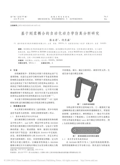
1 刚柔耦合分析本文所要分析的模型为三连杆机构,其中中间的连杆考虑作为柔性体,具体分析模型如图1所示。
1.1 柔性体模态中性文件生成进行刚柔耦合分析的第一步便是创建柔性体的模态中性文件*.mnf文件,模态中性文件是ADAMS软件进行刚柔耦合分析所需要的文件,它包含了柔性体的质量、质心、转动惯量、频率、振型以及对载荷的参与因子等信息,该步骤是在ANSYS中完成的。

刚柔耦合系统建模与仿真关键技术研究赵丽娟;马永志【摘要】研究了基于虚拟样机技术的复杂刚柔耦合多体系统建模与仿真中的关键技术,提出了保证仿真精度、缩短仿真时间,提高仿真速度的具体措施.大大提高了基于Pro/E、ANSYS和ADAMS三款软件联合进行刚柔耦合多体系统可靠性研究的操作性;解决了舍硫化铁矿结核体薄煤层采煤机截割部的输入实现、约束及边界条件等关键技术,为基于复杂煤层赋存条件下薄煤层采煤机截割部工作的可靠性研究提供了理论准备;找到了采煤机截割部关键零件设计上存在的问题,为采煤机截割部系统的优化提供了有力的量化依据:尤其是复杂刚-柔耦合多体系统建模与仿真中关键技术的解决对于研究多体系统工作的可靠性、降低研发成本、物理样机一次成功目标的实现具有重要的理论意义和较强的实用价值.【期刊名称】《计算机工程与应用》【年(卷),期】2010(046)002【总页数】6页(P243-248)【关键词】刚柔耦合;虚拟样机技术;机械系统动力学自动分析(ADAMS);模态中性文件(MNF)【作者】赵丽娟;马永志【作者单位】辽宁工程技术大学机械工程学院,辽宁,阜新,123000;辽宁工程技术大学机械工程学院,辽宁,阜新,123000【正文语种】中文【中图分类】TP391.9;TD421.6ZHAO Li-juan,MA Yong-zhi.Study on key technologies in modeling and simulation of rigid-flexible coupled multi-body puter Engineering and Applications,2010,46(2):243-248.由多个物体通过运动副连接的复杂机械系统称为多体系统,根据系统中物体的力学特性不同可分为刚性多体系统、柔性多体系统和刚柔耦合多体系统。
刚性多体系统是指可以忽略系统中物体的弹性变形而将其作为刚体来处理的系统,该类系统常处于低速运动状态;柔性多体系统是指系统在运动过程中会出现物体的大范围运动与物体的弹性变形的耦合,从而必须把物体当作柔性体处理的系统,大型、轻质、高速运动的机械系统常属此类;如果柔性多体系统中有部分物体可以当作刚体来处理,那么该系统就是刚柔耦合多体系统,这是多体系统中最普遍的模型[1]。
刚柔耦合matlab程序-概述说明以及解释1.引言1.1 概述概述部分:刚柔耦合是一种结构性质复杂的系统,它由刚性部分和柔性部分组成。
刚性部分通常是由硬质材料或刚性结构构成,而柔性部分则由柔软的材质或可弯曲的结构组成。
这种耦合结构的系统具有较好的适应性和灵活性,可以在不同工况下进行动态调整和优化设计。
本文将重点介绍刚柔耦合系统的MATLAB程序设计与实现。
MATLAB 作为一种高效的数值计算和分析环境,为刚柔耦合系统的建模、仿真和优化提供了便利的工具。
本文将详细讲解MATLAB程序的相关概念和操作方法,以及如何将其应用于刚柔耦合系统的研究中。
在刚柔耦合MATLAB程序的设计与实现部分,我们将介绍利用MATLAB进行刚柔耦合系统建模的基本原理和方法。
首先,我们将讲解刚性部分和柔性部分的建模原理,包括刚体的运动学与动力学方程的建立,以及柔性部分的变形和应力分析。
接下来,我们将介绍如何将刚体和柔体进行耦合的方法,包括用约束方程描述两者之间的关系和作用力的传递。
同时,我们还将介绍如何利用MATLAB的优化算法对刚柔耦合系统进行参数优化和动态调整,以使系统达到最佳的性能和效果。
最后,本文将总结刚柔耦合MATLAB程序的设计与实现过程,并阐述其在工程实际应用中的研究意义和潜在影响。
同时,我们还将展望未来刚柔耦合系统的发展方向和可能的研究方向。
通过本文的阅读,读者将能够了解刚柔耦合系统的概念及其与MATLAB程序的关系,掌握相关的建模和仿真方法,以及应用MATLAB 进行参数优化和动态调整的技巧。
希望本文能够为刚柔耦合系统的研究和应用提供一定的参考和指导。
1.2 文章结构文章结构部分将介绍本文的章节划分和各章节的主要内容。
本文共分为三个主要部分,分别是引言、正文和结论。
在引言部分(第一章),首先会对本文的研究主题刚柔耦合进行概述,解释刚柔耦合的概念和背景。
其次,将介绍本文的文章结构,给出每个章节的主要内容。
最后,明确本文的研究目的,即要设计和实现一个刚柔耦合MATLAB 程序。
1.In this lessonAfter completing this lesson, you will be able to:∙Create an SEMODES 103 – Flexible Body solution in Advanced Simulation. ∙Connect the flexible body finite element model to the degrees of freedom in the motion mechanism.∙Solve the finite element model and generate the RecurDyn Rflex input file.∙Define the flexible body in Motion Simulation and solve the motion mechanism.∙Animate the motion mechanism and observe the flexible body deformation.✓✓2. OverviewTypical motion simulations represent mechanisms using rigid bodies that move in prescribed degrees of freedom according to constraints. These rigid-body motion simulations cannot represent certain dynamic characteristics, especially those resulting from conditions such as sharp impacts, sudden changes in motion, or when the component is flexible enough to affect the motion of the mechanism. For these situations, you can use a flexible body analysis to combine both elastic deformation and rigid body motion.This type of analysis requires NX Motion Simulation with the RecurDyn solver and NX Advanced Simulation with the NX Nastran solver.T o set up a flexible body analysis for a component in your mechanism, you create a finite element model on the component and define stiffness at the points where it is connected to the mechanism (typically at joint locations). The NX Nastran SEMODES 103 – Flexible Body solution reduces the dynamic behavior of the flexible body to a set of mode shapes, which are stored in an output file. After you solve this modal solution, you associate the flexible body output file (.rfi file) with the link on which the component is defined in the motion simulation. When you solve the motion simulation, the RecurDyn solver communicates with NX Nastran and recovers the FE results. When you animate the mechanism, the contour plot for the flexible component is animated along with the rigid body animation.3. WorkflowAdvanced Simulation steps1.Create a finite element model and NX Nastran SEMODES 103 – FlexibleBody solution.2.Create a finite element mesh on the flexible component and assignmaterial properties.e a 1D Connection (spider element) or other constraint elements todefine the component's connection points to the mechanism.4.Add Fixed Boundary Degrees of Freedom constraints to defineconnection degrees of freedom.5.Add Free Boundary Degrees of Freedom constraints to define loaddegrees of freedom.6.Solve the modal solution. A RecurDyn Rflex input (.rfi) file is generatedfor the flexible link.7.Repeat steps 1–6 for each additional flexible component in themechanism.Motion Simulation steps1.Create a Flexible Body Dynamics motion simulation.2.Create flexible links on the flexible components. Associate each .rfi filewith each flexible link.3.Create a Flexible Body solution and add the flexible links to the solution.4.Solve the mechanism.5.Run Animation to view the combined rigid body and flexible body motion.6.Plot the modal degrees of freedom vs. time to determine the contributionof selected modes to the flexible body results.You can select one or more modes of the flexible body and then plot the modal displacement, acceleration, or velocity.4. Activity: Flexible body analysis — IntroductionEstimated time to complete: 12–16 minutesYou will learn how to:Define the flexible body in Motion Simulation and solve themotion mechanism.Animate the motion mechanism and observe the flexible bodydeformation.Note T o complete this activity, you must have the nx_motion_rflex license, in addition to Motion Simulation, Advanced Simulation, and NX Nastran.Launch the Flexible body analysis — Introduction activity.5. About the flexible body modal solutionYou will use the Advanced Simulation application to create a finite element model of the flexible body and perform a modal analysis. A modal analysis solves for the natural frequencies and mode shapes of flexible bodies.The NX Nastran SEMODES 103 – Flexible Body modal solution reduces the flexible body's mass and stiffness to modal space to represent its dynamic behavior. These reduced matrices are saved in the RecurDyn Rflex input file (.rfi).Then, in Motion Simulation, you associate the .rfi file with a link to create the flexible link.Example mode shapes6. About the finite element meshThe finite element model of a given body consists of a finite element mesh, material properties, and constraints.When you create a mesh on the body, the software divides the body into discrete regions called elements that are joined together at points called nodes. A group of elements is called a mesh.The mesh follows the shape of the body. When the model is solved, as the nodes in the mesh are displaced due to the analysis conditions such as loads, the behavior of each element is described by mathematical equations. The software finds the analysis solution by summing the individual element solutions.Example mesh of tetrahedral elementsIn Advanced Simulation, you create the mesh in the FEM file.When you use a smaller element size (resulting in more elements in a mesh), the accuracy of the solution is improved. However, as you refine the mesh, the solution time and computer resources needed to solve are also increased.7. Assigning a material to the meshIn Motion Simulation, material properties for a component are inherited from the master model on which you create the simulation. In Advanced Simulation, you must assign the same material to the flexible body finite element mesh as the material used for the flexible link in Motion Simulation.T o assign a material to the mesh, edit the mesh collector that contains the mesh. Then, modify the physical property table for the collector and open the Material List dialog box, where you can select the material to use.8. Connecting the flexible body FEM to the mechanismIn Advanced Simulation, in the FEM file, you must define the points where the flexible body is connected to the motion mechanism. These connection points must be defined at the origin point of every joint, bushing, force, torque, spring, or damper motion object on the flexible body.Although you can use any element type to define these connection points, typically you will use a 1D Connection (spider element).For accuracy in your flexible body solution, a single independent node (such as the core node of the spider element) in this connection element should be coincident with the motion object's origin point. You will define stiffness at this connection node using special constraints described in the next section.Spider elements defined at revolute joint locationsMake sure the connection node is at a location that creates balanced loading. For example, suppose you are connecting the flexible body to a revolute joint that is defined on a hole. Define the connection node in the bore center of the hole, rather than at the edge of the hole.Example of pinned connection (Revolute joint defined at bore center of hole)Connection node improperly defined at edge of holeConnection node properly defined at bore center of hole9. Defining connection and load degrees of freedom In Advanced Simulation, in the Simulation file, you must add special constraints to define the connection and load degrees of freedom for the flexible body.∙At each connection node where the flexible body will be connected to the mechanism through a joint or bushing in Motion Simulation, create a Fixed Boundary Degrees of Freedom constraint to define the connection degrees of freedom.∙At each connection node where a force, torque, spring, or damper will be applied to the flexible body in Motion Simulation, create a Free Boundary Degrees of Freedom constraint to define the load degrees of freedom.10. Solving the NX Nastran modal solutionIn the Solution dialog box for the SEMODES 103 – Flexible Body solution, you must specify the number of modes for which to solve and the result types to recover. By default, stress and displacement results are selected.After you have defined the finite element mesh, connection and load degrees of freedom, and solution attributes (such as the number of desired modes), you can solve the model.The solve produces several results files that you must not delete, move, or rename:∙.dat — Nastran input file, needed for later results recovery.∙.op2 — Contains the model geometry and component modes resulting from the modal analysis.∙_0.op2 — Needed for later results recovery; contains the component mode definitions, modal mass, and modal stiffness.∙.rfi — RecurDyn Rflex input file, needed for representing the flexible body in the RecurDyn solve.Remember the location of the .rfi file because you will need to point to it when creating the flexible link in Motion Simulation.11. ReviewQuestionIn the following example, suppose you are defining this excavator bucket asa flexible body in Advanced Simulation. In the motion mechanism, a single revolute joint is defined between the two holes (1 in the graphic below) at the top of the bucket. A force load is applied to one of the teeth (2).In Advanced Simulation, which constraints must you apply before solving the SEMODES 103 – Flexible Body solution? 2A Fixed Translation constraint and a Pinned constraintA Fixed Boundary Degrees of Freedom constraint and a Free Boundary Degrees of Freedom constraintA User Defined constraint and a Pinned constraintT wo Fixed constraintsAfter solving the SEMODES 103 – Flexible Body solution, when you create the flexible link in Motion Simulation, what file must you associate with the link to represent the dynamic behavior of the flexible body in themechanism?The .RFI fileThe .DAT file (Nastran input deck)The .OP2 fileThe .MDF file✓Show feedback12. Activity: Flexible body analysis — Advanced Simulation tasksEstimated time to complete: 12–16 minutesYou will learn how to:Create an SEMODES 103 – Flexible Body solution in AdvancedSimulation and specify a body as flexible.Connect the flexible body finite element model to the degreesof freedom in the motion mechanism.Solve the finite element model and generate the RecurDynRflex input file.Note T o complete this activity, you must have the nx_motion_rflex license, in addition to Motion Simulation, Advanced Simulation, and NX Nastran.Launch the Flexible body analysis — Advanced Simulation tasksactivity.13. Defining the flexible link in the mechanismIn Motion Simulation, you must create a Flexible Link that is associated with the component or body that you defined as flexible in Advanced Simulation.In the Flexible Link dialog box, you associate the link with the RecurDyn input file (.rfi file) generated by the NX Nastran modal solution. The Flexible Link Preview window helps you determine the correct method for positioning the flexible body on the link.In the graphics window, the flexible link is displayed with its finite element mesh.Meshed flexible link defined in the mechanism (and Preview view)14. Choosing modes to include in the analysisBy default, all modes from the NX Nastran modal solution are included in the motion simulation solve except the first six modes, which are consideredrigid-body modes.Including all modes ensures a more accurate representation of the structure. However, for better solve performance, you can reduce the modal model by removing insignificant modes.T o determine which modes to remove, you can view and animate the mode shapes using the Post Processing Navigator and Post Processing toolbar. Make sure to include all modes that resemble the behavior you are analyzing.Example mode shape✓✓15. Solving the model and animating the mechanismIn Motion Simulation, you create a Kinematics/Dynamics solution of type Flexible Body.When you solve the Flexible Body solution, the RecurDyn solver calculates the physical deformations at each point where the flexible body is connected to the rest of the mechanism, for each configuration of the motion mechanism. It saves these deformations in a modal deformation file (.mdf).Using the .mdf file, the motion solution process calls the NX Nastran solver to recover the deformation, displacement, stress, and other results on the original, unreduced flexible body. These transient results are then returned to Motion Simulation, where you can view them in an animation of the mechanism.By default, when you animate a flexible body solution, translational deformation results (nodal displacements) are displayed for the flexible body. You can also display other results, such as Displacement – Nodal, Stress – Element – Nodal and Strain – Element – Nodal, depending on the results you requested in the output request for the SEMODES 103 – Flexible Body solution in Advanced Simulation.16. Activity: Flexible body analysis — Motion Simulation tasksEstimated time to complete: 12–16 minutesYou will learn how to:Define the flexible body in Motion Simulation and solve themotion mechanism.Animate the motion mechanism and observe the flexible bodydeformation and stress.Run an interference check between the flexible link and a bodypanel.Note T o complete this activity, you must have the nx_motion_rflex license, in addition to Motion Simulation, Advanced Simulation, and NX Nastran.Launch the Flexible body analysis — Motion Simulation tasksactivity.Flexible body analysis — Introduction1. Open the Motion SimulationOpen (Standard toolbar)∙∙∙∙OK∙The motion simulation opens in the Motion Simulation application.2. Reset the dialog box settingsThe options you select in NX dialog boxes are preserved for the next time you open the same dialog box within an NX session. To ensure that the dialog boxes are in the expected initial state for each step-by-step activity, you should restore the default settings.Preferences→User Interface∙Reset Dialog Box Settings∙OK3. Enable the Flexible Body Dynamics environment The Flexible Body Dynamics environment is available only with the Dynamics analysis type.Environment (Motion toolbar)∙Flexible Body Dynamics∙OK✓✓4. Define the flexible linkFlexible Link (Motion toolbar)∙∙Flexible Model∙Browse∙intro_flex_body/fbcam_assy_sim2-solution_1_0.rfiThis pre-generated file contains a modal reduction of the flexible body's mass and stiffness, which represen ts the body’s dynamic behavior. The NX Nastran solver generates these reduced matrices and saves them in a RecurDyn Rflex input (RFI) file. In a later activity, you will solve an NX Nastran solution and generate an RFI file.∙OK RFI File dialog boxLeave the Flexible Link dialog box open for the next step.5. Finish defining the flexible linkThe Flexible Link dialog box is still open from the previous step.∙The Flexible Link Preview window shows you the meshed flexible body and its orientation relative to the absolute coordinate system.∙∙Because the flexible body is in the same orientation relative to the absolute coordinate system as the corresponding link in the mechanism, Absolute Origin is the appropriate selection.∙OK Flexible Link dialog box6. Create a Flexible Body solutionMotion Navigator∙motion_1∙New Solution∙∙∙∙∙OK7. Add the flexible link to the solutionMotion Navigator∙Flexible Links∙L002–fbcam_assy_sim2-solution_1∙Add to Solution8. Solve the motion simulationMotion Navigator∙Load Container∙G002∙Add to SolutionFor illustration purposes, this vector force simulates a load on the clevis in the X direction, to exaggerate the flexible behavior.∙Solution_2∙SolveThe solve process may take several minutes to complete. After the RecurDyn solve finishes, NX Nastran is called automatically to run the SEMODES 103 –Flexible Body solve. Nastran uses the RecurDyn results file and the original NX Nastran input file to recover the deformation, displacement, stress and other results for the flexible link.Caution Do NOT close any solve windows until all NX Nastran command prompt windows have closed and the message ―Nastran resultsrecovery completed‖ appears in the NX status line.9. Animate the mechanismAnimation (Motion toolbar, Simulation Drop-down list)∙Play(此处为动图,有需要可联系上传者)By default, the contour plot of the flexible link displays nodal translational deformation results. You can also display other results, such as Displacement – Nodal and Stress – Element – Nodal, depending on the results yourequested in the output request for the SEMODES 103 – Flexible Body solution in Advanced Simulation.∙OKYou completed the activity.Flexible body analysis — Advanced Simulation tasks1. Open the simulationOpen (Standard toolbar)∙∙∙∙OK∙The motion simulation opens in the Motion Simulation application.2. Reset the dialog box settingsThe options you select in NX dialog boxes are preserved for the next time you open the same dialog box within an NX session. To ensure that the dialog boxes are in the expected initial state for each step-by-step activity, you should restore the default settings.Preferences→User Interface∙Reset Dialog Box Settings∙OK3. Solve and animate the solutionBefore adding the flexible body, solve and animate the included solution to see the rigid-body motion of the mechanism.Motion Navigator∙Solution_1∙SolveAnimation (Motion toolbar, Simulation Drop-down list)Packaging Options∙Interference∙Pause on Event∙An Interference packaging option has been predefined between the suspension arm and the sheet body panel. When you animate the mechanism, if the suspension arm and body panel come into contact, the interferingbodies will be highlighted and the animation will pause.∙PlayAs you can see, no interference occurs. Later in this activity, we will check for interference again with the suspension arm defined as a flexible link.∙OK4. Start Advanced SimulationMotion Navigator∙_demo_assy∙Make WorkThis command changes the work part from the motion simulation to the part file.No Save Simulation Part File messageStart→Advanced Simulation5. Create Simulation and FEM filesSimulation Navigator∙_demo_assy.prt∙New FEM and SimulationThe New FEM and Simulation dialog box lists the three new files that will be created: the Simulation, FEM, and idealized part file.The Solver Environment section lists NX Nastran as the solver. The Analysis Type is Structural.∙∙(the lower suspension arm)∙OK New FEM and Simulation dialog box∙The Solution dialog box appears.∙∙Case Control∙Edit (Lanczos Data)∙∙∙This specified frequency range means the solver will calculate the lowest-frequency modes within the first 20 modes starting from thefrequency of 0.∙If you increase the number of desired modes, you can achieve a more accurate representation of the structure, but at the expense of solution time.You should include enough modes to cover the frequency range of interest (based on your particular mechanical system).∙OK Real Eigenvalue – Lanczos dialog boxCaution Accept the default settings for Flexible Body Solution Type and Flexible Body Export Options. These options are intended formanual integration with RecurDyn or Adams software packages, andshould not be changed for NX Motion Simulation. If you change thesedefault settings, the Motion Simulation flexible body solution maynot solve.∙OK Solution dialog box∙6. Connect the flexible body FEM to the mechanism You must define the points where the flexible body is connected to other degrees of freedom in the motion mechanism. Although you can use any elementtype to connect the flexible body, typically you will use a 1D Connection (spider element).Simulation Navigator∙Simulation File ViewNote If the Simulation File View is not visible, click thebar at the bottom of the Simulation Navigator to open it.∙_demo_assy_fem1The FEM file is displayed in the graphics window, and is listed at the top of the Simulation Navigator.Static Wireframe (View toolbar, Rendering Style Drop-down list)1D Connection (Advanced Simulation toolbar, ConnectionsDrop-down list)∙∙(Select Point)∙∙Arc/Ellipse/Sphere Center (Specify Point 1 and Specify Point 2)∙,Note Select the arc centers of the top and bottom edges.∙OK Point dialog box∙(the face)∙Connection Element∙∙Apply∙∙This creates a connection recipe. In a later step in this activity, when you create a solid mesh on the part, the connection recipe will generate a spider element using nodes defined in the geometry mesh.∙Repeat the above steps to create Point to Face RBE2 connection recipes on the other two ends of the arm, as shown in the following pictures.When you are finished, close the 1D Connection dialog box.7.Mesh the partNow create a tetrahedral mesh on the solid body.Shaded with Edges (View toolbar, Rendering Style Drop-down list)3D Tetrahedral Mesh (Advanced Simulation toolbar, MeshDrop-downlist)∙the part∙∙Mesh Parameters∙∙in the regions where bending is predicted. At least three layers of solidelements are needed to accurately model bending.∙OK∙∙The part is meshed with tetrahedral solid elements and the connection recipes are now 1D spider elements.∙8. Create a node groupLater in this activity, you will need to define stiffness at the node at the center of each of the three 1D connections you created previously. To make that step easier, you will add these nodes to a node group.Simulation Navigator∙Groups∙New Group∙Node Labels∙Because you created the connection recipes before you meshed the part, the core nodes of the resulting 1D connections are labeled 1, 2, and 3. You will add these nodes to the group by entering their labels.∙∙Select∙∙OK9. Define material propertiesSimulation Navigator∙3D Collectors (expand)∙Solid(1)∙Edit∙Edit (Solid Property)∙Properties∙Choose material∙∙OK all dialog boxes10. Display the Simulation fileSimulation Navigator∙Simulation File View∙_demo_assy_sim111. Define connection degrees of freedomIn a previous step, you created spider elements at the three ends of the suspension arm. The independent node at the center of each spider element was defined to be coincident with the origin point of a joint or bushing that connects this component to the mechanism. You will now define the local stiffness at these connection points using a Fixed Boundary Degrees of Freedom constraint.Static Wireframe (View toolbar, Rendering Style Drop-down list)Fixed Boundary Degrees of Freedom (Advanced Simulation toolbar,Constraint Type list )∙Model Objects∙Group Reference∙_demo_assy_fem2::connection_nodesNote This is the node group you created in the previous step.∙Degrees of Freedom∙All OnT o ensure the correct local stiffness at the connection points, always set all DOF to On when creating Fixed Boundary Degrees of Freedom or Free Boundary Degrees of Freedom constraints in a flexible body analysis.∙OK∙∙When you created the connection recipe for each spider element, you placed the independent node at the bore center of the hole rather than at the arc center of the edge of the hole. This placement ensures balanced loading.Save (Standard toolbar)12. Solve the modelYou will solve the model to generate the .rfi file that contains the reduced matrices that represent the component's dynamic behavior. This file will be used later in the activity when you solve the Flexible Body solution in Motion Simulation.Simulation Navigator (main view)∙Solution 1∙Solve∙OK∙Y ou can ignore the Information window warning concerning rigid links.∙The Analysis Job Monitor dialog box appears.∙Wait for the job to finish and for the command window to close. This process may take several minutes.∙Close Solution Monitor dialog box∙Cancel Analysis Job Monitor dialog box∙Information window∙Solution 1∙BrowseIn the explorer window that opens, note the location of the .rfi file. It should be located in the f1_car_flex_body folder, and should be named similar to_demo_assy_sim1-solution_1_0.rfi.13. View the mode shapesSimulation Navigator∙ResultsPost Processing Navigator∙Solution 1 (expand)The first six modes are rigid body modes.∙Mode 7 (expand)∙Displacement – Nodal (expand)∙MagnitudeNote The ends of the part overlap because of the default deformation scale, which is set to 10% of the model. You can reduce the scaling using EditPost View(Post-Processing toolbar).Next Mode/Iteration (Post Processing toolbar)Use the Next Mode/Iteration command to view additional modes.Return to Model (Layout Manager toolbar)Save (Standard toolbar)In a later activity, you will connect the flexible body to a motion mechanism. If you plan to complete the next Flexible Body activity, leave this simulation file open in NX.You completed the activity.Flexible body analysis — Motion Simulation tasks1. Open the Motion SimulationIf you completed the steps in the previous Flexible Body activity and your_demo_assy_sim1.sim part is still open in NX, use these steps.If the part is not still open, or if you did not complete the previous Flexible Body activity, skip to the next page.Simulation Navigator∙Simulation File View∙_demo_assy∙Make Displayed PartThis command changes the work part from the simulation file to the master model assembly.Start→Motion SimulationMotion Navigator∙motion_1Skip the next page and move on to page 3.2. Open the Motion SimulationUse these steps if the _demo_assy_sim1.sim part was not still open from the previous Flexible Body activity.Open (Standard toolbar)∙∙∙∙OK∙The motion simulation opens in the Motion Simulation application.3. Reset the dialog box settingsThe options you select in NX dialog boxes are preserved for the next time you open the same dialog box within an NX session. To ensure that the dialog boxes are in the expected initial state for each step-by-step activity, you should restore the default settings.Preferences→User Interface∙Reset Dialog Box Settings∙OK4. Enable the Flexible Body Dynamics environmentThe Flexible Body Dynamics environment is available only with the Dynamics analysis type.Environment (Motion toolbar)∙Flexible Body Dynamics∙OK5. Define the flexible linkFlexible Link (Motion toolbar)∙Note You can select any part of the indicated link.∙Flexible Model∙Browse∙_demo_assy_sim1–solution_1_0.rfiThis is the .rfi file generated from the NX Nastran solve in the previous Flexible Body activity. It should be located in the f1_car_flex_body folder along with the FEM and Simulation files you created in Advanced Simulation.Note If you did not complete the previous Flexible Body activity, copy the provided Simulation file, named _demo_assy_sim1.sim, from the。
一、引言航空发动机作为飞机的动力来源,在飞行过程中扮演着至关重要的角色。
其质量、性能和可靠性对飞机的整体性能有着巨大的影响。
为了提高航空发动机的性能和可靠性,研究人员需要对其运动机构进行深入的研究和仿真分析。
高精度的动力学仿真方法可以帮助研究人员更好地理解航空发动机的运动特性,为发动机设计和改进提供重要参考。
二、航空发动机运动机构高精度动力学仿真的重要性1. 航空发动机运动机构的复杂性航空发动机是由众多部件组成的复杂系统,其运动机构包含了众多的刚体和弹性部件,涉及到多种不同的力学和动力学问题。
针对这些复杂性,传统的动力学仿真方法往往难以对航空发动机的运动特性进行准确的模拟和分析。
2. 动力学仿真精度的要求航空发动机在高速旋转和高温高压环境下工作,其运动机构的精度要求极高。
动力学仿真方法需要能够准确地描绘航空发动机在不同工况下的运动特性,以满足对精度的要求。
三、航空发动机运动机构高精度刚柔耦合动力学仿真的研究现状目前,针对航空发动机运动机构的高精度动力学仿真方法的研究主要集中在以下几个方面:1. 刚体动力学仿真研究人员通过建立刚体系统的数学模型,利用动力学理论分析航空发动机在运转过程中的姿态、速度和加速度等运动特性。
2. 弹性动力学仿真考虑到航空发动机在高速旋转时的弹性变形特性,研究人员开展了针对弹性部件的动力学仿真研究,以描绘发动机在工作过程中的弹性振动和应力分布等特性。
3. 刚柔耦合动力学仿真近年来,越来越多的研究人员开始关注航空发动机运动机构中刚体和弹性部件的耦合效应,开展了刚柔耦合动力学仿真的研究工作。
这些研究致力于描绘刚体和弹性部件之间的相互作用和影响,以提高动力学仿真的精度。
四、航空发动机运动机构高精度刚柔耦合动力学仿真方法的研究进展1. 建立高精度的数学模型针对航空发动机的复杂运动机构,研究人员需要建立高精度的数学模型,描述刚体和弹性部件之间的相互作用和影响。
通过精确的数学模型,可以更准确地描绘航空发动机在不同工况下的运动特性。
本文主要介绍使用SolidWorks、HyperMesh、ANSYS和ADAMS软件进行刚柔耦合动力学分析的主要步骤。
一、几何建模
在SolidWorks中建立几何模型,将模型调整到合适的姿态,保存。
此模型的姿态不要改动,否则以后的MNF文件导入到ADAMS中装配起来麻烦。
二、ADAMS动力学仿真分析
将模型导入到ADAMS中进行动力学仿真分析。
为了方便三维模型的建立,SolidWorks中是将每个零件单独进行建模然后在装配模块中进行装配。
这一特点导致三维模型导入到ADAMS软件后,每一个零件都是一个独立的part,由于工作装置三维模型比较复杂,因此part数目也就相应的比较多,这样就对仿真分析的进行产生不利影响。
下面总结一下从三维建模软件SolidWorks导入到ADAMS中进行机构动力学仿真的要点。
(1)首先在SolidWorks中得到装配体。
(2)分析该装配体中,到底有几个构件。
(3)分别隐藏其他构件而只保留一个构件,并把该构件导出为*.x_t 格式文件。
(4)在ADAMS中依次导入各个*.x_t 文件,并注意是用part的形式导入的。
(5)对各个构件重命名,并给定颜色,设置其质量属性。
(6)对于产生相对运动的地方,建议先在此处创建一个marker,以方便后面的操作。
否则,三维模型进入ADAMS后,线条繁多,在创建运动副的时候很难找到对应的点。
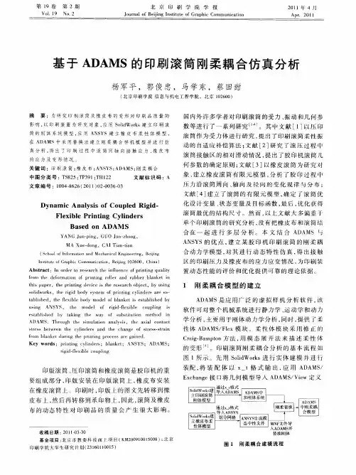
部件的导入如下图1所示:
图1 文件输入
File Type选择Parasolid;
File To Read 找到相应的模型;
将Model Name 切换到Part Name,然后在输入框中右击,一次单击part →create 然后在弹出的新窗口中设置相应的Part Name,然后单击OK →OK 。
将一个部件导入,重复以上步骤将部件依次导入。
这里输入的技巧是将部件名称按顺序排列,如zpt_1、zpt_2、zpt_3. ,然后在图1中只需将zpt_1改为zpt_2、将PART_1改为PART_2即可。
三、HyperMesh中创建柔性体部件的有限元模型。
在SolidWorks中把其他部件隐藏,只显示将要柔性化的部件,模型另存为.iges 格式,导入到HyperMesh中进行前处理。
或者将整个模型都导入到HyperMesh中,但只创建需要柔性化的部件有限元模型。
(1) 选择单元类型,赋予材料属性:实体采用Solid185单元类型,壳单元采用shell181单元类型(其他亦可,根据需要选择)。
然后创建材料,赋予属性。
(2)单位的统一:因为在SolidWorks中建模一般使用的长度单位是mm,而ADAMS中使用mm的单位系统只有mm、 Kg、N、s、deg。
因此,通过换算和推导,在HyperMesh (ANSYS)中使用的单位为:mm、Kg、s、e-3N、e3Pa。
例如,钢材的弹性模量为2.1e8(e3Pa)、密度7.85e-6(Kg/mm3)、泊松比0.3。
(3)外部节点的设置:在柔性体与刚性体的铰接处必须有节点存在才能实现铰接,在ADAMS中将其作为外部节点使用,从模型的装配与约束方面考虑,一个铰接点只需要设置一个节点作为外部节点。
外部节点的生成选用mass21质量点加上刚性区域法(刚性蜘蛛网),如图2 所示。
图2 外部节点
四、MNF(模态中性文件)的生成
在HyperMesh中完成所有的前处理工作后,导出为ANSYS可读取的后缀为.cbd的文件。
然后打开ANSYS软件,读取该文件。
点击操作界面Main Menu-Solution - Adams Connection-Export to ADAMS,弹出reselect attachment nodes对话框,选取外部节点作为外连接点,有几个选几个。
然后弹出Export to ADAMS 对话框,在这一步中需要注意的是单位系统,在ADAMS与ANSYS中的单位系统需要保持一致。
选择自定义单位系统,打开
Define User Unit 对话框,设置Length Factor为1000,Force Factor为1000,如图3所示。
另外,根据实际需要在ANSYS中选择生成的模态的阶数。
Element Results 选择Include Stress and Strain,然后单击Solve and create export file to ADAMS,生成.MNF文件。
图3 Export to ADAMS
五、刚柔替换
将模态中性文件.MNF 导入ADAMS,替换掉刚性的部件,得到刚柔耦合模型。
由于采用替换刚性体的方法,导致原刚性体和柔性体的marker点发生变化,因此必须对边界条件重新审视,建议删除该柔性体上的全部边界条件,重新对柔性体施加约束,以防出错。
可通过以下途径来检查柔性体正确与否:检查质量、质心位置、惯性矩;比较ANSYS中模态分析结果与ADMAS中柔性体的模态和振型;比较最大静力变形量/应力值是否与有限元模型相同。
刚柔耦合替换步骤:在模型树上选择需要替换的刚性部件,然后右击选择Make Flexible,弹出Make Flexible 对话框,选择IMPORT MNF ,弹出Swap a rigid body for a flexible body 对话框,在MNF File 中选择对应的.MNF文件,点击OK按钮。
如图4所示
图4 刚柔替换
六、刚柔耦合动力学仿真分析
然后就可以进行刚柔耦合动力学仿真分析了。
根据计算机性能和实际仿真的需要,可以把多个部件设置成柔性体,也可以全部设为柔性体。