OTSU算法matlab程序代码

标题：探索MATLAB中各类拟合曲线的代码应用在MATLAB中，拟合曲线是数据分析和模型建立中常用的技术之一。

通过拟合曲线，我们可以了解数据之间的关联性并建立预测模型，为进一步分析和应用数据奠定基础。

本文将深入探讨MATLAB中各类拟合曲线的代码应用，帮助读者更深入地理解该主题。

一、线性拟合曲线1. 使用MATLAB进行线性拟合曲线的代码示例在MATLAB中，使用polyfit函数可以进行线性拟合。

对一组数据点(x, y)进行线性拟合，代码如下：```matlabx = [1, 2, 3, 4, 5];y = [2, 3.5, 5, 7, 8.5];p = polyfit(x, y, 1);```其中，x为自变量，y为因变量，1表示进行一次线性拟合。

通过polyfit函数，可以得到线性拟合的系数p。

2. 线性拟合曲线的应用和特点线性拟合曲线适用于线性关系较为明显的数据，例如物理实验数据中的直线关系。

通过线性拟合，可以获得各项系数，对数据进行预测和建模。

二、多项式拟合曲线1. 使用MATLAB进行多项式拟合曲线的代码示例在MATLAB中，使用polyfit函数同样可以进行多项式拟合。

对一组数据点(x, y)进行二次多项式拟合，代码如下：```matlabx = [1, 2, 3, 4, 5];y = [1, 4, 9, 16, 25];p = polyfit(x, y, 2);```其中，x为自变量，y为因变量，2表示进行二次多项式拟合。

通过polyfit函数，同样可以得到多项式拟合的系数p。

2. 多项式拟合曲线的应用和特点多项式拟合曲线适用于数据中存在曲线关系的情况，通过选择合适的最高次数，可以灵活地拟合各种曲线形状。

三、非线性拟合曲线1. 使用MATLAB进行非线性拟合曲线的代码示例在MATLAB中，使用fit函数可以进行非线性拟合。

对一组数据点(x, y)进行指数函数拟合，代码如下：```matlabx = [1, 2, 3, 4, 5];y = [2.1, 7.4, 16.1, 29.3, 48.2];f = fit(x', y', 'exp1');```其中，x为自变量，y为因变量，'exp1'表示进行指数函数拟合。

专业综合课程设计任务书学生姓名: 专业班级: 电信指导教师: 周颖工作单位: 信息工程学院题目:图像OTSU阈值分割的程序设计初始条件:（1）提供实验室机房及其matlab软件；（2）数字图像处理的基本理论学习。

要求完成的主要任务:(包括课程设计工作量及其技术要求,以及说明书撰写等具体要求):（1）掌握数字图像分割的基本原理；（2）选择一幅256级的灰度图像，利用matlab设计程序完成以下功能；（3）根据OTSU（最大类间方差法）原理，设计求取阈值的程序（不能使用matlab 的库函数），并与用matlab的库函数求得的阈值进行比较；（4）用求得的阈值对一灰度图片进行分割，并对结果进行分析；（5）要求阅读相关参考文献不少于5篇；（6）根据课程设计有关规范，按时、独立完成课程设计说明书。

时间安排:(1) 布置课程设计任务，查阅资料，确定方案 1.5天；(2) 进行编程设计、调试2天；(3) 完成课程设计报告书、答辩 1.5天；指导教师签名: 年月日系主任(或责任教师)签名: 年月日目录1概述 (1)2 MATLAB常用图像操作函数 (2)2.1图像的读写 (2)2.2图像的显示 (2)3理论知识 (3)3.1图像分割的定义 (3)3.2阈值分割 (4)3.3最大类间方差法(OTSU) (4)3.4全局阈值 (5)4实验程序 (6)5程序运行结果及分析 (9)5.1程序运行结果 (9)5.2结果分析 (14)6心得体会 (15)参考文献 (16)1概述数字图像处理(DigitalImageProcessing)是通过计算机对图像进行去除噪声、增强、复原、分割、提取特征等处理的方法和技术。

数字图像处理的产生和迅速发展主要受三个因素的影响:一是计算机的发展;二是数学的发展(特别是离散数学理论的创立和完善);三是广泛的农牧业、林业、环境、军事、工业和医学等方面的应用需求的增长。

数字图像处理研究的内容主要有:(1)图像获取和图像表现阶段主要是把模拟图像信号转化为计算机所能接受的数字形式,以及把数字图像用所需要的形式显示出来。

30个智能算法matlab代码以下是30个使用MATLAB编写的智能算法的示例代码： 1. 线性回归算法：matlab.x = [1, 2, 3, 4, 5];y = [2, 4, 6, 8, 10];coefficients = polyfit(x, y, 1);predicted_y = polyval(coefficients, x);2. 逻辑回归算法：matlab.x = [1, 2, 3, 4, 5];y = [0, 0, 1, 1, 1];model = fitglm(x, y, 'Distribution', 'binomial'); predicted_y = predict(model, x);3. 支持向量机算法：matlab.x = [1, 2, 3, 4, 5; 1, 2, 2, 3, 3];y = [1, 1, -1, -1, -1];model = fitcsvm(x', y');predicted_y = predict(model, x');4. 决策树算法：matlab.x = [1, 2, 3, 4, 5; 1, 2, 2, 3, 3]; y = [0, 0, 1, 1, 1];model = fitctree(x', y');predicted_y = predict(model, x');5. 随机森林算法：matlab.x = [1, 2, 3, 4, 5; 1, 2, 2, 3, 3]; y = [0, 0, 1, 1, 1];model = TreeBagger(50, x', y');predicted_y = predict(model, x');6. K均值聚类算法：matlab.x = [1, 2, 3, 10, 11, 12]; y = [1, 2, 3, 10, 11, 12]; data = [x', y'];idx = kmeans(data, 2);7. DBSCAN聚类算法：matlab.x = [1, 2, 3, 10, 11, 12]; y = [1, 2, 3, 10, 11, 12]; data = [x', y'];epsilon = 2;minPts = 2;[idx, corePoints] = dbscan(data, epsilon, minPts);8. 神经网络算法：matlab.x = [1, 2, 3, 4, 5];y = [0, 0, 1, 1, 1];net = feedforwardnet(10);net = train(net, x', y');predicted_y = net(x');9. 遗传算法：matlab.fitnessFunction = @(x) x^2 4x + 4;nvars = 1;lb = 0;ub = 5;options = gaoptimset('PlotFcns', @gaplotbestf);[x, fval] = ga(fitnessFunction, nvars, [], [], [], [], lb, ub, [], options);10. 粒子群优化算法：matlab.fitnessFunction = @(x) x^2 4x + 4;nvars = 1;lb = 0;ub = 5;options = optimoptions('particleswarm', 'PlotFcn',@pswplotbestf);[x, fval] = particleswarm(fitnessFunction, nvars, lb, ub, options);11. 蚁群算法：matlab.distanceMatrix = [0, 2, 3; 2, 0, 4; 3, 4, 0];pheromoneMatrix = ones(3, 3);alpha = 1;beta = 1;iterations = 10;bestPath = antColonyOptimization(distanceMatrix, pheromoneMatrix, alpha, beta, iterations);12. 粒子群-蚁群混合算法：matlab.distanceMatrix = [0, 2, 3; 2, 0, 4; 3, 4, 0];pheromoneMatrix = ones(3, 3);alpha = 1;beta = 1;iterations = 10;bestPath = particleAntHybrid(distanceMatrix, pheromoneMatrix, alpha, beta, iterations);13. 遗传算法-粒子群混合算法：matlab.fitnessFunction = @(x) x^2 4x + 4;nvars = 1;lb = 0;ub = 5;gaOptions = gaoptimset('PlotFcns', @gaplotbestf);psOptions = optimoptions('particleswarm', 'PlotFcn',@pswplotbestf);[x, fval] = gaParticleHybrid(fitnessFunction, nvars, lb, ub, gaOptions, psOptions);14. K近邻算法：matlab.x = [1, 2, 3, 4, 5; 1, 2, 2, 3, 3]; y = [0, 0, 1, 1, 1];model = fitcknn(x', y');predicted_y = predict(model, x');15. 朴素贝叶斯算法：matlab.x = [1, 2, 3, 4, 5; 1, 2, 2, 3, 3]; y = [0, 0, 1, 1, 1];model = fitcnb(x', y');predicted_y = predict(model, x');16. AdaBoost算法：matlab.x = [1, 2, 3, 4, 5; 1, 2, 2, 3, 3];y = [0, 0, 1, 1, 1];model = fitensemble(x', y', 'AdaBoostM1', 100, 'Tree'); predicted_y = predict(model, x');17. 高斯混合模型算法：matlab.x = [1, 2, 3, 4, 5]';y = [0, 0, 1, 1, 1]';data = [x, y];model = fitgmdist(data, 2);idx = cluster(model, data);18. 主成分分析算法：matlab.x = [1, 2, 3, 4, 5; 1, 2, 2, 3, 3]; coefficients = pca(x');transformed_x = x' coefficients;19. 独立成分分析算法：matlab.x = [1, 2, 3, 4, 5; 1, 2, 2, 3, 3]; coefficients = fastica(x');transformed_x = x' coefficients;20. 模糊C均值聚类算法：matlab.x = [1, 2, 3, 4, 5; 1, 2, 2, 3, 3]; options = [2, 100, 1e-5, 0];[centers, U] = fcm(x', 2, options);21. 遗传规划算法：matlab.fitnessFunction = @(x) x^2 4x + 4; nvars = 1;lb = 0;ub = 5;options = optimoptions('ga', 'PlotFcn', @gaplotbestf);[x, fval] = ga(fitnessFunction, nvars, [], [], [], [], lb, ub, [], options);22. 线性规划算法：matlab.f = [-5; -4];A = [1, 2; 3, 1];b = [8; 6];lb = [0; 0];ub = [];[x, fval] = linprog(f, A, b, [], [], lb, ub);23. 整数规划算法：matlab.f = [-5; -4];A = [1, 2; 3, 1];b = [8; 6];intcon = [1, 2];[x, fval] = intlinprog(f, intcon, A, b);24. 图像分割算法：matlab.image = imread('image.jpg');grayImage = rgb2gray(image);binaryImage = imbinarize(grayImage);segmented = medfilt2(binaryImage);25. 文本分类算法：matlab.documents = ["This is a document.", "Another document.", "Yet another document."];labels = categorical(["Class 1", "Class 2", "Class 1"]);model = trainTextClassifier(documents, labels);newDocuments = ["A new document.", "Another new document."];predictedLabels = classifyText(model, newDocuments);26. 图像识别算法：matlab.image = imread('image.jpg');features = extractFeatures(image);model = trainImageClassifier(features, labels);newImage = imread('new_image.jpg');newFeatures = extractFeatures(newImage);predictedLabel = classifyImage(model, newFeatures);27. 时间序列预测算法：matlab.data = [1, 2, 3, 4, 5];model = arima(2, 1, 1);model = estimate(model, data);forecastedData = forecast(model, 5);28. 关联规则挖掘算法：matlab.data = readtable('data.csv');rules = associationRules(data, 'Support', 0.1);29. 增强学习算法：matlab.environment = rlPredefinedEnv('Pendulum');agent = rlDDPGAgent(environment);train(agent);30. 马尔可夫决策过程算法：matlab.states = [1, 2, 3];actions = [1, 2];transitionMatrix = [0.8, 0.1, 0.1; 0.2, 0.6, 0.2; 0.3, 0.3, 0.4];rewardMatrix = [1, 0, -1; -1, 1, 0; 0, -1, 1];policy = mdpPolicyIteration(transitionMatrix, rewardMatrix);以上是30个使用MATLAB编写的智能算法的示例代码，每个算法都可以根据具体的问题和数据进行相应的调整和优化。

《数字图像处理实验报告》实验一图像的增强一.实验目的1.熟悉图像在MATLAB下的读写、输出；2.熟悉直方图；3.熟悉图像的线性指数等；4.熟悉图像的算术运算和几何变换。

二.实验仪器计算机、MATLAB软件三.实验原理图像增强是指根据特定的需要突出图像中的重要信息，同时减弱或去除不需要的信息。

从不同的途径获取的图像，通过进行适当的增强处理，可以将原本模糊不清甚至根本无法分辨的原始图像处理成清晰的富含大量有用信息的可使用图像。

其基本原理是：对一幅图像的灰度直方图，经过一定的变换之后，使其成为均匀或基本均匀的，即使得分布在每一个灰度等级上的像素个数．f=H等或基本相等。

此方法是典刑的图像空间域技术处理，但是由于灰度直方图只是近似的概率密度函数，因此，当用离散的灰度等级做变换时，很难得到完全平坦均匀的结果。

频率域增强技术频率域增强是首先将图像从空间与变换到频域，然后进行各种各样的处理，再将所得到的结果进行反变换，从而达到图像处理的目的。

常用的变换方法有傅里叶变换、DCT变换、沃尔什-哈达玛变换、小波变换等。

假定原图像为f(x，y)，经傅立叶变换为F(u，v)。

频率域增强就是选择合适的滤波器H(u,v)对F(u,v)的频谱成分进行处理，然后经逆傅立叶变换得到增强的图像。

四.实验内容及步骤1.图像在MATLAB下的读写、输出；实验过程：>> I = imread('F:\image\');figure;imshow(I);title('Original Image');text(size(I,2),size(I,1)+15, ...'', ...'FontSize',7,'HorizontalAlignment','right');Warning: Image is too big to fit on screen; displaying at 25% > In imuitools\private\initSize at 86In imshow at 1962.给定函数的累积直方图。

MATLAB_OTSUfunction ostuimg = imread('Lena.jpg');I_gray=rgb2gray(img);figure,imshow(I_gray);I_double=double(I_gray); %转化为双精度，因为大多数的函数和操作都是基于double的%figure,imshow(I_double);[wid,len]=size(I_gray); %wid为行数，len为列数colorlevel=256; %灰度级hist=zeros(colorlevel,1); %直方图，256×1的0矩阵%threshold=128; %初始阈值%计算直方图，统计灰度值的个数for i=1:widfor j=1:lenm=I_gray(i,j)+1; %因为灰度为0-255所以+1hist(m)=hist(m)+1;endend%直方图归一化hist=hist/(wid*len);%miuT为总的平均灰度，hist[m]代表像素值为m的点个数miuT=0;for m=1:colorlevelmiuT=miuT+(m-1)*hist(m);endxigmaB2=0; %用于保存每次计算的方差，与下次计算的方差比较大小for mindex=1:colorlevelthreshold=mindex-1;omega1=0; %前景点所占比例omega2=0; %背景点所占比例for m=1:threshold-1omega1=omega1+hist(m); %计算前景比例endomega2=1-omega1; %计算背景比例miu1=0; %前景平均灰度比例miu2=0; %背景平均灰度比例%计算前景与背景平均灰度for m=1:colorlevelif mmiu1=miu1+(m-1)*hist(m); %前景平均灰度elsemiu2=miu2+(m-1)*hist(m); %背景平均灰度endend% miu1=miu1/omega1;% miu2=miu2/omega2;%计算前景与背景图像的方差xigmaB21=omega1*(miu1-miuT)^2+omega2*(miu2-miuT)^2; xigma(mindex)=xigmaB21; %保留每次计算的方差%每次计算方差后，与上一次计算的方差比较。

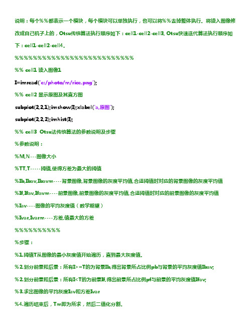
说明：每个%%都表示一个模块，每个模块可以单独执行，也可以将%%去掉整体执行。

将读入图像修改成自己机子上的，Otsu传统算法执行顺序如下：cell1-cell2-cell3,Otsu快速迭代算法执行顺序如下：cell1-cell2-cell4。

%%%%%%%%%%%%%%%%%%%%%%%%%%%% cell1 读入图像1I=imread('e:/photo/m/rice.png');%% cell2显示原图及其直方图subplot(2,2,1);imshow(I);xlabel('a,原图');subplot(2,2,2);imhist(I);%% cell3Otsu法传统算法的参数说明及步骤%参数说明：%M,N---图像大小%TT,T-----阈值,使得方差为最大的阈值%Ib,Ibav,Ibavm----背景图像,背景图像的灰度平均值,合适阈值时对应的背景图像的灰度平均值%If,Ifav,Ifavm----前景图像,前景图像的灰度平均值,合适阈值时对应的前景图像的灰度平均值%Iav----图像的平均灰度值（数学期望）%Ivar,Ivarm----方差,值最大的方差%%%%%%%%%%%步骤：%1.阈值T从图像的最小灰度值开始遍历，直到最大灰度值。

%2.划分前景和后景：所有I>=T的为背景Ib,得出背景所占比例pb与背景的平均灰度值Ibav;%2.划分前景和后景：所有I<T的为前景If,得出前景所占比例pf与前景的平均灰度值Ifav;%3.求出图像的平均灰度Iav和方差Ivar%4.遍历结束后，Tm即为所求，然后二值化分割。

%%%%%%%%%%%%%%%%%%%%%%[M,N]=size(I);Ivarm=0;T=0;Iav=mean(mean(I));tic;for TT=min(min(I)):max(max(I))%划分前景背景Ib=I(I>=TT);pb=length(Ib)/(M*N);Ibav=mean(Ib);If=I(I<TT);pf=length(If)/(M*N);Ifav=mean(If);%求类间方差，并找出最大方差Ivar=pb*pf*(Ibav-Ifav)^2 %lvar=pb*(Ibav-Iav)^2+pf*(Ifav-Iav)^2; if Ivar>IvarmIvarm=Ivar;T=TT;endendtoc;% 输出disp(strcat('大律法计算出的阈值: ',num2str(T)));Iotsu=im2bw(I,double(T)/255);subplot(2,2,2);imshow(Iotsu,[]);xlabel('b,大律法'); %%%%%%%%%%%%%%%%%%%%%%%%%% cel4 OTSU传统算法的快速实现----迭代%参数说明：%M,N---图像大小%T-----阈值(即使得方差为最大的阈值)%gmin,gmax---图像灰度级最小值和最大值%p---图像灰度级概率分布，一维数组长度gmin*gmax%Ibp,Ibav,Ibavm----背景图像灰度级概率,背景图像的灰度平均值,合适阈值时对应的背景图像的灰度平均值%Ifp,Ifav,Ifavm----前景图像灰度级概率,前景图像的灰度平均值,合适阈值时对应的前景图像的灰度平均值%Iav----图像的平均灰度值（数学期望）%Ivar,Ivarm----方差,值最大的方差%%%%%%%%%%%步骤：%1.先求解gmin,gmax,p,Iav,并令Ibp=0,Ibav=0,Ivarm=0;%2.i从gmin+1到gmax+1迭代搜索,(下面为方便说明，使用了序列)Ibp(i)=Ibp(i-1)+p(i),Ibav(i)=(Ibp(i-1)*Ibav(i-1)+i*p(i))/Ibp(i),Ivar(i)=(Ibp(i)*(Iav-Ibav(i))^2)/(1-Ibp(i));%2.判断Iavm是否大于Iav,若是,则i=i+1,重复第2步;若否,则Iavm=Iav,T=i,Ibavm=Ibav,Ifavm=Ifav,i=i+1,重复第2步;%3.迭代结束，T即为所求，二值化分割。

Otsu算法是一种自适应的二值化方法，其主要思想是将图像分成背景和前景两部分，使得背景和前景之间的类间方差最大，而背景和前景内部的类内方差最小。

具体实现步骤如下：
统计图像的灰度直方图，得到每个灰度级别的像素数量。

计算每个灰度级别的归一化概率和平均灰度值。

遍历所有灰度级别，计算每个灰度级别的类内方差和类间方差。

选择使类间方差最大的灰度级别作为阈值进行二值化。

将图像中小于阈值的像素设为0，大于等于阈值的像素设为255。

通过Otsu 算法，可以得到一个自适应的二值化阈值，能够有效地将背景和前景分离，提高图像的对比度和清晰度，常用于图像分割和边缘检测等领域。

OTSU算法学习OTSU公式证明OTSU算法学习 OTSU公式证明1 otsu的公式如下,如果当前阈值为t,w0 前景点所占⽐例w1 = 1- w0 背景点所占⽐例u0 = 前景灰度均值u1 = 背景灰度均值u = w0*u0 + w1*u1 全局灰度均值g = w0(u0-u)*(u0-u) + w1(u1-u)*(u1-u) = w0*(1 – w0)*(u0 - u1)* (u0 - u1)⽬标函数为g, g越⼤,t就是越好的阈值.为什么采⽤这个函数作为判别依据,直观是这个函数反映了前景和背景的差值.差值越⼤,阈值越好.下⾯是⼀段证明g的推导的matlab代码syms w0 u0 u1 %w0 前景均值 u0 前景灰度均值 u1 背景灰度均值%背景均值w1 =1- w0;%全局灰度均值u=w0*u0+w1*u1;%⽬标函数g=w0*(u0-u)*(u0-u)+w1*(u1-u)*(u1-u);%化简的形式g1 =w0*w1*(u0-u1)*(u0-u1);%因式展开a1 = expand(g)%结果是 - u0^2*w0^2 + u0^2*w0 + 2*u0*u1*w0^2 - 2*u0*u1*w0 - u1^2*w0^2 + u1^2*w0a2 = expand(g)%结果是 - u0^2*w0^2 + u0^2*w0 + 2*u0*u1*w0^2 - 2*u0*u1*w0 - u1^2*w0^2 + u1^2*w0%对g进⾏因式分解a2 = factor(g)%结果 -w0*(u0 - u1)^2*(w0 - 1)这⾥是matlab初等代数运算的讲解2 关于最⼤类间⽅差法（otsu）的性能:类间⽅差法对噪⾳和⽬标⼤⼩⼗分敏感，它仅对类间⽅差为单峰的图像产⽣较好的分割效果。

当⽬标与背景的⼤⼩⽐例悬殊时，类间⽅差准则函数可能呈现双峰或多峰，此时效果不好，但是类间⽅差法是⽤时最少的。

3 代码实现public int GetThreshValue(Bitmap image){BitmapData bd = image.LockBits(new Rectangle(0,0, image.Width, image.Height), ImageLockMode.WriteOnly,image.PixelFormat);byte* pt =(byte*)bd.Scan0;int[] pixelNum = new int[256];//图象直⽅图，共256个点byte color;byte* pline;int n, n1, n2;int total;//total为总和，累计值double m1, m2, sum, csum, fmax, sb;//sb为类间⽅差，fmax存储最⼤⽅差值int k, t, q;int threshValue =1;// 阈值int step =1;switch(image.PixelFormat){case PixelFormat.Format24bppRgb:step =3;break;case PixelFormat.Format32bppArgb:step =4;break;case PixelFormat.Format8bppIndexed:step =1;break;}//⽣成直⽅图pline = pt + i * bd.Stride;for(int j =0; j < image.Width; j++){color =*(pline + j * step);//返回各个点的颜⾊，以RGB表⽰pixelNum[color]++;//相应的直⽅图加1}}//直⽅图平滑化for(k =0; k <=255; k++){total =0;for(t =-2; t <=2; t++)//与附近2个灰度做平滑化，t值应取较⼩的值{q = k + t;if(q <0)//越界处理q =0;if(q >255)q =255;total = total + pixelNum[q];//total为总和，累计值}//平滑化，左边2个+中间1个+右边2个灰度，共5个，所以总和除以5，后⾯加0.5是⽤修正值pixelNum[k]=(int)((float)total /5.0+0.5);}//求阈值sum = csum =0.0;n =0;//计算总的图象的点数和质量矩，为后⾯的计算做准备for(k =0; k <=255; k++){//x*f(x)质量矩，也就是每个灰度的值乘以其点数（归⼀化后为概率），sum为其总和sum +=(double)k *(double)pixelNum[k];n += pixelNum[k];//n为图象总的点数，归⼀化后就是累积概率}fmax =-1.0;//类间⽅差sb不可能为负，所以fmax初始值为-1不影响计算的进⾏n1 =0;for(k =0; k <255; k++)//对每个灰度（从0到255）计算⼀次分割后的类间⽅差sb{n1 += pixelNum[k];//n1为在当前阈值遍前景图象的点数if(n1 ==0){continue;}//没有分出前景后景n2 = n - n1;//n2为背景图象的点数//n2为0表⽰全部都是后景图象，与n1=0情况类似，之后的遍历不可能使前景点数增加，所以此时可以退出循环if(n2 ==0){break;}csum +=(double)k * pixelNum[k];//前景的“灰度的值*其点数”的总和m1 = csum / n1;//m1为前景的平均灰度m2 =(sum - csum)/ n2;//m2为背景的平均灰度sb =(double)n1 *(double)n2 *(m1 - m2)*(m1 - m2);//sb为类间⽅差if(sb > fmax)//如果算出的类间⽅差⼤于前⼀次算出的类间⽅差{fmax = sb;//fmax始终为最⼤类间⽅差（otsu）threshValue = k;//取最⼤类间⽅差时对应的灰度的k就是最佳阈值}}image.UnlockBits(bd);image.Dispose();return threshValue;}参考了这篇⽂章4 ⼆维otsu算法下图是⼆维otsu的⽴体图,是对右边的A进⾏⼆维直⽅图统计得到的图像, 遍历区域为5*5.这是对应的matlab代码%统计⼆维直⽅图 i 当前点的亮度 j n*n邻域均值亮度function hist2 = hist2Function(image, n)%初始化255*2565矩阵hist2 = zeros(255,255);[height, width]= size(image);for i =1:heightfor j =1:widthdata = image(i,j);tempSum =0.0;for l =-n:1:nfor m =-n:1:nx = i + l;y = j+m;if x <1x =1;elseif x > widthx = width;endif y <1y =1;elseif y > heighty = height;endtempSum = tempSum + double(image(y,x));endendtempSum = tempSum /((2*n+1)*(2*n+1));hist2(data,floor(tempSum))= hist2(data,floor(tempSum))+1;endend%加载图像imagea = imread('a.bmp');%显⽰图像%imshow(imagea);%显⽰直⽅图%figure;imhist(imagea);%计算⼆维直⽅图hist2 = hist2Function(imagea,2);%显⽰⼆维直⽅图[x,y]=meshgrid(1:1:255);mesh(x,y,hist2)<灰度图象的⼆维Otsu⾃动阈值分割法.pdf> 这篇⽂章讲解的不错.⽂章这⾥有下载下⾯⽤数学语⾔表达⼀下i :表⽰亮度的维度j : 表⽰点区域均值的维度w0: 表⽰在阈值(s,t)时所占的⽐例w1: 表⽰在阈值(s,t)时, 所占的⽐例u0(u0i, u0j): 表⽰在阈值(s,t)时时的均值.u0时2维的u1(u1i, u1j): 表⽰在阈值(s,t)时的均值.u1时2维的uT: 全局均值和⼀维otsut函数类似的⽬标函数sb = w0(u0-uT)*(u0-uT)’ + w1(u1-uT)*(u1-uT)’= w0[(u0i-uTi)* (u0i-uTi) + (u0j-uTj)* (u0j-uTj)] + w1[(u1i-uTi)* (u1i-uTi) + (u1j-uTj)* (u1j-uTj)]这⾥是代码实现.出⾃这篇⽂章:int histogram[256][256];double p_histogram[256][256];double Pst_0[256][256];//Pst_0⽤来存储概率分布情况double Xst_0[256][256];//存储x⽅向上的均值⽮量int OTSU2d(IplImage * src){int height = src->height;int width = src->width;long pixel = height * width;int i,j;for(i =0;i <256;i++)//初始化直⽅图for(j =0; j <256;j++)histogram[i][j]=0;}IplImage * temp = cvCreateImage(cvGetSize(src),8,1);cvSmooth(src,temp,CV_BLUR,3,0);for(i =0;i < height;i++)//计算直⽅图{for(j =0; j < width;j++){int data1 = cvGetReal2D(src,i,j);int data2 = cvGetReal2D(temp,i,j);histogram[data1][data2]++;}}for(i =0; i <256;i++)//直⽅图归⼀化for(j =0; j <256;j++)p_histogram[i][j]=(histogram[i][j]*1.0)/(pixel*1.0);Pst_0[0][0]= p_histogram[0][0];for(i =0;i <256;i++)//计算概率分布情况for(j =0;j <256;j++){double temp =0.0;if(i-1>=0)temp = temp + Pst_0[i-1][j];if(j-1>=0)temp = temp + Pst_0[i][j-1];if(i-1>=0&& j-1>=0)temp = temp - Pst_0[i-1][j-1];temp = temp + p_histogram[i][j];Pst_0[i][j]= temp;}Xst_0[0][0]=0* Pst_0[0][0];for(i =0; i <256;i++)//计算x⽅向上的均值⽮量for(j =0; j <256;j++){double temp =0.0;if(i-1>=0)temp = temp + Xst_0[i-1][j];if(j-1>=0)temp = temp + Xst_0[i][j-1];if(i-1>=0&& j-1>=0)temp = temp - Xst_0[i-1][j-1];temp = temp + i * p_histogram[i][j];Xst_0[i][j]= temp;}double Yst_0[256][256];//存储y⽅向上的均值⽮量Yst_0[0][0]=0* Pst_0[0][0];for(i =0; i <256;i++)//计算y⽅向上的均值⽮量for(j =0; j <256;j++){double temp =0.0;if(i-1>=0)temp = temp + Yst_0[i-1][j];if(j-1>=0)temp = temp + Yst_0[i][j-1];if(i-1>=0&& j-1>=0)temp = temp - Yst_0[i-1][j-1];temp = temp + j * p_histogram[i][j];Yst_0[i][j]= temp;}int threshold1;int threshold2;double variance =0.0;double maxvariance =0.0;for(i =0;i <256;i++)//计算类间离散测度for(j =0;j <256;j++){longdouble p0 = Pst_0[i][j];longdouble v0 = pow(((Xst_0[i][j]/p0)-Xst_0[255][255]),2)+ pow(((Yst_0[i][j]/p0)-Yst_0[255][255]),2);longdouble p1 = Pst_0[255][255]-Pst_0[255][j]-Pst_0[i][255]+Pst_0[i][j];longdouble vi = Xst_0[255][255]-Xst_0[255][j]-Xst_0[i][255]+Xst_0[i][j];longdouble vj = Yst_0[255][255]-Yst_0[255][j]-Yst_0[i][255]+Yst_0[i][j];longdouble v1 = pow(((vi/p1)-Xst_0[255][255]),2)+pow(((vj/p1)-Yst_0[255][255]),2);variance = p0*v0+p1*v1;if(variance > maxvariance){maxvariance = variance;threshold1 = i;threshold2 = j;}}//printf("%d %d",threshold1,threshold2);return(threshold1+threshold2)/2;}总结: ⼆维otsu算法得到⼀个阈值,然后对图像做⼆值化.仍然不能解决光照不均匀⼆值化的问题.⽐⼀维otsu效果好⼀些,但不是很明显.这个算法的亮点在于考虑的点的附近区域的均值.。

t-matrice scatter matlab code -回复tmatrice scatter matlab code是一种用于绘制散点图的Matlab代码。

散点图是一种用于可视化两个变量之间关系的图表，它通常用于识别数据之间的趋势、相关性或者异常值。

tmatrice scatter matlab code提供了一种简便的方式来创建和定制散点图。

在本文中，我们将一步一步地回答有关tmatrice scatter matlab code的问题，介绍其基本用法以及其他可能的用途和扩展技巧。

第一步：安装和配置Matlab要使用tmatrice scatter matlab code，您需要首先安装并配置Matlab 在本地机器上。

您可以从MathWorks官方网站下载Matlab并按照提供的指示进行安装。

安装完成后，您需要验证安装是否成功，并设置Matlab 的工作环境。

第二步：了解tmatrice scatter matlab code的语法和参数在使用tmatrice scatter matlab code之前，我们首先需要了解它的语法和可用的参数。

tmatrice scatter matlab code的基本语法如下：scatter(x, y, s, c)其中，- x和y是两个向量，分别表示散点图中点的x坐标和y坐标。

- s是一个数值或者向量，表示散点的大小。

如果s是一个数值，所有散点的大小将相同；如果s是一个向量，每个散点的大小将根据向量中的值进行定制。

- c是一个数值或者向量，表示散点的颜色。

如果c是一个数值，所有散点的颜色将相同；如果c是一个向量，每个散点的颜色将根据向量中的值进行定制。

第三步：创建散点图有了tmatrice scatter matlab code的语法和参数，我们现在可以创建一个简单的散点图来演示它的用法。

假设我们有以下的数据：x = [1, 2, 3, 4, 5]y = [1, 4, 9, 16, 25]下面是使用tmatrice scatter matlab code创建散点图的代码：scatter(x, y)运行上述代码后，您将看到一个由x和y坐标构成的散点图。

matlab常⽤算法⼤全Matlab ⾼级算法程序代码汇总⼀、灰⾊预测模型matlab程序% renkou1=renkou(:,1);%年末常住⼈⼝数% renkou2=renkou(:,2);%户籍⼈⼝% renkou3=renkou(:,3);%⾮户籍⼈⼝% shjian=1979:2010;%以上数据⾃⼰给x0=renkou2';n=length(x0);lamda=x0(1:n-1)./x0(2:n)range=minmax(lamda)x1=cumsum(x0)for i=2:nz(i)=0.5*(x1(i)+x1(i-1));endB=[-z(2:n)',ones(n-1,1)];Y=x0(2:n)';u=B\Yx=dsolve('Dx+a*x=b','x(0)=x0');x=subs(x,{'a','b','x0'},{u(1),u(2),x1(1)});yuce1=subs(x,'t',[0:n-1]);digits(6),y=vpa(x) %为提⾼预测精度，先计算预测值，再显⽰微分⽅程的解yuce=[x0(1),diff(yuce1)] epsilon=x0-yuce %计算残差delta=abs(epsilon./x0) %计算相对误差rho=1-(1-0.5*u(1))/(1+0.5*u(1))*lamda %计算级⽐偏差值%以深圳⼈⼝数据得到预测模型及预测误差相关数据lamda =Columns 1 through 80.9741 0.9611 0.9419 0.8749 0.9311 0.90930.9302 0.9254Columns 9 through 160.9245 0.9278 0.9442 0.9376 0.9127 0.91480.9332 0.9477Columns 17 through 240.9592 0.9445 0.9551 0.9562 0.9594 0.94610.9469 0.9239Columns 25 through 310.9140 0.9077 0.9243 0.9268 0.9312 0.94460.9618range =0.8749 0.9741x1 =1.0e+003 *Columns 1 through 80.0313 0.0634 0.0967 0.1322 0.1727 0.2162 0.2641 0.3155Columns 9 through 160.3711 0.4313 0.4961 0.5647 0.6380 0.7182 0.8059 0.8999Columns 17 through 240.9990 1.1024 1.2119 1.3265 1.4463 1.57121.7033 1.8427Columns 25 through 321.99362.1588 2.3407 2.5375 2.7499 2.97803.2194 3.4705u =-0.066531.3737y =-472.117+503.377*exp(.664533e-1*t)yuce =Columns 1 through 831.2600 34.5876 36.9641 39.5040 42.2183 45.1192 48.2194 51.5326 Columns 9 through 1655.0734 58.8576 62.9017 67.2238 71.8428 76.7792 82.0548 87.6928 Columns 17 through 2493.7183 100.1578 107.0397 114.3945 122.2547 130.6550 139.6324 149.2267 Columns 25 through 32159.4802 170.4382 182.1492 194.6649 208.0405 222.3352 237.6121 253.9386 epsilon =Columns 1 through 80 -2.4976 -3.5741 -4.0540 -1.6983 -1.5992-0.3594 -0.0826Columns 9 through 160.5266 1.2824 1.9183 1.4262 1.3772 3.44085.63526.2772Columns 17 through 245.4417 3.2222 2.4203 0.2055 -2.4047 -5.7350 -7.5924 -9.7767Columns 25 through 32-8.5502 -5.3082 -0.2192 2.1651 4.3395 5.7348 3.8379 -2.9086delta =Columns 1 through 80 0.0778 0.1070 0.1144 0.0419 0.03670.0075 0.0016Columns 9 through 160.0095 0.0213 0.0296 0.0208 0.0188 0.0429 0.0643 0.0668Columns 17 through 240.0549 0.0312 0.0221 0.0018 0.0201 0.0459 0.0575 0.0701Columns 25 through 320.0567 0.0321 0.0012 0.0110 0.0204 0.0251 0.0159 0.0116rho =Columns 1 through 8-0.0411 -0.0271 -0.0066 0.0650 0.0049 0.0282 0.0058 0.0110Columns 9 through 160.0119 0.0084 -0.0091 -0.0020 0.0245 0.0223 0.0027 -0.0128Columns 17 through 24-0.0251 -0.0094 -0.0208 -0.0219 -0.0254 -0.0111-0.0119 0.0126Columns 25 through 310.0232 0.0300 0.0122 0.0095 0.0048 -0.0095-0.0280⼆、遗传算法程序代码% Optimizing a function using Simple Genetic Algorithm with elitist preserved%Max f(x1,x2)=100*(x1*x1-x2).^2+(1-x1).^2; -2.0480<=x1,x2<=2.0480 % Author: Wang Yonglin (wylin77@/doc/eb41cd3fe109581b6bd97f19227916888486b98d.html ) clc;clear all;format long;%设定数据显⽰格式%初始化参数T=100;%仿真代数N=80;% 群体规模pm=0.05;pc=0.8;%交叉变异概率umax=2.048;umin=-2.048;%参数取值范围L=10;%单个参数字串长度，总编码长度2Lbval=round(rand(N,2*L));%初始种群bestv=-inf;%最优适应度初值%迭代开始for ii=1:T%解码，计算适应度for i=1:Ny1=0;y2=0;for j=1:1:Ly1=y1+bval(i,L-j+1)*2^(j-1);endx1=(umax-umin)*y1/(2^L-1)+umin;for j=1:1:Ly2=y2+bval(i,2*L-j+1)*2^(j-1);endx2=(umax-umin)*y2/(2^L-1)+umin;obj(i)=100*(x1*x1-x2).^2+(1-x1).^2; %⽬标函数xx(i,:)=[x1,x2];endfunc=obj;%⽬标函数转换为适应度函数p=func./sum(func);q=cumsum(p);%累加[fmax,indmax]=max(func);%求当代最佳个体if fmax>=bestvbestv=fmax;%到⽬前为⽌最优适应度值bvalxx=bval(indmax,:);%到⽬前为⽌最佳位串optxx=xx(indmax,:);%到⽬前为⽌最优参数endBfit1(ii)=bestv; % 存储每代的最优适应度%%%%遗传操作开始%轮盘赌选择for i=1:(N-1)r=rand;tmp=find(r<=q);newbval(i,:)=bval(tmp(1),:);endnewbval(N,:)=bvalxx;%最优保留bval=newbval;%单点交叉for i=1:2:(N-1)cc=rand;if ccpoint=ceil(rand*(2*L-1));%取得⼀个1到2L-1的整数ch=bval(i,:); bval(i,point+1:2*L)=bval(i+1,point+1:2*L);bval(i+1,point+1:2*L)=ch(1,point+1:2*L);endendbval(N,:)=bvalxx;%最优保留%位点变异mm=rand(N,2*L)mm(N,:)=zeros(1,2*L);%最后⼀⾏不变异，强制赋0bval(mm)=1-bval(mm);end%输出plot(Bfit1);% 绘制最优适应度进化曲线bestv %输出最优适应度值optxx %输出最优参数三、种⼦群算法程序代码%declare the parameters of the optimizationmax_iterations = 1000;no_of_particles = 50;dimensions = 1;delta_min = -0.003;delta_max = 0.003;c1 = 1.3;c2 = 1.3;%initialise the particles and teir velocity componentsfor count_x = 1:no_of_particlesfor count_y = 1:dimensionsparticle_position(count_x,count_y) = rand*10;particle_velocity(count_x,count_y) = rand;p_best(count_x,count_y) = particle_position(count_x,count_y); end end%initialize the p_best_fitness arrayfor count = 1:no_of_particlesp_best_fitness(count) = -1000;end%particle_position%particle_velocity%main particle swrm routinefor count = 1:max_iterations%find the fitness of each particle%change fitness function as per equation requiresd and dimensions for count_x = 1:no_of_particles%x = particle_position(count_x,1);%y = particle_position(count_x,2);%z = particle_position(count_x,3);%soln = x^2 - 3*y*x + z;%x = particle_position(count_x);%soln = x^2-2*x+1;x = particle_position(count_x);soln = x-7;if soln~=0current_fitness(count_x) = 1/abs(soln); elsecurrent_fitness =1000;endend%decide on p_best etc for each particlefor count_x = 1:no_of_particlesif current_fitness(count_x) >p_best_fitness(count_x)p_best_fitness(count_x) = current_fitness(count_x);for count_y = 1:dimensionsp_best(count_x,count_y) = particle_position(count_x,count_y); endendend%decide on the global best among all the particles[g_best_val,g_best_index] = max(current_fitness);%g_best contains the position of teh global bestfor count_y = 1:dimensionsg_best(count_y) = particle_position(g_best_index,count_y); end%update the position and velocity compponentsfor count_x = 1:no_of_particlesfor count_y = 1:dimensionsp_current(count_y) = particle_position(count_x,count_y);endfor count_y = 1:dimensionsparticle_velocity(count_y) = particle_velocity(count_y) + c1*rand*(p_best(count_y)-p_current(count_y)) + c2*rand*(g_best(count_y)-p_current(count_y));particle_positon(count_x,count_y) = p_current(count_y)+particle_velocity(count_y);endendendg_bestcurrent_fitness(g_best_index)clear all, clc % pso exampleiter = 1000; % number of algorithm iterationsnp = 2; % number of model parametersns = 10; % number of sets of model parametersWmax = 0.9; % maximum inertial weightWmin = 0.4; % minimum inertial weightc1 = 2.0; % parameter in PSO methodologyc2 = 2.0; % parameter in PSO methodologyPmax = [10 10]; % maximum model parameter valuePmin = [-10 -10]; % minimum model parameter valueVmax = [1 1]; % maximum change in model parameterVmin = [-1 -1]; % minimum change in model parametermodelparameters(1:np,1:ns) = 0; % set all model parameter estimates for all model parameter sets to zero modelparameterchanges(1:np,1:ns) = 0; % set all change in model parameter estimates for all model parameter sets to zero bestmodelparameters(1:np,1:ns) = 0; % set best model parameter estimates for all model parameter sets to zero setbestcostfunction(1:ns) = 1e6; % set best cost function of each model parameter set to a large number globalbestparameters(1:np) = 0; % set best model parameter values for all model parameter sets to zero bestparameters = globalbestparameters'; % best model parameter values for all model parameter sets (to plot) globalbestcostfunction = 1e6; % set best cost function for all model parameter sets to a large numberi = 0; % indicates ith algorithm iterationj = 0; % indicates jth set of model parametersk = 0; % indicates kth model parameterfor k = 1:np % initializationfor j = 1:nsmodelparameters(k,j) = (Pmax(k)-Pmin(k))*rand(1) + Pmin(k); % randomly distribute model parameters modelparameterchanges(k,j) = (Vmax(k)-Vmin(k))*rand(1) + Vmin(k); % randomly distribute change in model parameters endendfor i = 2:iterfor j = 1:nsx = modelparameters(:,j);% calculate cost functioncostfunction = 105*(x(2)-x(1)^2)^2 + (1-x(1))^2;if costfunctionbestmodelparameters(:,j) = modelparameters(:,j);setbestcostfunction(j) = costfunction;四、模拟退⽕算法% for d=1:50 %循环10次发现最⼩路径为4.115，循环50次有3次出现4.115 T_max=80; %input('please input the start temprature');T_min=0.001; %input('please input the end temprature');iter_max=100;%input('please input the most interp steps on the fit temp');s_max=100; %input('please input the most steady steps ont the fit temp');T=T_max;load .\address.txt;order1=randperm(size(address,1))';%⽣成初始解。