ANSYS高级工程有限元分析范例精选——之一
- 格式:pdf
- 大小:2.68 MB
- 文档页数:83

ansys有限元分析工程实例大作业————————————————————————————————作者:————————————————————————————————日期:辽宁工程技术大学有限元软件工程实例分析题目基于ANSYS钢桁架桥的静力分析专业班级建工研16-1班(结构工程)学号 471620445姓名日期 2017年4月15日基于ANSYS钢桁架桥的静力分析摘要:本文采用ANSYS分析程序,对下承式钢桁架桥进行了有限元建模;对桁架桥进行了静力分析,作出了桁架桥在静载下的结构变形图、位移云图、以及各个节点处的结构内力图(轴力图、弯矩图、剪切力图),找出了结构的危险截面。
关键词:ANSYS;钢桁架桥;静力分析;结构分析。
引言:随着现代交通运输的快速发展,桥梁兴建的规模在不断的扩大,尤其是现代铁路行业的快速发展更加促进了铁路桥梁的建设,一些新建的高速铁路桥梁可以达到四线甚至是六线,由于桥面和桥身的材料不同导致其受力情况变得复杂,这就需要桥梁需要有足够的承载力,足够的竖向侧向和扭转刚度,同时还应具有良好的稳定性以及较高的减震降噪性,因此对其应用计算机和求解软件快速进行力学分析了解其受力特性具有重要的意义。
1、工程简介某一下承式简支钢桁架桥由型钢组成,顶梁及侧梁,桥身弦杆,底梁分别采用3种不同型号的型钢,结构参数见表1,材料属性见表2。
桥长32米,桥高5.5米,桥身由8段桁架组成,每个节段4米。
该桥梁可以通行卡车,若只考虑卡车位于桥梁中间位置,假设卡车的质量为4000kg,若取一半的模型,可以将卡车对桥梁的作用力简化为P1,P2,和P3,其中P1=P3=5000N,P2=10000N,见图2,钢桥的形式见图1,其结构简图见图3。
图1钢桥的形式图2桥梁的简化平面模型(取桥梁的一半)图3刚桁架桥简图所用的桁架杆件有三种规格,见表1表1 钢桁架杆件规格杆件截面号形状规格顶梁及侧梁 1 工字形400X400X12X12桥身弦杆 2 工字形400X300X12X12底梁 3 工字形400X400X16X16所用的材料属性,见表2表2 材料属性参数钢材弹性模量EX泊松比PRXY 0.3密度DENS 78002 模型构建将下承式钢桁梁桥的各部分杆件,包括顶梁及侧梁,桥身弦杆,底梁均采用BEAM188单元,此空间梁单元可以考虑所模拟杆件的轴向变形; 定义了一套材料属性,各类杆件为钢材,其对应的参数如表2所示;根据表1中的杆件规格定义了三种梁单元截面,根据表1分别定义在相应的梁上;建模时直接建立节点和单元,在后续按照先建节点再建杆的次序一次建模。

有 限 元 分 析 作 业作业名称 换热管的热分析姓 名学 号 3060612061班 级 06机电(3)班宁波理工学院题目:换热管的热分析:本题要确定的是一个换热器中带管板结构答对换热管的温度分布和应力分布。
单程换热器的其中一根换热管和与其相连的两端管板结构,壳程介质为热蒸汽,管程介质为液体操作介质,热换管材料为不锈钢,膨胀系数为616.5610-⨯℃1-,泊松比为0.3,弹性模量为51.7210MPa ⨯,热导率为15.1/(W m ⋅℃);管板材料也为不锈钢,膨胀系数为617.7910-⨯℃1-,泊松比为0.3,弹性模量为51.7310MPa ⨯,热导率为15.1/(W m ⋅℃),壳程蒸汽温度为250℃,表面传热系数为23000/W m ℃,壳程压力为8.1MPa,管程液体温度200℃,表面传热系数为426/(W m ⋅℃);管程压力为5.7MPa.换热管内径为0.01295m,外径0.01905m,管板厚度0.05m,换热管长度为0.5m,部分管板材料长和宽均为0.013m.换热管和管板结构如下图:1. 定义工作文件名和文件标题(1) 定义工作文件名:执行Utility Menu-File-Chang Jobname(2) 定义工作标题:执行Utility Menu-File-Change Tile(3) 关闭坐标符合现实:执行Utility Menu-PlotCtrls-WindowsCtrols-Window Options-Location of triad ,单击OK 按钮。
2. 定义材料属性和单元类型(1) 定义单元类型,执行Main Menu-Preprocessor-Element Type-Add 弹出Element Type 对话框,分别选择Theml solid和Brick 20node 90选项,单击OK按钮.如下图1-1所示:1-1(2)定义材料属性执行:Main menu-Preprocessor-Material Props-Material models,在Define material model behavior对话框中,双击Structual-Linear-Elastic-Isotropic,在弹出的对话框中,EX后输入1.73E11,在PRXY后输入0.3,单击OK按钮,如下图1-2所示:1-2连续单击Thermal expansion-Secant coefficient-Isotropic,在弹出的对话框中,ALPX 后输入17.79E-6,单击OK按钮。

Ansys有限元课程设计问题一:飞机机翼振动模态分析机翼模型沿着长度方向具有不规则形状,而且其横截面是由直线和曲线构成(如图所示)。
机翼一端固定于机身上,另一端则自由悬挂。
机翼材料的常数为:弹性模量E=0.26GPa,泊松比m=0.3,密度r=886kg/m^3一、操作步骤:1.选取5个keypoint,A(0,0,0)为坐标原点,同时为翼型截面的尖点;2.B(2,0,0)为下表面轮廓截面直线上一点,同时是样条曲线BCDE的起点;3.D(1.9,0.45,0)为样曲线上一点;4.C(2.3,0.2,0)为样条曲线曲率最大点,样条曲线的顶点;5.E(1,0.25,0)与点A构成直线,斜率为0.25;6.通过点A、B做直线和点B、C、D、E作样条曲线就构成了截面的形状。
沿Z 方向拉伸,就得到机翼的实体模型;7.创建截面如图:机翼材料的常数为:弹性模量E=0.26GPa,泊松比m=0.3,密度r=886kg/m^3 8.定义网格密度并进行网格划分:选择面单元PLANE42和体单元SOLID45进行划分网格求解。
面网格选择单元尺寸为0.00625,体网格划分时按单元数目控制网格划分,选择单元数目为109.对模型施加约束,由于机翼一端固定在机身上所以在机翼截面的一端所有节点施加位移和旋转约束二、有限元处理结果及分析:机翼的各阶模态及相应的变形:一阶振动模态图:二阶振动模态图:三阶振动模态图:四阶振动模态图:五阶振动模态图:命令流:/FILNAM,MODAL/TITLE,Modal analysis of a modal airplane wing /PMETH,OFF,0KEYW,PR_STRUC,1/UIS,MSGPOP,3/PREP7ET,1,PLANE42ET,2,SOLID45MP,EX,1,380012MP,PRXY,1,0.3MP,DENS,1,1.033E-3K,1,K,2,2K,3,2.3,0.2K,4,1.9,0.45K,5,1,0.25/TRIAD,OFF/PNUM,KP,1LSTR,1,2LSTR,5,1BSPLIN,2,3,4,5,,,-1,0,,-1,-0.25,, AL,1,2,3ESIZE,0.25MSHKEY,0MSHAPE,0,2DAMESH,1SAVEESIZE,,10TYPE,2VEXT,1,,,0,0,10/SOLUANTYPE,MODAL MODOPT,SUBSP,5,,,,OFF EQSLV,SPARMXPAND,5,,,,0.001 LUMPM,0PSTRES,0ESEL,U,TYPE,,1NSEL,S,LOC,Z,0D,ALL,ALLALLSEL,ALLSOLVE/POST1SET,LISTSET,FIRSTPLDI,,ANMODE,10,0.5,,0FINISH13/EXIT,ALL问题二:内六角扳手静力分析内六角扳手在日常生产生活当中运用广泛,先受1000N的力产生的扭矩作用,然后在加上200N力的弯曲,分析算出在这两种外载作用下扳手的应力分布。

工程软件应用及设计实习报告实习时间:一.实习目的:1.熟悉工程软件在实际应用中具体的操作流程与方法,同时结合所学知识对理论内容进行实际性的操作.2.培养我们动手实践能力,将理论知识同实际相结合的能力,提高大家的综合能力,便于以后就业及实际应用.3.工程软件的应用是对课本所学知识的拓展与延伸,对我们专业课的学习有很大的提高,也是对我们进一步的拔高与锻炼. 二.实习内容(一)用ANSYS软件进行输气管道的有限元建模与分析计算分析模型如图1所示承受内压:1.0e8 PaR1=0.3R2=0.5管道材料参数:弹性模量E=200Gpa;泊松比v=0.26.图1受均匀内压的输气管道计算分析模型(截面图)题目解释:由于管道沿长度方向的尺寸远远大于管道的直径,在计算过程中忽略管道的断面效应,认为在其方向上无应变产生.然后根据结构的对称性,只要分析其中1/4即可.此外,需注意分析过程中的单位统一.操作步骤1.定义工作文件名和工作标题1.定义工作文件名.执行Utility Menu-File→Chang Jobname-3070611062,单击OK按钮.2.定义工作标题.执行Utility Menu-File→Change Tile-chentengfei3070611062,单击OK 按钮.3.更改目录.执行Utility Menu-File→change the working directory –D/chen2.定义单元类型和材料属性1.设置计算类型ANSYS Main Menu: Preferences →select Structural →OK2.选择单元类型.执行ANSYS Main Menu→Preprocessor →Element Type→Add/Edit/Delete →Add →select Solid Quad 8node 82 →applyAdd/Edit/Delete →Add →select Solid Brick 8node 185 →OKOptions…→select K3: Plane strain →OK→Close如图2所示,选择OK接受单元类型并关闭对话框.图23.设置材料属性.执行Main Menu→Preprocessor →Material Props →Material Models →Structural →Linear →Elastic →Isotropic,在EX框中输入2e11,在PRXY框中输入0.26,如图3所示,选择OK并关闭对话框.图33.创建几何模型1. 选择ANSYS Main Menu: Preprocessor →Modeling →Create →Keypoints →In Active CS →依次输入四个点的坐标:input:1(0.3,0),2(0.5,0),3(0,0.5),4(0,0.3) →OK2. 生成管道截面.ANSYS 命令菜单栏: Work Plane>Change Active CS to>Global Spherical →ANSYS Main Menu: Preprocessor →Modeling →Create →Lines →In Active Coord →依次连接1,2,3,4点→OK 如图4图4Preprocessor →Modeling →Create →Areas →Arbitrary →By Lines →依次拾取四条边→OK →ANSYS 命令菜单栏: Work Plane>Change Active CS to>Global Cartesian 如图5图53.拉伸成3维实体模型Preprocessor →Modeling→operate→areas→along normal输入2,如图6所示图64.生成有限元网格Preprocessor →Meshing →Mesh Tool→V olumes Mesh→Tet→Free,.采用自由网格划分单元.执行Main Menu-Preprocessor-Meshing-Mesh-V olume-Free,弹出一个拾取框,拾取实体,单击OK按钮.生成的网格如图7所示.图75.施加载荷并求解1.施加约束条件.执行Main Menu-Solution-Apply-Structural-Displacement-On Areas,弹出一个拾取框,拾取前平面,单击OK按钮,弹出如图8所示的对话框,选择“U Y”选项,单击OK按钮.图8同理,执行Main Menu-Solution-Apply-Structural-Displacement-On Areas,弹出一个拾取框,拾取左平面,单击OK按钮,弹出如图8所示的对话框,选择“U X”选项,单击OK按钮.2.施加载荷.执行Main Menu-Solution-Apply-Structural-Pressure-On Areas,弹出一个拾取框,拾取内表面,单击OK按钮,弹出如图10所示对话框,如图所示输入数据1e8,单击OK按钮.如图9所示.生成结构如图10图9图103.求解.执行Main Menu-Solution-Solve-Current LS,弹出一个提示框.浏览后执行file-close,单击OK按钮开始求解运算.出现一个【Solution is done】对话框是单击close按钮完成求解运算.6.显示结果1.显示变形形状.执行Main Menu-General Posproc-Plot Results-Deformed Shape,弹出如图11所示的对话框.选择“Def+underformed”单选按钮,单击OK按钮.生成结果如图12所示.图11图122.列出节点的结果.执行Main Menu-General Posproc-List Results-Nodal Solution,弹出如图13所示的对话框.设置好后点击OK按钮.生成如图14所示的结果图13图143.浏览节点上的V on Mises应力值.执行Main Menu-General Posproc-Plot Results-Contour Plot-Nodal Solu,弹出如图15所示对话框.设置好后单击OK按钮,生成结果如图16所示.图15图167.以扩展方式显示计算结果1.设置扩展模式.执行Utility Menu-Plotctrls-Style-Symmetry Expansion,弹出如图17所示对话框.选中“1/4 Dihedral Sym”单选按钮,单击OK按钮,生成结果如图18所示.图17图182.以等值线方式显示.执行Utility Menu-Plotctrls-Device Options,弹出如图19所示对话框,生成结果如图20所示.图19图20结果分析通过图18可以看出,在分析过程中的最大变形量为418E-03m,最大的应力为994E+08Pa,最小应力为257E+09Pa.应力在内表面比较大,所以在生产中应加强内表面材料的强度.。

.ANSYS有限元事例剖析报告ANSYS剖析报告一、ANSYS简介 :ANSYS软件是融构造、流体、电场、磁场、声场剖析于一体的大型通用有限元剖析软件。
由世界上最大的有限元剖析软件企业之一的美国 ANSYS开发,它能与多半 CAD软件接口,实现数据的共享和互换,如Pro/Engineer, NASTRAN,AutoCAD等,是现代产品设计中的高级CAE工具之一。
本实验我们用的是ANSYS14.0软件。
二、剖析模型:y详细以下:a以下图, L/B=10,a= 0.2B ,bBb= (0.5-2)a,比较 b 的变化对b x 最大应力 x的影响。
aL三、模型剖析:该问题是平板受力后的应力剖析问题。
我们经过使用ANSYS软件求解,第一要成立上图所示的平面模型,而后在平板一段施加位移约束,另一端施加载荷,最后求解模型,用图形显示,即可获取实验结果。
四、ANSYS求解:求解过程以 b=0.5a=0.02 为例:1.成立工作平面, X-Y 平面内画长方形,L=1,B=0.1,a=0.02,b=0.5a=0.01; (操作流程: preprocessor →modeling →create →areas →rectangle )2.依据椭圆方程,利用描点法画椭圆曲线,为了方便的获取更多的椭圆上的点,我们利用 C++程序进行编程。
程序语句以下:运转结果以下:本问题(b=0.5a=0.01 )中,x 在[0,0.02] 上每隔 0.002 取一个点, y 值对应于第一行结果。
由点坐标能够画出这 11 个点,用 reflect命令对于 y 轴对称,而后一次圆滑连结这 21 个点,再用直线连结两个端点,便获取关闭的半椭圆曲线。
(操作流程: create →keypoints→o n active CS →挨次输入椭圆上各点坐标地点→ reflect →create→s plines through keypoints→creat→lines→获取关闭曲线)。
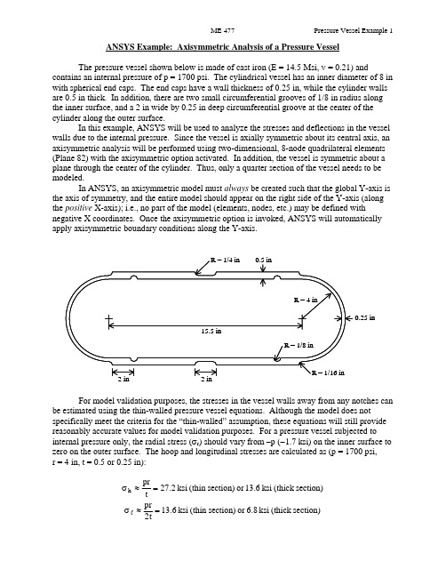
ANSYS Example: Axisymmetric Analysis of a Pressure VesselThe pressure vessel shown below is made of cast iron (E = 14.5 Msi, ν = 0.21) andcontains an internal pressure of p = 1700 psi. The cylindrical vessel has an inner diameter of 8 in with spherical end caps. The end caps have a wall thickness of 0.25 in, while the cylinder walls are 0.5 in thick. In addition, there are two small circumferential grooves of 1/8 in radius along the inner surface, and a 2 in wide by 0.25 in deep circumferential groove at the center of the cylinder along the outer surface.In this example, ANSYS will be used to analyze the stresses and deflections in the vessel walls due to the internal pressure. Since the vessel is axially symmetric about its central axis, an axisymmetric analysis will be performed using two-dimensional, 8-node quadrilateral elements (Plane 82) with the axisymmetric option activated. In addition, the vessel is symmetric about a plane through the center of the cylinder. Thus, only a quarter section of the vessel needs to be modeled.In ANSYS, an axisymmetric model must always be created such that the global Y-axis is the axis of symmetry, and the entire model should appear on the right side of the Y-axis (along the positive X-axis); i.e., no part of the model (elements, nodes, etc.) may be defined withnegative X coordinates. Once the axisymmetric option is invoked, ANSYS will automatically apply axisymmetric boundary conditions along the Y-axis.R = 1/16 inR = 1/8 inR = 1/4 in 0.5 in0.25 inR = 4 in2 in 2 in 15.5 inFor model validation purposes, the stresses in the vessel walls away from any notches can be estimated using the thin-walled pressure vessel equations. Although the model does notspecifically meet the criteria for the “thin-walled” assumption, these equations will still provide reasonably accurate values for model validation purposes. For a pressure vessel subjected to internal pressure only, the radial stress (σr ) should vary from –p (−1.7 ksi) on the inner surface to zero on the outer surface. The hoop and longitudinal stresses are calculated as (p = 1700 psi, r = 4 in, t = 0.5 or 0.25 in):section)(thick ksi 13.6or section)(thin ksi 27.2tpr h =≈σ section)(thick ksi 6.8or section)(thin ksi 6.31t2pr =≈σlANSYS Analysis:Start ANSYS Product Launcher, set the Working Directory to C:\temp, define Job Name as‘Pressure Vessel’, and click Run. Then define Title and Preferences.Utility MenuÆFileÆChange Jobname…Æ Enter ‘Pressure_Vessel’ Æ OKUtility MenuÆFileÆChange Title…Æ Enter ‘Stress Analysis of an Axisymmetric Pressure Vessel’ Æ OKANSYS Main MenuÆPreferencesÆ Preferences for GUI Filtering Æ Select ‘Structural’ and ‘h-method’ Æ OKEnter the Preprocessor to define the model geometry:Define Element Type (Axisymmetric Option) and Material Properties.ANSYS Main MenuÆPreprocessor ÆElement Type Æ Add/Edit/Delete Æ Add… ÆStructural Solid Quad 8 node 82 (PLANE82) (define ‘Element type reference number’ as 1) ÆOK Æ Click Options… Æ Select ‘Axisymmetric’ for K3 (Element behavior) Æ OK Æ Close ANSYS Main MenuÆPreprocessorÆMaterial PropsÆ Material Models Æ Double Click Structural Æ Linear Æ Elastic Æ Isotropic Æ Enter 14.5e6 for EX and 0.21 for PRXY Æ Click OK Æ Click Exit (under ‘Material’)Begin creating the geometry by defining two Circles for the spherical endcap, and Subtract Areas to create the vessel wall.ANSYS Main MenuÆPreprocessorÆModelingÆCreateÆAreasÆCircleÆ Solid Circle Æ Enter 0 for WP X, 0 for WP Y, and 4 for Radius Æ Apply Æ Enter 0 for WP X, 0 for WP Y, and 4.25 for Radius Æ OKANSYS Main MenuÆPreprocessorÆModelingÆOperateÆBooleansÆSubtractÆAreas Æ Select (with the mouse) Area 2 (bigger circle) Æ OK Æ Select Area 1 (smaller circle) Æ OKCreate Lines through the center of the Circles and Divide the Areas along these Lines.ANSYS Main MenuÆPreprocessorÆModelingÆCreateÆLinesÆLinesÆ Straight line Æ Click on the Keypoints on the outer circle which are on the X-axis to create a Line parallel to the X-axis (Circles are divided into four arcs by Ansys, with a Keypoint placed at the end of each arc). Similarly, click on the Keypoints on the outer circle which are on the Y-axis to create a Line parallel to the Y-axis Æ OKANSYS Main MenuÆPreprocessorÆModelingÆOperateÆBooleansÆDivideÆArea by Line Æ Select (with the mouse) the remaining Area (annulus)Æ OK Æ Select the two Lines that we have created Æ OKANSYS Main MenuÆPreprocessorÆModelingÆDeleteÆ Area and Below Æ Select the three Areas in the first, second, and third quadrants Æ OKDefine two Rectangles to create the walls of the cylindrical portion of the vessel (thick and thin sections). Define a Circle to create the circumferential groove on the inside of the vessel. ANSYS Main MenuÆPreprocessorÆModelingÆCreateÆAreasÆRectangleÆ By Dimensions Æ Enter 4 and 4.5 for X-coordinates and 0 and 7.75 for Y-coordinates Æ Click Apply Æ Enter 4.25 and 4.5 for X-coordinates and 6.75 and 7.75 for Y-coordinates Æ OK ANSYS Main MenuÆPreprocessorÆModeling ÆCreateÆAreasÆCircleÆ Solid Circle Æ Enter 4 for WP X, 2 for WP Y, and 1/8 for Radius Æ OKSubtract Areas to eliminate unused segments, and then Add all Areas to create a single Area for meshing.ANSYS Main MenuÆPreprocessorÆModelingÆOperateÆBooleansÆSubtractÆAreas Æ Select (with the mouse) the bigger rectangle Æ OK Æ Select the small rectangle and circle Æ OKANSYS Main MenuÆPreprocessorÆModelingÆOperateÆBooleansÆAddÆ Areas Æ Select ‘Pick All’ Æ OKCreate Line Fillets at the two transitions between the thick and thin sections.Utility Menu Æ Plot ÆLinesUtility Menu Æ Plot CtrlsÆNumbering…Æ Click ‘Line numbers’ On Æ OKANSYS Main MenuÆPreprocessorÆModelingÆCreateÆLinesÆ Line Fillet Æ Select (with the mouse) the two Lines near the lower Fillet Æ OK Æ Enter 1/16 for Fillet radius ÆApply Æ Select the two Lines near the upper Fillet Æ OK Æ Enter 1/4 for Fillet radius Æ OK Create Areas within the two Fillets and add these Areas to the main Area. First zoom in on the area of interest using the plot controls.ANSYS Main MenuÆPreprocessorÆModelingÆCreateÆAreasÆArbitraryÆ By Lines Æ Select (with the mouse) the Fillet and adjacent two Lines Æ OKRepeat for the other Fillet.ANSYS Main MenuÆPreprocessorÆModelingÆOperateÆBooleansÆAddÆ Areas Æ Select ‘Pick All’ Æ OKUtility Menu Æ Plot ÆLinesThe geometry should appear as shown below in the figure on the left.In this example, the irregular geometry will be Free Meshed with Quad Elements. Better control of Element sizing and distribution can be obtained with Mapped Meshing, but this would require that additional sub-Areas be defined within the main Area that have a regular (four-sided) geometry. Using Free Meshing, all Elements in the model will be approximately the same size. In the first run, we will choose a Global Size (approximate Element edge length) of 0.1 in. ANSYS Main MenuÆPreprocessorÆMeshingÆ MeshTool Æ Under ‘Size Controls: Global’ click Set Æ Enter 0.1 for ‘Element edge length’ ÆOK Æ Under ‘Mesh:’ select Areas, Quad and Free Æ Click Mesh Æ Select (with the mouse) the Area Æ OKEnter the Solution Menu to define boundary conditions and loads and run the analysis: ANSYS Main MenuÆSolutionÆAnalysis TypeÆ New Analysis Æ Select Static Æ OK The Boundary Conditions and Loads can now be applied. ANSYS will automatically apply the Axisymmetric Boundary Conditions along the Y-axis. However, we must apply the Symmetry Boundary Conditions along the upper edge of the model. Finally, the Pressure can be applied on all lines that make up the inner surface of the vessel. The magnitude should be input as the actual value – no reduction is needed to account for axisymmetry (ANSYS automatically makes the necessary adjustment of Loads in an Axisymmetric model).ANSYS Main MenuÆSolutionÆDefine LoadsÆApplyÆStructuralÆDisplacement ÆSymmetry B.C.Æ On Lines Æ Select the Line on top of the model (19) Æ OKANSYS Main MenuÆSolutionÆDefine LoadsÆApplyÆStructuralÆPressureÆ On Lines Æ Select (with the mouse) all the Lines on the inside of the vessel (20,12,16,17 and 2) ÆOK Æ Enter 1700 for ‘Load PRES value’ Æ OKThe pressure will be indicated by arrows, as shown above in the figure on the right.Save the Database and initiate the Solution using the current Load Step (LS).ANSYS Toolbar Æ SAVE_DBANSYS Main MenuÆSolutionÆSolveÆ Current LS Æ OK Æ Close the information window when solution is done Æ Close the /STATUS Command windowEnter the General Postprocessor to examine the results:First, plot the Deformed Shape.ANSYS Main MenuÆGeneral PostprocÆPlot ResultsÆ Deformed Shape Æ Select Def + undeformed Æ OKA Contour Plot of any stress component can be created. The radial, hoop (tangential), and longitudinal stresses should be checked to verify the model. Also, stress values at any particular node can be checked by using the “Query Results” command, selecting the desired component, and then picking the appropriate node. For this model, along the cylindrical portion of the vessel, x represents the radial direction, y represents the longitudinal direction, and z represents the hoop (tangential) direction. Powergraphics must be disabled to query results at nodes. ANSYS Toolbar Æ POWRGRPH Æ Select OFF Æ OKANSYS Main MenuÆGeneral PostprocÆPlot ResultsÆContour PlotÆ Nodal Solu ÆSelect ‘Stress’ and ‘X-Component of stress’ (or Y or Z) Æ OKANSYS Main MenuÆGeneral PostprocÆQuery ResultsÆ Nodal Solution Æ Select‘Stress’ and ‘X-direction SX’ (or SY or SZ) Æ OK Æ Select Nodes in the region of interest (may be helpful to zoom in on region)Compare the finite element stresses to the values calculated using the thin-wall equations. If the values are within reason (away from notches, etc.), proceed. For the purposes of failure analysis, we must select an appropriate failure theory. A plot of the von Mises stress is useful for identifying critical locations in the vessel. However, since the vessel is made of cast iron (brittle material), the “Maximum-Normal-Stress” failure criterion may be more appropriate (or Coulomb-Mohr or other similar failure theories). Create Contour Plots of the von Mises and 1st Principal stresses.ANSYS Main MenuÆGeneral PostprocÆPlot ResultsÆContour PlotÆ Nodal Solu ÆSelect ‘Stress’ and ‘von Mises stress’ Æ OKANSYS Main MenuÆGeneral PostprocÆPlot ResultsÆContour PlotÆ Nodal Solu ÆSelect ‘Stress’ and ‘1st Principal stress’ Æ OKThe plot of the model can be expanded around the axisymmetric axis to get a better view of the full model. For this plot, Powergraphics must be enabled.ANSYS Toolbar Æ POWRGRPH Æ Select ON Æ OKUtility Menu Æ PlotCtrlsÆStyleÆ Symmetry Expansion Æ 2-D Axi-Symmetric… Æ Select ‘Full expansion’ Æ OKNote the locations of the maximum stresses in the vessel. Are the critical locations where you would expect them to be? If not, why? Do you think the current model is accurate, or might there be some discretization error? Record the magnitudes and locations of the maximum stresses, and then refine the mesh and re-run the analysis to check for possible discretization error.。
有限元分析一个厚度为20mm的带孔矩形板受平面内张力,如下图所示。
左边固定,右边受载荷p=20N/mm作用,求其变形情况200100P20一个典型的ANSYS分析过程可分为以下6个步骤:①定义参数②创建几何模型③划分网格④加载数据⑤求解⑥结果分析1定义参数1.1指定工程名和分析标题(1)启动ANSYS软件,选择File→Change Jobname命令,弹出如图所示的[Change Jobname]对话框。
(2)在[Enter new jobname]文本框中输入“plane”,同时把[New log and error files]中的复选框选为Yes,单击确定(3)选择File→Change Title菜单命令,弹出如图所示的[Change Title]对话框。
(4)在[Enter new title]文本框中输入“2D Plane Stress Bracket”,单击确定。
1.2定义单位在ANSYS软件操作主界面的输入窗口中输入“/UNIT,SI”1.3定义单元类型(1)选择Main Menu→Preprocessor→Element Type→Add/Edit/Delete命令,弹出如图所示[Element Types]对话框。
(2)单击[Element Types]对话框中的[Add]按钮,在弹出的如下所示[Library of Element Types]对话框。
(3)选择左边文本框中的[Solid]选项,右边文本框中的[8node 82]选项,单击确定,。
(4)返回[Element Types]对话框,如下所示(5)单击[Options]按钮,弹出如下所示[PLANE82 element type options]对话框。
(6)在[Element behavior]下拉列表中选择[Plane strs w/thk]选项,单击确定。
(7)再次回到[Element Types]对话框,单击[close]按钮结束,单元定义完毕。
Ansys有限元课程设计问题一:飞机机翼振动模态分析机翼模型沿着长度方向具有不规则形状,而且其横截面是由直线和曲线构成(如图所示)。
机翼一端固定于机身上,另一端则自由悬挂。
机翼材料的常数为:弹性模量E=0.26GPa,泊松比m=0.3,密度r=886kg/m^3一、操作步骤:1.选取5个keypoint,A(0,0,0)为坐标原点,同时为翼型截面的尖点;2.B(2,0,0)为下表面轮廓截面直线上一点,同时是样条曲线BCDE的起点;3.D(1.9,0.45,0)为样曲线上一点;4.C(2.3,0.2,0)为样条曲线曲率最大点,样条曲线的顶点;5.E(1,0.25,0)与点A构成直线,斜率为0.25;6.通过点A、B做直线和点B、C、D、E作样条曲线就构成了截面的形状。
沿Z 方向拉伸,就得到机翼的实体模型;7.创建截面如图:机翼材料的常数为:弹性模量E=0.26GPa,泊松比m=0.3,密度r=886kg/m^3 8.定义网格密度并进行网格划分:选择面单元PLANE42和体单元SOLID45进行划分网格求解。
面网格选择单元尺寸为0.00625,体网格划分时按单元数目控制网格划分,选择单元数目为109.对模型施加约束,由于机翼一端固定在机身上所以在机翼截面的一端所有节点施加位移和旋转约束二、有限元处理结果及分析:机翼的各阶模态及相应的变形:一阶振动模态图:二阶振动模态图:三阶振动模态图:四阶振动模态图:五阶振动模态图:命令流:/FILNAM,MODAL/TITLE,Modal analysis of a modal airplane wing /PMETH,OFF,0KEYW,PR_STRUC,1/UIS,MSGPOP,3/PREP7ET,1,PLANE42ET,2,SOLID45MP,EX,1,380012MP,PRXY,1,0.3MP,DENS,1,1.033E-3K,1,K,2,2K,3,2.3,0.2K,4,1.9,0.45K,5,1,0.25/TRIAD,OFF/PNUM,KP,1LSTR,1,2LSTR,5,1BSPLIN,2,3,4,5,,,-1,0,,-1,-0.25,, AL,1,2,3ESIZE,0.25MSHKEY,0MSHAPE,0,2DAMESH,1SAVEESIZE,,10TYPE,2VEXT,1,,,0,0,10/SOLUANTYPE,MODAL MODOPT,SUBSP,5,,,,OFF EQSLV,SPARMXPAND,5,,,,0.001 LUMPM,0PSTRES,0ESEL,U,TYPE,,1NSEL,S,LOC,Z,0D,ALL,ALLALLSEL,ALLSOLVE/POST1SET,LISTSET,FIRSTPLDI,,ANMODE,10,0.5,,0FINISH13/EXIT,ALL问题二:内六角扳手静力分析内六角扳手在日常生产生活当中运用广泛,先受1000N的力产生的扭矩作用,然后在加上200N力的弯曲,分析算出在这两种外载作用下扳手的应力分布。
角托架的有限元建模与分析一 、模型介绍本模型是关于一个角托架的简单加载,线性静态结构分析问题,托架的具体形状和尺寸如图所示。
托架左上方的销孔被焊接完全固定,其右下角的销孔受到锥形压力载荷,角托架材料为Q235A 优质钢。
角托架材料参数为:弹性模量366E e psi =;泊松比0.27ν=托架图(厚度:0.5)二、问题分析因为角托架在Z 方向尺寸相对于其在X,Y 方向的尺寸来说很小,并且压力荷载仅作用在X,Y 平面上,因此可以认为这个分析为平面应力状态。
三、模型建立3.1 指定工作文件名和分析标题(1)选择菜单栏Utility Menu →File →Jobname 命令.系统将弹出Jobname(修改文件名)对话框,输入bracket(2)定义分析标题GUI :Utility Menu>Preprocess>Element Type>Add/Edit/Delete 执行命令后,弹出对话框,输入stress in a bracket 作为ANSYS 图形显示时的标题。
3.2设置计算类型Main Menu: Preferences … →select Structural → OK3.3定义单元类型PLANE82 GUI :Main Menu →Preprocessor →Element Type →Add/Edit/Delete 命令,系统将弹出Element Types 对话框。
单击Add 按钮,在对话框左边的下拉列表中单击Structural Solid →Quad 8node 82,选择8节点平面单元PLANE82。
单击ok ,Element Types 对话框,单击Option ,在Element behavior 后面窗口中选取Plane strs w/thk 后单击ok 完成定义单元类型。
3.4定义单元实常数GUI:Main Menu: Preprocessor →Real Constants→Add/Edit/Delete,弹出定义实常数对话框,单击Add,弹出要定义实常数单元对话框,选中PLANE82单元后,单击OK→定义单元厚度对话框,在THK中输入0.5.3.5定义材料特性GUI:Main Menu: Preprocessor →Material Props →Material Models →Structural →Linear →Elastic →Isotropic →输入EX=30e6, 泊松比v=0.27 → OK3.6建立几何模型(1)定义矩形GUI:Main Menu: Preprocessor →Modeling →Create →Area –Rectangle→by Dimensions →依次输入X1=0,X2=6,Y1=-1,Y2=1→Apply生成第一个矩形→输入X1=0,X2=6,Y1=-1,Y2=3单击OK生成第二个矩形。