GMG-VD1.0软件使用说明书

现代电气控制系统安装与调试虚拟仿真软件软件说明书北京欧倍尔软件技术开发有限公司2020 年10 月地址：北京海淀区清河永泰园甲1号建金商厦515-516室邮编：100085地址：北京海淀区清河永泰园甲1号建金商厦515-516室 邮编：100085目录一、软件介绍 ............................................................................................................................. 3 二、功能介绍 .. (3)1.软件场景 .......................................................................................................................... 3 2.知识点预习...................................................................................................................... 4 3.思考题功能...................................................................................................................... 5 4.设备展示 .......................................................................................................................... 5 5.帮助功能 .......................................................................................................................... 6 6.录像功能 .......................................................................................................................... 7 7.返回主页 .......................................................................................................................... 8 8.评分功能 .......................................................................................................................... 8 9.博图通讯 .......................................................................................................................... 9 三、操作步骤 (10)1.安装模式 ........................................................................................................................ 10 2.连线模式 ........................................................................................................................ 10 3.运行模式 ........................................................................................................................ 12 四、实训内容 (13)（一）三相交流异步电动机的点动控制电路实验 ...................................................... 13 （二）三相交流异步电动机的单向连续转动的控制电路实验 .................................. 17 （三）接触器联锁的三相交流异步电动机正、反转控制电路实验 .......................... 21 （四）按钮联锁的三相交流异步电动机正、反转控制电路的实验 .......................... 25 （五）按钮、接触器联锁的三相交流异步电动机正、反转控制电路实验.............. 29 （六）两地控制电路实验 .............................................................................................. 34 （七）电动机往返行程控制电路实验 .......................................................................... 38 （八）普通车床控制电路的实验 .................................................................................. 43 （九）点动与连续转动电路实验 .................................................................................. 47 （十）多台（3台电动机）电动机的顺序控制电路实验 ........................................... 51 （十一）三相交流异步电动机Y-△（手动切换）启动控制电路实验 ..................... 56 （十二）PLC 控制交通灯的实训 .................................................................................. 60 （十三）控制电机顺序启动实验 .................................................................................. 63 （十四）控制三相异步电动机Y-△启动电路实验 .. (65)地址：北京海淀区清河永泰园甲1号建金商厦515-516室 邮编：100085 一、软件介绍北京欧倍尔软件研发的现代电气控制系统安装与调试虚拟仿真软件，可仿真现代电气控制和自动生产线实训操作的各类控制环节，学生可在博图、三菱等配套软件中进行PLC 编程，在仿真软件内搭建好相关场景后，通过与PLC 编程软件的通讯，在仿真软件内对各类实验进行相关调试，可重复操作直至得出满意结果，该实训系统用于技能大赛的训练可提升参赛选手的操作熟练度和技能水平，改变了传统的受限于设备数量和场地大小的教学模式，极大地提升了学生的学习热情和学习效果。

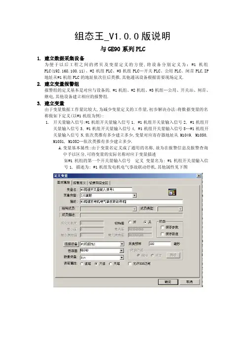
组态王_V1.0.0版说明与GE90系列PLC1.建立数据采集设备为便于以后工程之间的拷贝及变量定义的方便,将设备分别定义为：#1机组PLC(192.168.100.11)、#2机组PLC、#3机组PLC…开关PLC、公用PLC、闸首PLC,IP 地址从#1机组PLC的地址依次往后类推,其他通讯设备根据需要现场定义.2.建立变量报警组报警组的定义基本是对应与设备的,#1机组、#2机组、#3机组…公用、开关站、闸首、继电,其他设备建立相应的报警组.3.建立变量由于变量数据工作量比较大,为减少变量定义的工作量,初步解决办法:将数据变量的名称做如下定义(以#1机组为例):1.开关量输入信号:#1机组开关量输入信号1, #1机组开关量输入信号2, #1机组开关量输入信号3, #1机组开关量输入信号4, #1机组开关量输入信号5…#1机组开关量输入信号N,依次类推有多少建立多少,变量对应寄存器地址从M1049, M1050, M1051, M1052…依次类推有多少建立多少.A.变量基本属性:由于变量名定义成了通用的名称,故为在报警信息及报警查询中予以区分,可将变量的实际名称对应于变量描述如#1机组的第一个开关量输入信号定义变量名为: #1机组开关量输入信号1, 描述为: #1机组发电机电气事故联动停机,其他属性见下图B.变量报警定义(见下图)选择对应的报警组选择报警类型:现报警类型均选择为改变方式.C.变量记录和安全区(见下图)记录项选择不记录.安全区不做选择.2.开关量输出信号:输出信号定义同输入信号定义方法,变量地址直接取硬件地址.3.模拟量输入信号(地址从R5901开始)A:基本属性(见下图)变量名: 使用实际名称变量类型:I/O实数描述:对应变量名工程值转换:最小/大值,最小/大原始值均先定义为0—32000,变换灵敏度为0,最小/大值到现场根据实际情况修改,原始值同最小值.采集频率设为1000ms.数据类型为根据数据实际类型,选择有/无符号类型.读写属性为只读.B.报警定义模拟量一般不定义其报警属性如现场有需要可根据实际情况设置其报警的低低限,低限,高限,高高限,报警组相应选择.C.变量记录和安全区(见下图)记录项选择定时记录,没10分钟记录一次.注:由于曲线显示需要,机组的P,Q定义为每次采集记录.安全区不做选择.4.上位机控制信号:对时命令:#1机组PLC对时秒(R501), #1机组PLC对时分(R502), #1机组PLC对时时(R503), #1机组PLC对时日(R504), #1机组PLC对时月(R505), #1机组PLC对时年(R506).变量读写类型选择读写控制命令:#1机组PLC下行标志(R214)#1机组控制对象(R215):设定不同的值区分控制的对象.#1机组控制性质(R216): 设定不同的值做出不同的控制.#1机组命令来源(R217):预留.#1机组设定有功_无功(R218): 设定不同的值分别投入有/无功调节.#1机组PID下发实际值(R219):需要机组实际调节到的实际符合值.以上控制命令变量均要在其记录和安全区选项中选择生成事件.变量读写类型选择读写5.968E上送遥信,遥测信号:遥测:R5001—R5256:最小/大原始值均为968E对应设备模版中的最小/大值,变换灵敏度为0,最小/大值到现场根据实际情况修改,原始值同最小值.遥信:R5527--R5512:968E送到PLC的为一个字,需要PLC将每个字解析出来.6.虚拟信号:A.报警码寄存器地址从M2441开始往后类推…虚拟DI寄存器地址紧接实际开入信号地址,其他属性同开关量输入信号. 虚拟AI寄存器地址紧接实际模拟量输入信号地址,绿色预留.*1机组状态说明：0--不定态，1--发电态, 2--空转态, 3--停机态，4--空载态, 5--调相态, 6--检修态7.模拟量输入信号品质:寄存器地址从QQ1001开始往后类推,变量名及描述均为对应实际模拟量名称后加上品质两字.报警定义:选择改变,开到关输入好,关到开输入坏.其他同开关量输入信号.8.继电保护装置通讯信号:根据模版直接导入即可,注意模版中的设备名称要跟实际建立的设备名称一直,否则无法导入.注:对应于每一个通讯设备,均需要定义一通讯状态变量,如: #1机组PLC通讯状态,寄存器类型选择 CommErr,为1时表示通讯中断在报警定义中如下图2所示1.2.4.系统配置1.运行参数配置运行系统基准频率:300毫秒.时间量更新频率:500毫秒.禁止推出运行环境. (系统正式运行时)禁止任务切换. (系统正式运行时)禁止ALT键. (系统正式运行时)2.报警参数配置A.文件配置B.数据库配置AA.文件配置—报警格式注意变量名及变量描述长度AB.文件配置—操作格式注意变量名及变量描述长度AC.文件配置—登陆格式3.历史记录配置5.画面说明1.主接线画面:用于监视主接线开关及刀闸位置,各点的电气量测量显示,以及每台机组的风闸,锁锭,开机条件,冷却水信号2.机组单元接线及电气遥测A.单元接线B.电气遥测画面3.机组温度及水机遥测量显示画面4.机组遥信信号显示画面。

Package‘CNVRG’October12,2022Title Dirichlet Multinomial Modeling of Relative Abundance DataVersion1.0.0Maintainer Joshua Harrison<*******************************>DescriptionImplements Dirichlet multinomial modeling of relative abundance data using functionality pro-vided by the'Stan'software.The purpose of this package is to provide a user friendly way to in-terface with'Stan'that is suitable for those new to modeling.For more regarding the model-ing mathematics and computational techniques we use see our publication in Molecular Ecol-ogy Resources titled'Dirichlet multinomial modeling outperforms alternatives for analy-sis of ecological count data'(Harrison et al.2020<doi:10.1111/1755-0998.13128>).License GPL-3Encoding UTF-8LazyData trueRoxygenNote7.1.1Biarch trueDepends R(>=3.4.0)Imports methods,Rcpp(>=0.12.0),rstan(>=2.18.1),vegan,rstantools(>=2.1.1),tibbleLinkingTo BH(>=1.66.0),Rcpp(>=0.12.0),RcppEigen(>=0.3.3.3.0),RcppParallel(>=5.0.1),rstan(>=2.18.1),StanHeaders(>=2.18.0)SystemRequirements GNU makeRepository CRANNeedsCompilation yesAuthor Joshua Harrison[aut,cre](<https:///0000-0003-2524-0273>), Vivaswat Shastry[aut](<https:///0000-0002-7294-5607>),W.John Calder[aut](<https:///0000-0002-8923-1803>),C.Alex Buerkle[aut](<https:///0000-0003-4222-8858>)Date/Publication2021-09-0404:40:06UTC1R topics documented:CNVRG-package (2)cnvrg_HMC (2)cnvrg_VI (4)diff_abund (5)diversity_calc (6)extract_pi_quantiles (8)extract_point_estimate (9)fungi (10)indexer (11)isd_transform (11)Index14 CNVRG-package The’CNVRG’package.DescriptionThis package implements Dirichlet multinomial modeling of relative abundance data using func-tionality provided by the’Stan’software.The purpose of this package is to provide a user friendly way to interface with’Stan’that is suitable for those new modelling.ReferencesStan Development Team(2018).RStan:the R interface to Stan.R package version2.18.2. cnvrg_HMC Perform Hamiltonian Monte Carlo samplingDescriptionThis function uses a compiled Dirichlet multinomial model and performs Hamiltonian Monte Carlo sampling of posteriors using’Stan’.After sampling it is important to check e the summary function and shinystan to do this.If you use this function then credit’Stan’and’RStan’along with this package.Usagecnvrg_HMC(countData,starts,ends,algorithm="NUTS",chains=2,burn=500,samples=1000,thinning_rate=2,cores=1,params_to_save=c("pi","p"))ArgumentscountData A matrix or data frame of counts.Thefirstfield should be sample names and the subsequentfields should be integer data.Data should be arranged so that thefirst n rows correspond to one treatment group and the next n rows correspondwith the next treatment group,and so on.The row indices for thefirst and lastsample in these groups are fed into this function via’starts’and’ends’.starts A vector defining the indices that correspond to thefirst sample in each treatment group.The indexer function can help with this.ends A vector defining the indices that correspond to the last sample in each treatment group.The indexer function can help with this.algorithm The algorithm to use when sampling.Either’NUTS’or’HMC’or’Fixed_param’.If unsure,then be like a squirrel.This is"No U turn sampling".The abbreviationis from’Stan’.chains The number of chains to run.burn The warm up or’burn in’time.samples How many samples from the posterior to save.thinning_rate Thinning rate to use during sampling.cores The number of cores to use.params_to_save The parameters from which to save samples.Can be’p’,’pi’,’theta’.DetailsIt can be helpful to use the indexer function to automatically identify the indices needed for the ’starts’and’ends’parameters.See the vignette for an example.Warning:data must be input in the correct organized format or this function will not provide accu-rate results.See vignette if you are unsure how to organize data.Warning:depending upon size of data to be analyzed this function can take a very long time to run.ValueAfitted’Stan’object that includes the samples from the parameters designated.Examples#simulate an OTU tablecom_demo<-matrix(0,nrow=10,ncol=10)com_demo[1:5,]<-c(rep(3,5),rep(7,5))#Alternates3and7com_demo[6:10,]<-c(rep(7,5),rep(3,5))#Reverses alternationfornames<-NA4cnvrg_VIfor(i in1:length(com_demo[1,])){fornames[i]<-paste("otu_",i,sep="")}sample_vec<-NAfor(i in1:length(com_demo[,1])){sample_vec[i]<-paste("sample",i,sep="_")}com_demo<-data.frame(sample_vec,com_demo)names(com_demo)<-c("sample",fornames)#These are toy data,many more samples,multiple chains,and a longer burn#are likely advisable for real data.fitstan_HMC<-cnvrg_HMC(com_demo,starts=c(1,6),ends=c(5,10),chains=1,burn=100,samples=150,thinning_rate=2)cnvrg_VI Perform variational inference samplingDescriptionThis function uses a compiled Dirichlet multinomial model and performs variational inference esti-mation of posteriors using’Stan’.Evaluating the performance of variational inference is currently under development per our understanding.Please roll over to the’Stan’website and see if new diagnostics are available.If you use this function then credit’Stan’and’RStan’along with this package.Usagecnvrg_VI(countData,starts,ends,algorithm="meanfield",output_samples=500,params_to_save=c("pi","p"))ArgumentscountData A matrix or data frame of counts.Thefirstfield should be sample names and the subsequentfields should be integer data.Data should be arranged so that thefirst n rows correspond to one treatment group and the next n rows correspondwith the next treatment group,and so on.The row indices for thefirst and lastsample in these groups are fed into this function via’starts’and’ends’.diff_abund5 starts A vector defining the indices that correspond to thefirst sample in each treatment group.The indexer function can help with this.ends A vector defining the indices that correspond to the last sample in each treatment group.The indexer function can help with this.algorithm The algorithm to use when performing variational inference.Either’meanfield’or’fullrank’.The former is the default.output_samples The number of samples from the approximated posterior to save.params_to_save The parameters from which to save samples.Can be’p’,’pi’,’theta’.DetailsIt can be helpful to use the indexer function to automatically identify the indices needed for the ’starts’and’ends’parameters.See the vignette for an example.Warning:data must be input in the correct organized format or this function will not provide accu-rate results.See vignette if you are unsure how to organize data.Warning:depending upon size of data to be analyzed this function can take a very long time to run.ValueAfitted’Stan’object that includes the samples from the parameters designated.Examples#simulate an OTU tablediff_abund Calculate features with different abundances between treatmentgroupsDescriptionThis function determines which features within the matrix that was modeled differ in relative abun-dance among treatment groups.Pass in a model object,with samples for pi parameters.This function only works for pi parameters.Usagediff_abund(model_out,countData,prob_threshold=0.05)Argumentsmodel_out Output of CNVRG modeling functions,including cnvrg_HMC and cnvrg_VI countData Dataframe of count data that was modeled.Should be exactly the same as those data modeled!Thefirstfield should be sample name and integer count datashould be in all otherfields.This is passed in so that the names offields can beused to make the output of differential relative abundance testing more readable.prob_threshold Probability threshold,below which it is considered that features had a high prob-ability of differing between groups.Default is0.05.DetailsThe output of this function gives the proportion of samples that were greater than zero after sub-tracting the two relevant posterior distributions.Therefore,values that are very large or very small denote a high certainty that the distributions subtracted differ.If this concept is not clear,then read Harrison et al.2020’Dirichlet multinomial modeling outperforms alternatives for analysis of microbiome and other ecological count data’in Molecular Ecology Resources.For a simple explanation,see this video:https://use.vg/OSVhFJThe posterior probability distribution of differences is also output.These samples can be useful for plotting or other downstream analyses.Finally,a list of data frames describing the features that differed among treatment comparisons is output,with the probability of differences and the magnitude of those differences(the effect size)included.ValueA dataframe with thefirstfield denoting the treatment comparison(e.g.,treatment1vs.2)andsubsequentfields stating the proportion of samples from the posterior that were greater than zero (called"certainty of diffs").Note that each treatment group is compared to all other groups,which leads to some redundancy in output.A list,called ppd_diffs,holding samples from the posterior probability distribution of the differences is also output.Finally,a list of dataframes describing results for only those features with a high probability of differing is output(this list is named: features_that_differed).Examples#simulate an OTU tablecom_demo<-matrix(0,nrow=10,ncol=10)com_demo[1:5,]<-c(rep(3,5),rep(7,5))#Alternates3and7com_demo[6:10,]<-c(rep(7,5),rep(3,5))#Reverses alternationfornames<-NAfor(i in1:length(com_demo[1,])){fornames[i]<-paste("otu_",i,sep="")}sample_vec<-NAfor(i in1:length(com_demo[,1])){sample_vec[i]<-paste("sample",i,sep="_")}com_demo<-data.frame(sample_vec,com_demo)names(com_demo)<-c("sample",fornames)out<-cnvrg_VI(com_demo,starts=c(1,6),ends=c(5,10))diff_abund_test<-diff_abund(model_out=out,countData=com_demo)diversity_calc Calculate diversity entropies for each replicateDescriptionCalculate Shannon’s or Simpson’s indices for each replicate while propagating uncertainty in rela-tive abundance estimates through calculations.Usagediversity_calc(model_out,countData,params="pi",entropy_measure="shannon",equivalents=T)Argumentsmodel_out Output of CNVRG modeling functions,including cnvrg_HMC and cnvrg_VI or isd_transformcountData Dataframe of count data that was modeled.Should be exactly the same as those data modeled!Thefirstfield should be sample name and integer count datashould be in all otherfields.This is passed in so that the names offields can beused to make the output of differential relative abundance testing more readable.params Parameter for which to calculate diversity,can be’p’or’pi’or both(e.g., c("pi","p"))entropy_measureDiversity entropy to use,can be one of’shannon’or’simpson’equivalents Convert entropies into number equivalents.Defaults to true.See Jost(2006), "Entropy and diversity"DetailsTakes as input either afitted Stan object from the cnvrg_HMC or cnvrg_VI functions,or the output of isd_transform.As always,doublecheck the results to ensure the function has output reasonable values.Note that because there are no zero values and all proportion estimates are non zero there is a lot of information within the modeled data.Because diversity entropies are measures of information content,this means there will be a much higher entropy estimate for modeled data than the raw count data.However,patterns of variation in diversity should be similar among treatment groups for modeled and raw data.ValueA list that has samples from posterior distributions of entropy metricsExamples#simulate an OTU tablecom_demo<-matrix(0,nrow=10,ncol=10)com_demo[1:5,]<-c(rep(3,5),rep(7,5))#Alternates3and7com_demo[6:10,]<-c(rep(7,5),rep(3,5))#Reverses alternationfornames<-NAfor(i in1:length(com_demo[1,])){fornames[i]<-paste("otu_",i,sep="")}8extract_pi_quantiles sample_vec<-NAfor(i in1:length(com_demo[,1])){sample_vec[i]<-paste("sample",i,sep="_")}com_demo<-data.frame(sample_vec,com_demo)names(com_demo)<-c("sample",fornames)out<-cnvrg_VI(com_demo,starts=c(1,6),ends=c(5,10))diversity_calc(model_out=out,params=c("pi","p"),countData=com_demo,entropy_measure= shannon )extract_pi_quantiles Extract quantiles of pi parametersDescriptionProvides quantiles of pi parameters for each feature and treatment group.Usageextract_pi_quantiles(model_out,probs=c(0.05,0.5,0.95))Argumentsmodel_out Output of CNVRG modeling functions,including cnvrg_HMC and cnvrg_VI probs A vector of quantilesValueA list specifying quantiles for each feature in each treatment group.Examples#simulate an OTU tablecom_demo<-matrix(0,nrow=10,ncol=10)com_demo[1:5,]<-c(rep(3,5),rep(7,5))#Alternates3and7com_demo[6:10,]<-c(rep(7,5),rep(3,5))#Reverses alternationfornames<-NAfor(i in1:length(com_demo[1,])){fornames[i]<-paste("otu_",i,sep="")}sample_vec<-NAfor(i in1:length(com_demo[,1])){sample_vec[i]<-paste("sample",i,sep="_")}com_demo<-data.frame(sample_vec,com_demo)names(com_demo)<-c("sample",fornames)out<-cnvrg_VI(com_demo,starts=c(1,6),ends=c(5,10))extract_pi_quantiles(model_out=out,probs=c(0.05,0.5,0.95))extract_point_estimate9 extract_point_estimateExtract point estimates of multinomial and Dirichlet parametersDescriptionProvides the mean value of posterior probability distributions for parameters.Usageextract_point_estimate(model_out,countData,params=c("pi","p"))Argumentsmodel_out Output of CNVRG modeling functions,including cnvrg_HMC and cnvrg_VI countData The count data modeled.params Parameters to be extracted,either pi(Dirichlet)or p(multinomial).ValueA list of of point estimates for model parameters.If both multinomial and Dirichlet parameters arerequested then they will be named elements of a list.Examples#simulate an OTU tablecom_demo<-matrix(0,nrow=10,ncol=10)com_demo[1:5,]<-c(rep(3,5),rep(7,5))#Alternates3and7com_demo[6:10,]<-c(rep(7,5),rep(3,5))#Reverses alternationfornames<-NAfor(i in1:length(com_demo[1,])){fornames[i]<-paste("otu_",i,sep="")}sample_vec<-NAfor(i in1:length(com_demo[,1])){sample_vec[i]<-paste("sample",i,sep="_")}com_demo<-data.frame(sample_vec,com_demo)names(com_demo)<-c("sample",fornames)out<-cnvrg_VI(com_demo,starts=c(1,6),ends=c(5,10))extract_point_estimate(model_out=out,countData=com_demo)10fungi fungi Fungal endophytes of Astragalus lentiginosus grown near Reno,NVDescriptionFungal endophytes of Astragalus lentiginosus grown near Reno,NVUsagefungiFormatA data frame with columns:treatment A categorical variable describing if a plant was treated with a slurry of endophyte in-oculum and whether it was positive or negative for Alternaria fulva.Otu10Contains count data.Otu100Contains count data.Otu11Contains count data.Otu12Contains count data.Otu4Contains count data.Otu40Contains count data.Otu42Contains count data.Otu54Contains count data.Otu58Contains count data.Otu6Contains count data.Otu62Contains count data.Otu7Contains count data.Otu70Contains count data.Otu71Contains count data.Otu72Contains count data.Otu74Contains count data.Otu76Contains count data.Otu77Contains count data.Otu79Contains count data.Otu86Contains count data.Otu9Contains count data.Otu92Contains count data.Otu94Contains count data.Otu96Contains count data.Otu97Contains count data.Otu99Contains count data.indexer11SourceJoshua G.Harrison,https:///content/10.1101/608729v1.fullExamples##Not run:fungi##End(Not run)indexer Determine indices for treatment groupsDescriptionThis function determines the indices for thefirst and last replicates within a vector describing treat-ment group.Usageindexer(x)Argumentsx Vector input.ValueA list with two named elements that contain start and end indices.Examplesindexer(c(rep("treatment1",5),rep("treatment2",5)))isd_transform Transform data into estimates of absolute abundances using an ISDDescriptionIf an internal standard(ISD)has been added to samples such that the counts for that standard are representative of the same absolute abundance,then the ISD can be used to transform relative abundance data such that they are proportional to absolute abundances(Harrison et al.2020).This function performs this division while preserving uncertainty in relative abundance estimates of both the ISD and the other features present.Usageisd_transform(model_out,isd_index,countData,format="stan")Argumentsmodel_out Output of CNVRG modeling functions,including cnvrg_HMC and cnvrg_VI isd_index The index for thefield with information for the internal standard.countData The count data modeled.format The output format.Can be either’or’samples’or’ml’."samples"outputs sam-ples from the posterior probability distribution,the last option("ml")outputs themean of posterior samples for each parameter.DetailsAn index for the ISD must be provided.This should be thefield index that corresponds with the ISD.Remember that the index should mirror what has been modeled.Also,note that this function subtracts one from this index because the modeled data have a non integer samplefield.If the wrong index is passed in,the output of this function will be incorrect,but there will not be a fatal error or warning.A simple check that the correct index has been passed to the function is to examine the output andmake sure that thefield that should correspond with the ISD is one(signifying that the ISD was divided by itself).Output format can either as means of the samples for each pi parameter or the transformed samples from the posterior distribution for that parameter.Harrison et al.2020.’The quest for absolute abundance:the use of internal standards for DNA based community ecology’Molecular Ecology Resources.ValueA dataframe,or list,specifying either point estimates for each feature in each treatment group(ifoutput format is’ml’)or samples from the posterior(if output format is’samples’).Examples#simulate an OTU tablecom_demo<-matrix(0,nrow=10,ncol=10)com_demo[1:5,]<-c(rep(3,5),rep(7,5))#Alternates3and7com_demo[6:10,]<-c(rep(7,5),rep(3,5))#Reverses alternationfornames<-NAfor(i in1:length(com_demo[1,])){fornames[i]<-paste("otu_",i,sep="")}sample_vec<-NAfor(i in1:length(com_demo[,1])){sample_vec[i]<-paste("sample",i,sep="_")}com_demo<-data.frame(sample_vec,com_demo)names(com_demo)<-c("sample",fornames)#Model the dataout<-cnvrg_VI(com_demo,starts=c(1,6),ends=c(5,10))#Transform the datatransformed_data<-isd_transform(model_out=out,countData=com_demo, isd_index=3,format="ml")Index∗datasetsfungi,10CNVRG(CNVRG-package),2CNVRG-package,2cnvrg_HMC,2cnvrg_VI,4diff_abund,5diversity_calc,6extract_pi_quantiles,8extract_point_estimate,9fungi,10indexer,11isd_transform,1114。

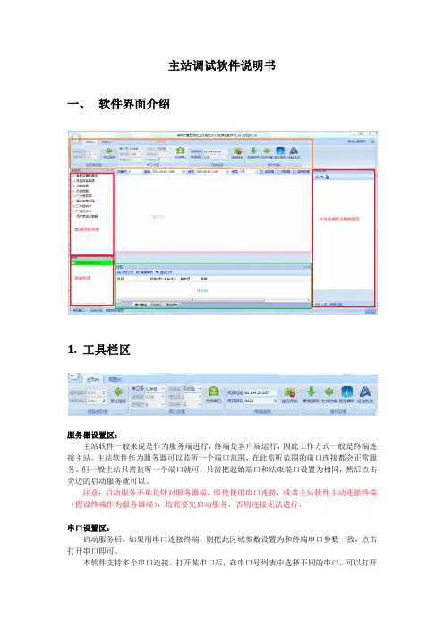
主站调试软件说明书一、软件界面介绍1.工具栏区服务器设置区：主站软件一般来说是作为服务端进行，终端是客户端运行，因此工作方式一般是终端连接主站。

主站软件作为服务器可以监听一个端口范围，在此监听范围的端口连接都会正常服务。

但一般主站只需监听一个端口就可，只需把起始端口和结束端口设置为相同，然后点击旁边的启动服务就可以。

注意：启动服务不单是针对服务器端，即使使用串口连接，或者主站软件主动连接终端（假设终端作为服务器端），均需要先启动服务，否则连接无法进行。

串口设置区：启动服务后，如果用串口连接终端，则把此区域参数设置为和终端串口参数一致，点击打开串口即可。

本软件支持多个串口连接，打开某串口后，在串口号列表中选择不同的串口，可以打开新的连接。

由于串口连接是免登陆常连接，因此打开串口后，终端列表马上显示一个新的连接，（区域码为当前串口号，终端地址为0xFFFFFF广播地址）。

终端连接区：终端连接是主站软件作为客户端来主动连接终端，设置终端IP地址和端口号后，点击右边连接终端即可。

除主动/被动工作方式不同外，其他和作为服务器端功能一致。

同时连接终端也可以连接多个，只需改变终端地址或端口号后，可以再度点击连接终端进行连接。

操作设置区：操作设置工具栏区提供了手工输入报文解释功能，支持两种格式输入，例如：68 10 00 10 00 68 5B 03 00 00 FF FF FF 01 0A 60 00 00 00 01 00 E0 A7 16，以及6810001000685B030000FFFFFF010A600000000100E0A716 ，即上述报文去掉空格。

组包发送功能是提供给用户一种和终端自主组包交互的功能，用户可以把标准规约框架之外的报文自主组包下发给终端。

由于南网规约所有数据项皆由配置而来，本软件支持规约内数据类型的任意组织，因此除非扩展了规约数据类型，且此种类型无法由现有类型配置得到，否则规约数据项的扩展是可以直接由配置生成的。

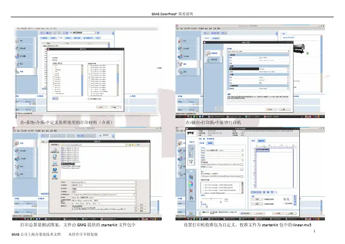
在‐系统‐介质‐中定义你所使用的打印材料（介质） 在‐输出‐打印机‐中新增打印机打印总墨量测试图案，文件由GMG提供的starterkit文件包中 设置打印机校准包为自定义，校准文件为starterkit包中的‐linear.mx3在打印机高级选项中选择打印模式，此设置在整个校准包新建过程中应一致 选中打印图像，在色彩管理选项中设置打样标准为自定义，文件为GMG软件 安装目录下profile_linear\CP_linear.mx4检查打印出的测试图，以不溢墨，线条清晰为准，选择适合的墨量 打印安装目录下TestCharts文件夹中TC4 测试图（同你的测量设备一致）在主菜单‐工具‐中打开profile editor 新建mx4文件，打印机和色域任意，选择你的测量设备，图表为TC4全色域文件，文件名例：Epsonxxxx‐720‐i1‐paper‐FullGamut.csc测量刚才打印的TC4图表（测量‐全部目标值） 测量完成后，输出目标值‐色域文件，文件名一般加上FullGamut以区分测量刚才打印的TC3图表到目标值中，另存此mx3文件打印Eci2002R 图表，打印设置同打印TC3时设置在profile editor 中新建mx4 ,打印机和色域随意，选择正确的测量色备和eci2002r 图表输出目标值为色域文件测量刚才打印的eci2002r 图表到目标值校准文件，文件名例：Epsonxxxx ‐720‐i1‐paper ‐TIL255.mx3在系统‐校准包中将校准文件和色域文件打包，注意打印机设置的一致 选择创建时的测量设备，校准文件和全色域文件定义校准公差和周期，完成后保存 打印机的校准：在输出‐打印机中选择要校准的打印机和对应的校准包在校准向导中按步骤操作，选择测量设备打印校准图表自动发送作业并打印等待干燥测量图表测量结果，如果达到要求则接受循环，如果超出标准就选择再次校准，按步骤重复闭环校准，直到Ok 。

F10 指纹读卡器软件说明书目录1.软件安装与卸载·······································································- 2 -2.设备管理 ··················································································- 5 -2.1通讯设置········································································- 8 -2.2指纹机信息····································································- 9 -2.3Wiegand ········································································- 10 -2.4验证 ············································································· - 11 -2.5电源管理······································································- 12 -2.6Mifare ············································································- 13 -2.7其他设置······································································- 13 -3.系统设置 ················································································- 28 -4.系统管理 ················································································- 29 -4.1操作员管理··································································- 29 -4.2系统操作日志 ······························································- 30 -4.3数据维护······································································- 31 -4.3.1备份数据库························································- 31 -4.3.2恢复数据库备份················································- 32 -4.3.3数据库压缩························································- 32 -4.3.4清除过期数据····················································- 32 -4.4初始化系统··································································- 33 -4.5设置数据库··································································- 34 -4.6设置数据库密码 ··························································- 35 -5.备注························································································- 36 -6.常用操作 ················································································- 39 -- 1 -1.软件安装与卸载安装软件之前建议关闭其他正在运行的应用程序，避免安装时发生冲突。

MALA GX 雷达系统
操作手册
1.0 版
北京鑫衡运公司 2014 年
目录
1 设备简介及设置 ....................................................................................1
开箱检查 ........................................................1 附件及选配件 .................................................... 1 系统装配和设置 .................................................. 3 系统连接 ........................................................4 天线 LED 指示灯 ..................................................6 电池维护和充电 .................................................. 7 GX HDR 天线电池..................................................7 用电池包（选件）给天线和控制器供电 .............................. 8 给 GX 控制器充电 .................................................8
主菜单图标
当完成雷达采集后停止和关闭系线之
11
前，它将进入电源循环模式。此时按控制器上的电源开关，等待 5-10 秒，天线 开关就会打开。如果没有这样操作，天线就不会开机。

启控组态集中监控软件用户手册2012-091.1系统概述 (1)1.2主要功能 (1)1.3系统特点 (2)第二章系统运行环境 ......................................................................................................... - 2 -第三章系统安装和启动退出 ........................................................................................... - 3 -3.1系统安装 . (3)3.2启动系统 (5)3.2.1监控系统服务器启动 (5)3.2.2客户端登入 (6)3.3退出系统 (6)第四章运行界面................................................................................................................... - 7 -4.1主页面.. (7)第五章主菜单 ....................................................................................................................... - 8 -5.1操作 (8)5.1.1注销登入 (8)5.1.2用户信息 (8)5.1.3选项 (9)5.1.4退出系统 (10)5.2视图 (10)5.2.1工程列表 (10)5.2.1.1告警上下限设置 (10)5.2.1.2事件查看 (12)5.2.1.3启动告警页面跳转 (12)5.2.1.4停止启动告警页面跳转 (12)5.3查看 (13)5.3.1历史事件查看 (13)5.3.2历史曲线查看 (13)5.3.3电话拨打记录查看 (14)5.3.4短信发送记录查看 (15)5.4告警设置 (15)5.5帮助 (16)6.1温湿度监测 (16)6.2漏水监测系统 (17)6.3UPS系统 (18)6.4空调系统 (19)6.5配电监控 (20)第七章WEB功能 ................................................................................................................ - 21 -第一章系统简介1.1系统概述随着计算机的发展和普及，计算机系统数量与日俱增，配套的环境设备也日益增多，计算机房已成为各大单位的重要组成部分。

GDGR软件安装与使用说明软件安装与使用手册GDGR无线随钻测井系统文档编号：编制部门：科研部编写：王亮审核：付翠玲发布日期：2015.09.10声明本说明的版权归斯伦贝谢金地伟业油田技术（山东）有限公司所有。

未得到本公司的书面许可，任何人不得以任何方式或形式对本手册内的任何部分进行复制、摘录、备份、修改、传播、翻译成其它语言、将其全部或部分用于商业用途。

本公司保留对本说明书及本声明的最终解释权和修改权。

本说明依据现有信息制作，其内容如有更改，恕不另行通知。

斯伦贝谢金地伟业油田技术（山东）有限公司在编写该说明书的时候已尽最大努力保证其内容准确可靠，但本公司不对本手册中的遗漏、不准确或印刷错误导致的损失和损害承担责任。

本手册所提到的软件规格和参数仅供参考，如有内容更新，恕不另行通知。

版本信息时间版本号编写人部门修改原因修改内容备注2015-8-10V1.0王亮科研部初始版本2015-9-10V2.0王亮科研部版本修改目录第一章软件运行环境要求 (1)1.1硬件配置要求 (1)1.2软件配置要求 (1)第二章GDGR软件的安装 (2)2.1SQL Server2000个人版安装 (2)2.2启动SQL server服务器 (5) 2.3GDGR系统软件的安装 (6)第三章GDGR软件的使用 (9)3.1设置 (9)3.1.1选择仪器串类型 (9)3.1.2新建测量工程 (9)3.1.3删除测量工程 (10)3.1.4设置工程参数 (11)3.1.5设置循环时间与脉冲总数 (16) 3.1.6录入钻具组合 (16)3.1.7设置开泵门槛 (18)3.1.8录入井斜记录 (19)3.2VGA司显 (22)3.3定向探管 (24)3.4伽马探管 (24)3.4.1设置伽马探管 (24)3.4.2测试伽马探管 (25)3.4.3接收存储数据 (26)3.4.4生成垂深数据 (27)3.4.5修正实时伽马测深 (28)3.4.6伽马标定系数 (30)3.4.7导入测深伽马数据 (30)3.5测量 (31)3.5.1自动测量 (31)3.5.2手动测量 (32)3.6伽马曲线 (33)3.6.1测深伽马曲线 (33)3.6.2垂深伽马曲线 (35)3.7历史数据 (38)3.7.1存储伽马数据 (38)3.7.2在线伽马数据 (39)3.7.3历史温度电压 (40)3.7.4历史全测量 (41)3.7.5历史工具面 (42)3.7.6历史钻时 (43)3.7.7原始代码数据 (44)附1-1软件操作步骤 (45)附1-2注意事项 (46)第一章软件运行环境要求1.1硬件配置要求表1-1分类最低配置推荐配置处理器主频1.0GHz以上的AMD或Intel的32位处理器主频2.0GHz以上的AMD或Intel的32/64位处理器内存1G以上内存条2G以上内存条显卡显存256MB以上的PCI-E接口显卡显存512MB以上的PCI-E接口显卡硬盘空间60GB可用硬盘空间80GB可用硬盘空间显示器分辨率在1024X768像素及以上显示器分辨率在1024X768像素及以上显示器接口串口/PCIM卡转串口串口/PCIM卡转串口1.2软件配置要求表1-2分类名称版本语种操作系统Windows xp/windows7Sp4中文/英文操作系统的附加功能无数据库平台SqlServer2000Sp4中文/英文开发平台Vc++ 6.0中文/英文客户端软件无第二章GDGR软件的安装2.1SQL Server2000个人版安装运行SQL Server2000个人版中的AUTORUN.EXE，选择安装“SQL Server 2000组件”。

如果图像质量较差，如：有条状或其他 伪影存在。在此情况下不选用该图像来分析, 点击[Exclude This Slice] 键将之去除。
图12
GEMSC CT APPL. TIP
BMD快速操作手册
7、显示BMD 的分析报告(BMD Report) 当所有的图像被分析完毕后, 点击[Show Report]
在BMD的主界面上,点击[Back up&Restore],则 进入该命令屏幕（图16）:
点击[Back up to Archive] 键，则备份BMD数据。 点击[Restore From Archive] 键，则恢复BMD数据。 点击[Check Archive Disk ]键.，则了解存盘内容。 点击Quit,则退出BMD分析系统。
一、细胞衰老
• 1、1961年，Hayflick和Moorhead报告说，培养的 人二倍体细胞表现出明显的衰老、退化和死亡的过程。 若以1：2的比率连续进行传代，则平均只能传代 40~60次，此后细胞就逐渐解体并死亡。他们的工作 表明，细胞，至少是培养的细胞，不是不死的，而是 有一定的寿命；它们的增殖能力不是无限的，而是有 一定的界限，这就是有名的Hayflick界限（Hayflick Limitation） （P460，LR17，WR12） 。
2、User Options(用户选项) 的设置
点击BMD图标（图1）,启动BMD
图1
软件,首先设置User Options（图2）,
将先前设定的扫描参数输入User
Options的图表（图3）,然后点击OK
键完成。
图3
图2
GEMSC CT APPL. TIP
BMD快速操作手册
二、扫描机的标准化(Scanner Standardization)

What do you expect to learn here?
We will illustrate some essential steps based on the sample files accompanying GMDR software, providing a quick tutorial of GMDR. Hopefully, these steps will meet your practice.
Step 7: Calculate the score
Clicking “Run”, the score will be calculated.
Step 8: Select a score
Go to Filter Tab. Select a column in the Score Table.
Step 9: Configuration
Step 5: Select a method for score calculation
Linቤተ መጻሕፍቲ ባይዱar Regression: for quantitative traits. Logistic Regression: for dichotomous traits.
Step 6: Select covariates and traits
Step 3: Do you have a Score file?
Yes, I’ve built the score (try “Score.txt”).
Clicking “Load Scorefile” button to load your score file.
Go to Step 8.
No, I can only provide covariates and traits being analyzed.

保险实训软件操作手册目录系统简介 .。

..。

.。

..。

..。

..。

..。

..。

.。

.....。

.....。

..。

...。

.。

.。

.。

.。

...。

.。

.....。

.。

.。

..。

..。

.。

.。

.。

.。

.。

.。

...。

3功能特点 .。

..。

.。

..。

..。

.。

.。

.。

.。

.。

..。

.。

..。

..。

..。

.。

.。

.。

.。

.。

...。

.。

.。

...。

.。

.。

.。

..。

...。

.。

.....。

.。

... 3业务流程 .。

.。

..。

.。

.。

....。

.。

...。

..。

....。

.。

......。

......。

.。

...。

..。

...。

....。

.。

.。

..。

...。

.。

.。

..。

.。

..。

.。

.。

.。

.. 4系统操作指南 .。

...。

.。

..。

.。

...。

.。

....。

.。

.。

.。

..。

..。

.。

.。

.。

.。

......。

.。

.。

.。

....。

..。

....。

.。

.。

.。

.... 5第一节系统界面说明。

..。

...。

....。

.。

.。

..。

.。

.。

.。

.。

...。

.。

..。

..。

.。

.。

.。

...。

.。

.。

...。

.。

.。

.。

..。

.。

...。

5λ界面组成 .....。

.。

.。

.。

.。

...。

.。

.。

.。

.。

..。

..........。

.。

..。

..。

.。

.....。

..。

.。

...。

.。

.。

..。

.. 5第二节系统登陆说明 ....。

.。

...。

.。

.。

.。

..。

..。

.。

....。

.。

.。

.。

.。

...。

...。

.。

.。

........。

..。

..。

......。

...。

.。

.。

..。

..。

.。

6λ如何登陆系统 .......。

.....。

.。

.....。

..。

..。

....。

..........。

..。

.。

...。

.。

....。

.。

...。

...。

...。

.。

6第三节财产险操作指南 . .。

.....。

.....。

.。

..。

...。

....。

.。

.。

..。

.。

.。

..。

..。

.。

.。

..。

..。

..。

MCGS工控组态软件使用说明书一、概述计算机技术和网络技术的飞速发展，为工业自动化开辟了广阔的发展空间，用户可以方便快捷地组建优质高效的监控系统，并且通过采用远程监控及诊断、双机热备等先进技术，使系统更加安全可靠，在这方面，MCGS工控组态软件将为您提供强有力的软件支持。

MCGS工控组态软件是一套32位工控组态软件，可稳定运行于Windows95/98/NT操作系统，集动画显示、流程控制、数据采集、设备控制与输出、网络数据传输、双机热备、工程报表、数据与曲线等诸多强大功能于一身，并支持国内外众多数据采集与输出设备。

二、软件组成(一)按使用环境分，MCGS组态软件由“MCGS组态环境”和“MCGS运行环境”两个系统组成。

两部分互相独立，又紧密相关，分述如下：1.MCGS组态环境：该环境是生成用户应用系统的工作环境，用户在MCGS组态环境中完成动画设计、设备连接、编写控制流程、编制工程打印报表等全部组态工作后，生成扩展名为.mcg的工程文件，又称为组态结果数据库，其与MCGS 运行环境一起，构成了用户应用系统，统称为“工程”。

2.MCGS运行环境：该环境是用户应用系统的运行环境，在运行环境中完成对工程的控制工作。

(二)按组成要素分，MCGS工程由主控窗口、设备窗口、用户窗口、实时数据库和运行策略五部分构成：1.主控窗口：是工程的主窗口或主框架。

在主控窗口中可以放置一个设备窗口和多个用户窗口，负责调度和管理这些窗口的打开或关闭。

主要的组态操作包括：定义工程的名称，编制工程菜单，设计封面图形，确定自动启动的窗口，设定动画刷新周期，指定数据库存盘文件名称及存盘时间等。

2.设备窗口：是连接和驱动外部设备的工作环境。

在本窗口内配置数据采集与控制输出设备，注册设备驱动程序，定义连接与驱动设备用的数据变量。

3.用户窗口：本窗口主要用于设置工程中人机交互的界面，诸如：生成各种动画显示画面、报警输出、数据与曲线图表等。

背景图片：如果此分区有背景图片时可以指定，背景图片一般包括楼层图、区域图等。
背景颜色：背景颜色，指定此分区的背景颜色，可以使设备图标和背景的对比度增强，增强视觉效果。
分区信息定义完成后，点击“确定”按钮，系统会把分区添加到监控工程列表项，如图15所示。
图15分区列表
所定义的分区背景图、背景颜色信息都会在界面上呈现。
1、用鼠标单击任务栏上面的时间，弹出时间窗口，如图6所示。点击 按钮，出现编辑按钮。
图6时间窗口
2、点击 按钮，弹出时钟首选项窗口，如图7所示。
图7时钟首选项
3、在时钟首选项窗口中点击 按钮，弹出时间和日期设置窗口，如图8所示。
图8时间和日期
4、修改时间为当前本地的时间后，点击 按钮，即可。
5、有时要求认证，将弹出如图9所示的认证窗口。请在密码框中输入安装软件时创建的用户密码即可。
控制器：控制器ID，可以通过设置这一项选择工程中不同的控制器。
回路：相应控制器中的回路号。
分区：相应控制器中的分区号。
通过对控制器、回路、分区三项的不同选择，可以对设备进行过滤，便于用户更好的选择需要的设备。
图18设备列表
6.4.6.3
6.4.6.4
1)选定要对齐的设备
2)
点击鼠标左键，按住不放拖动，当所有要对齐的设备都已经包含在鼠标托动的矩形框中时放开鼠标左键，这样要对齐的设备就都已经选定，且都有选择框包围，如图19所示。
图24工程文件拷贝路径
在任务栏上点击位置菜单，选择计算机，指点打开文件系统，再打开opt文件夹，再打开gm9000文件夹，接着打开Project文件夹即可。
第7章
第8章
8.1
8.2
火灾报警监控图形显示系统是整个消防监控系统图形监控中心，用户能够直观地了解工程设备布置情况，当设备发生异常信息，例如火警、故障、动作等信息时，能够使用户最快、最直观地掌握事件发生的位置信息，主界面如图25所示。

温度控制仪器软件使用说明温度控制仪器软件无需安装，将光盘中“温度控制仪器软件.exe”软件直接复制到你计算机即可。

双击打开“温度控制仪器软件”，出现如下图1-1界面。

图1-1界面上部为菜单栏，由“通讯设置”，“曲线设置”、“历史记录”、“打印”、“退出”等选项组成。

运行时，先点击菜单栏“通讯设置”进行通讯设置。

点击“通讯设置”——“设置参数”后，出现图1-2界面：图1-2 通讯设置界面在图1-2界面中的“端口号”框里写如计算机的串口端口号，在“地址号”的框里写入仪表的Addr值,“波特率”框里写入bAud的值(注：一般设置Addr 值为1，bAud为9600)。

设置好上述3个选项后，按“确认”按钮继续。

如果通讯连接不正确，将出现如图1-3“通讯未连接”的提示界面图1-3如果通讯连接正常，软件左边的仪表参数将出现读入的参数值，如图1-4所示：图1-4图1-4中读入的各个值就是仪表的当前参数值。

这里大多数数值都可以进行修改。

修改时，可以在“确认修改”前面的方框里写入要修改的数值，然后按“确认修改按钮即可。

在方框后面有下拉框的地方，点击下拉框，选中将修改的选项即可。

设置完成后，点击菜单栏中的“曲线设置”——“曲线参数设置”，当所做实验为温度实验时，将出现图1-5界面：图1-5所做实验不是温度实验时，出现界面如图1-6所示：图1-7输出最大值、输出最小值、输入最大值与输入最小值将决定曲线的范围，默认设置是根据仪表的设置而来，用户可以根据自己需要自行修改。

“采样间隔”设置的是2次采样之间的时间间隔，最小时间为300mS.设置好之后按“OK”按钮即完成设置。

此时界面中的“操作框”先面显示出了设定参数，如图1-8所示：图1-8点击图1-8的“开始采集”开始采集信号，同时实验曲线自动绘制，实验数据同时也显示下面表格中，分别如图1-9和图1-10所示：图1-9图1-10实验完成后，点击图1-8中的“结束采集”按钮。

GMG操作流程一、软件简介1.软件组成(1） GMG Colorproof打印机配置，使用校准向导校准打印机，手动开始一个作业和热文件夹安装.(2) GMG 色彩管理文件编辑器创建和编辑mx3， mx4 色彩管理文件测试图表的测量方法。

mx3 文件是校准文件，而mx4 文件描述的是特殊装置的特性.(3) GMG 专色编辑器创建和编辑专色数据库。

(4) GMG Rip 服务器Colorproof 一样支持PS、PDF、EPS文件。

2.软件的结构文件（1) 打印机校准文件＊.mx3mx3 文件是一个用于校准颜色的三维色彩管理文件.它为印刷设备定义了特殊的媒介/油墨的结合。

如果打印机属性出现了偏差，该定义好的色彩标准可以让您再次校准使用GMG Colorproof 的打印机,因此，您可以稳定重复的得到色彩准确的样张。

（2) 全范围文件（Gamut File）＊.csc一个全范围文件描述了一台打印机的最大色彩容量。

当从对象值计算和从目标和当前设备值计算时需要全范围文件.有两种不同类型的全范围文件：用于mx4 彩色profile 文件的“一般”全范围文件和用于打印机校准和特殊色彩的色彩管理文件的“完全全范围”文件.全范围文件描述了打印机的整个的、无限制的色域空间,其能够满足打印机校准的需求.用于打印机校准的简化色域空间常用于计算一个mx4/mx5 的色彩管理文件。

(3) 彩色色彩管理文件*.mx4这是一个用于从CMYK 到CMYK 转换的四维与设备相关的色彩管理文件。

当打印连续调样张(用于印刷机的非模拟网点图案的色彩匹配样张）时使用该文件。

该色彩管理文件使用纸张、油墨和根据目标值校准的印刷机的特定组合（如胶印)模拟打样，描述打样机的输出特性.（4）模板文件＊.tpl模板文件是一个关于几何、排列以及为特殊的测量装置而配置的带有测试图表的色彩图解的记录文件.(5) 控制条文件＊。

tif, *.gmg控制条是TIFF 文件格式(二值和连续）的印刷工艺控制条，它可以随样张一起被打印出来。

提示 ：当储存卡空间不足，数据灯（状态红灯）快闪，并将停止记录数据。现有的数据文件不会被覆盖。
RTK数据存储
iHand 10手簿和GIS+手簿都可以通过蓝牙或电缆线连接中海达V30接收机，当设置完成开始工作以后，采集到的RTK数据存储在手簿的存储卡里，可通过随机配置的手簿数据线将RTK数据下载到您的电脑上。
腐蚀性液体或气体
电子干扰源
请勿将GNSS接收机安置在电力及具有强干扰信号的污染源附近，比如：
油道（火花塞）
电视及电脑显示器
发电机
电动摩托
直流-交流电源转换设备
荧光灯
电源开关
CHAPTER
4
基本操作
本章节介绍：
■引言
■按键功能
■指示灯说明
■启动和停止接收机
■静态数据存储
■RTK数据存储
■复位接收机
■恢复出厂设置
喇叭：仪器实时操作及状态进行语音播报。
提示：1、工作中暂时不需要使用五芯插座、八芯插座和差分天线接口时请盖上胶塞，达到防水防尘的目的。
2、当喇叭进水时，可能出现喇叭无声或声音沙哑，待烘干后声音将恢复正常。
通信
如图3-5，为通信模块外观图，V30接收机可根据不同需求安装传统UHF电台、GPRS和3G通信模块。
方式
卫星灯（单绿灯）
信号灯（双灯之绿灯）
基准站
●
○
移动站
○
●
静态
●
●
2、数据链(双击F2进入数据链设置模式，之后再单击F2进行模式选择，按电源键确认，超过十秒未按电源键，将自动确认)：●亮○灭
类型
卫星灯（单绿灯）
信号灯（双灯之绿灯）
UHF/GSM/CMDA
●