
DCT压缩解压压缩比PSNR计算MATLAB源代码
- 格式:doc
- 大小:12.00 KB
- 文档页数:2



本科毕业设计论文题目:基于DCT变换的图像压缩技术的研究专业名称:学生姓名:指导教师:毕业时间:毕业一、题目基于DCT变换的图像压缩技术的研究二、指导思想和目的要求指导思想:图像信息给人们以直观、生动的形象,成为人们获取外部信息的重要途径。
然而数字图像具有极大的数据量。
在目前的计算机系统条件下,若图像信息不经过压缩,则会占用信道,传输速率变慢,而且传输成本变得昂贵,这对图像的储存、传输及使用都非常不利,同时也阻碍了人们对图像的有效获取和使用。
因此,图像压缩技术的重要性也越来越高,在学习、生产、生活等方面的作用也越来越显著,对图像进行压缩成为图像研究领域的重要课题。
目的要求:基于DCT变换的图像压缩技术,首先介绍图像压缩的基本原理及方法,然后了解离散余弦变换的性质以及JPEG图像压缩算法,最后从DCT 变换、量化以及熵编码三个过程进行详细论述,利用MATLAB仿真软件实现基于DCT变换的图像压缩,去除冗余数据,节约文件所占的码字,降低原始图像数据量,解决图像数据量巨大的问题,以达到对图像进行压缩的目的。
三、主要技术指标图像的质量评价方法主要有两种:一种是主观评价,另一种是客观评价。
主观评价直接反映人眼的视觉感受,主要从亮度、色调、饱和度和细节分辨等方面入手,但因观察者个体差异、人力成本较高等原因而存在许多不足之处。
通常客观评价的方法应用更广泛。
常用的客观评价方法和标准有压缩比(CR)和峰值信噪比(PSNR)两种。
再根据不同的量化系数得到不同的压缩比和峰值信噪比。
x,和标准图像f0()y x,的大小是M⨯N,常用客观评价指标定设待评价图像f()y义如下:x,/f0()y x,不同的量化系数压缩比也不同(量化系数分压缩比:r=f()y别为:1、3、5、10、15等)由于量化系数不同得到的峰值信噪比也不同,根据均方差得出峰值信噪比。
均方差: MSE =()[]()[]}{()[]∑∑∑∑-=-=-=-=-10102010x 10y 20,,,M x N y M N y x f y x f Q y x f Q 式中,运算符Q []∙表示在计算前,为使计算值与人眼视觉感受一致而进行的某种预处理,如对数处理、幂处理等。
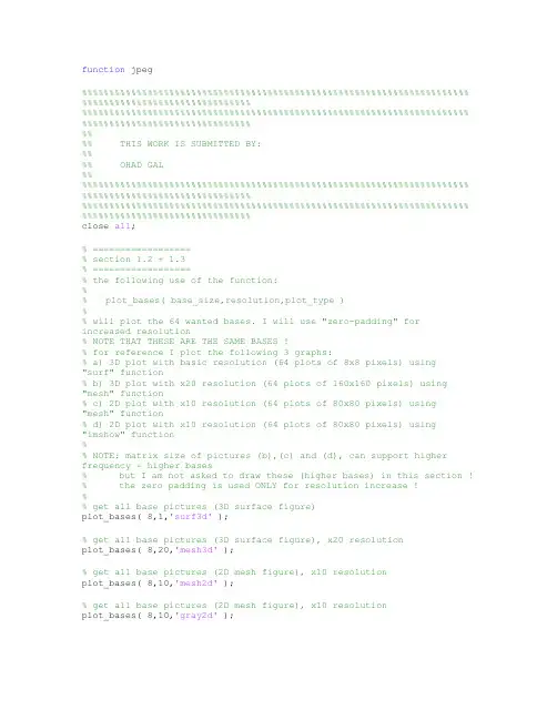
function jpeg %%%%%%%%%%%%%%%%%%%%%%%%%%%%%%%%%%%%%%%%%%%%%%%%%%%%%%%%%%%%%%%%%%%%%%% %%%%%%%%%%%%%%%%%%%%%%%%%%%%%%% %%%%%%%%%%%%%%%%%%%%%%%%%%%%%%%%%%%%%%%%%%%%%%%%%%%%%%%%%%%%%%%%%%%%%%% %%%%%%%%%%%%%%%%%%%%%%%%%%%%%%%%%%% THIS WORK IS SUBMITTED BY:%%%% OHAD GAL%% %%%%%%%%%%%%%%%%%%%%%%%%%%%%%%%%%%%%%%%%%%%%%%%%%%%%%%%%%%%%%%%%%%%%%%% %%%%%%%%%%%%%%%%%%%%%%%%%%%%%%% %%%%%%%%%%%%%%%%%%%%%%%%%%%%%%%%%%%%%%%%%%%%%%%%%%%%%%%%%%%%%%%%%%%%%%% %%%%%%%%%%%%%%%%%%%%%%%%%%%%%%%close all;% ==================% section 1.2 + 1.3% ==================% the following use of the function:%% plot_bases( base_size,resolution,plot_type )%% will plot the 64 wanted bases. I will use "zero-padding" forincreased resolution% NOTE THAT THESE ARE THE SAME BASES !% for reference I plot the following 3 graphs:% a) 3D plot with basic resolution (64 plots of 8x8 pixels) using "surf" function% b) 3D plot with x20 resolution (64 plots of 160x160 pixels) using "mesh" function% c) 2D plot with x10 resolution (64 plots of 80x80 pixels) using "mesh" function% d) 2D plot with x10 resolution (64 plots of 80x80 pixels) using "imshow" function%% NOTE: matrix size of pictures (b),(c) and (d), can support higher frequency = higher bases% but I am not asked to draw these (higher bases) in this section ! % the zero padding is used ONLY for resolution increase !%% get all base pictures (3D surface figure)plot_bases( 8,1,'surf3d' );% get all base pictures (3D surface figure), x20 resolutionplot_bases( 8,20,'mesh3d' );% get all base pictures (2D mesh figure), x10 resolutionplot_bases( 8,10,'mesh2d' );% get all base pictures (2D mesh figure), x10 resolutionplot_bases( 8,10,'gray2d' );% ==================% section 1.4 + 1.5% ==================% for each picture {'0'..'9'} perform a 2 dimensional dct on 8x8 blocks.% save the dct inside a cell of the size: 10 cells of 128x128 matrix% show for each picture, it's dct 8x8 block transform.for idx = 0:9% load a pictureswitch idxcase {0,1}, input_image_128x128 =im2double( imread( sprintf( '%d.tif',idx ),'tiff' ) );otherwise, input_image_128x128 =im2double( imread( sprintf( '%d.tif',idx),'jpeg' ) );end% perform DCT in 2 dimension over blocks of 8x8 in the given picture dct_8x8_image_of_128x128{idx+1} =image_8x8_block_dct( input_image_128x128 );if (mod(idx,2)==0)figure;endsubplot(2,2,mod(idx,2)*2+1);imshow(input_image_128x128);title( sprintf('image #%d',idx) );subplot(2,2,mod(idx,2)*2+2);imshow(dct_8x8_image_of_128x128{idx+1});title( sprintf('8x8 DCT of image #%d',idx) );end% ==================% section 1.6% ==================% do statistics on the cell array of the dct transforms% create a matrix of 8x8 that will describe the value of each "dct-base"% over the transform of the 10 given pictures. since some of the values are% negative, and we are interested in the energy of the coefficients, we will% add the abs()^2 values into the matrix.% this is consistent with the definition of the "Parseval relation" in Fourier Coefficients% initialize the "average" matrixmean_matrix_8x8 = zeros( 8,8 );% loop over all the picturesfor idx = 1:10% in each picture loop over 8x8 elements (128x128 = 256 * 8x8 elements)for m = 0:15for n = 0:15mean_matrix_8x8 = mean_matrix_8x8 + ...abs( dct_8x8_image_of_128x128{idx}(m*8+[1:8],n*8+[1:8]) ).^2;endendend% transpose the matrix since the order of the matrix is elements along the columns,% while in the subplot function the order is of elements along the rows mean_matrix_8x8_transposed = mean_matrix_8x8';% make the mean matrix (8x8) into a vector (64x1)mean_vector = mean_matrix_8x8_transposed(:);% sort the vector (from small to big)[sorted_mean_vector,original_indices] = sort( mean_vector );% reverse order (from big to small)sorted_mean_vector = sorted_mean_vector(end:-1:1);original_indices = original_indices(end:-1:1);% plot the corresponding matrix as asked in section 1.6figure;for idx = 1:64subplot(8,8,original_indices(idx));axis off;h = text(0,0,sprintf('%4d',idx));set(h,'FontWeight','bold');text(0,0,sprintf('\n_{%1.1fdb}',20*log10(sorted_mean_vector(idx)) ));end% add a title to the figuresubplot(8,8,4);h = title( 'Power of DCT coefficients (section 1.6)' );set( h,'FontWeight','bold' );% ==================% section 1.8% ==================% picture 8 is chosen% In this section I will calculate the SNR of a compressed image againts% the level of compression. the SNR calculation is defined in the header% of the function: <<calc_snr>> which is given below.%% if we decide to take 10 coefficients with the most energy, we will% zeros to the other coefficients and remain with a vector 64 elements long% (or a matrix of 8x8)% load the original imageoriginal_image = im2double( imread( '8.tif','jpeg' ) );% I will use this matrix to choose only the wanted number ofcoefficients% the matrix is initialized to zeros -> don't choose any coefficient at allcoef_selection_matrix = zeros(8,8);% compressed picture set (to show the degrading)compressed_set = [1 3 5 10 15 20 30 40];% this loop will choose each time, the "next-most-energetic"coefficient,% to be added to the compressed image -> and thus to improove the SNRfor number_of_coefficient = 1:64% find the most energetic coefficient from the mean_matrix[y,x] = find(mean_matrix_8x8==max(max(mean_matrix_8x8)));% select if for the compressed imagecoef_selection_matrix(y,x) = 1;% replicate the selection matrix for all the parts of the dct transform% (remember that the DCT transform creates a set of 8x8 matrices, where% in each matrix I need to choose the coefficients defined by the % <<coef_selection_matrix>> matrix )selection_matrix = repmat( coef_selection_matrix,16,16 );% set it as zero in the mean_matrix, so that in the next loop, we will% choose the "next-most-energetic" coefficientmean_matrix_8x8(y,x) = 0;% choose the most energetic coefficients from the original image% (total of <<number_of_coefficient>> coefficients for this run in the loop)compressed_image = image_8x8_block_dct(original_image) .*selection_matrix;% restore the compressed image from the given set of coeficientsrestored_image = image_8x8_block_inv_dct( compressed_image );% calculate the snr of this image (based on the original image)SNR(number_of_coefficient) =calc_snr( original_image,restored_image );if ~isempty(find(number_of_coefficient==compressed_set))if (number_of_coefficient==1)figure;subplot(3,3,1);imshow( original_image );title( 'original image' );endsubplot(3,3,find(number_of_coefficient==compressed_set)+1);imshow( restored_image );title( sprintf('restored image with %dcoeffs',number_of_coefficient) );endend% plot the SNR graphfigure;plot( [1:64],20*log10(SNR) );xlabel( 'numer of coefficients taken for compression' );ylabel( 'SNR [db] ( 20*log10(.) )' );title( 'SNR graph for picture number 8, section 1.8' );grid on; %%%%%%%%%%%%%%%%%%%%%%%%%%%%%%%%%%%%%%%%%%%%%%%%%%%%%%%%%%%%%%%%%%%%%%% %%%%%%%%%%%%%% --------------------------------------------------------------------------------%% I N N E R F U N C T I O N I M P L E M E N T A T I O N%% --------------------------------------------------------------------------------%%%%%%%%%%%%%%%%%%%%%%%%%%%%%%%%%%%%%%%%%%%%%%%%%%%%%%%%%%%%%%%%%%%%%%% %%%%%%%%%%%%% ---------------------------------------------------------------------------------% pdip_dct2 - implementation of a 2 Dimensional DCT%% assumption: input matrix is a square matrix !% ---------------------------------------------------------------------------------function out = pdip_dct2( in )% get input matrix sizeN = size(in,1);% build the matrixn = 0:N-1;for k = 0:N-1if (k>0)C(k+1,n+1) = cos(pi*(2*n+1)*k/2/N)/sqrt(N)*sqrt(2);elseC(k+1,n+1) = cos(pi*(2*n+1)*k/2/N)/sqrt(N);endendout = C*in*(C');% ---------------------------------------------------------------------------------% pdip_inv_dct2 - implementation of an inverse 2 Dimensional DCT%% assumption: input matrix is a square matrix !% ---------------------------------------------------------------------------------function out = pdip_inv_dct2( in )% get input matrix sizeN = size(in,1);% build the matrixn = 0:N-1;for k = 0:N-1if (k>0)C(k+1,n+1) = cos(pi*(2*n+1)*k/2/N)/sqrt(N)*sqrt(2);elseC(k+1,n+1) = cos(pi*(2*n+1)*k/2/N)/sqrt(N);endendout = (C')*in*C;% ---------------------------------------------------------------------------------% plot_bases - use the inverse DCT in 2 dimensions to plot the base pictures%% Note: we can get resolution be zero pading of the input matrix% that is by calling: in = zeros(base_size*resolution)% where: resolution is an integer > 1% So I will use zero pading for resolution (same as in the fourier theory)% instead of linear interpolation.% ---------------------------------------------------------------------------------function plot_bases( base_size,resolution,plot_type )figure;for k = 1:base_sizefor l = 1:base_sizein = zeros(base_size*resolution);in(k,l) = 1; % "ask" for the "base-harmonic (k,l)"subplot( base_size,base_size,(k-1)*base_size+l );switch lower(plot_type)case'surf3d', surf( pdip_inv_dct2( in ) );case'mesh3d', mesh( pdip_inv_dct2( in ) );case'mesh2d', mesh( pdip_inv_dct2( in ) ); view(0,90);case'gray2d', imshow( 256*pdip_inv_dct2( in ) );endaxis off;end% add a title to the figuresubplot(base_size,base_size,round(base_size/2));h = title( 'Bases of the DCT transform (section 1.3)' );set( h,'FontWeight','bold' );% ---------------------------------------------------------------------------------% image_8x8_block_dct - perform a block DCT for an image% ---------------------------------------------------------------------------------function transform_image = image_8x8_block_dct( input_image )transform_image = zeros( size( input_image,1 ),size( input_image,2 ) ); for m = 0:15for n = 0:15transform_image( m*8+[1:8],n*8+[1:8] ) = ...pdip_dct2( input_image( m*8+[1:8],n*8+[1:8] ) );endend% ---------------------------------------------------------------------------------% image_8x8_block_inv_dct - perform a block inverse DCT for an image% ---------------------------------------------------------------------------------function restored_image = image_8x8_block_inv_dct( transform_image ) restored_image =zeros( size( transform_image,1 ),size( transform_image,2 ) );for m = 0:15for n = 0:15restored_image( m*8+[1:8],n*8+[1:8] ) = ...pdip_inv_dct2( transform_image( m*8+[1:8],n*8+[1:8] ) );endend% ---------------------------------------------------------------------------------% calc_snr - calculates the snr of a figure being compressed%% assumption: SNR calculation is done in the following manner:% the deviation from the original image is considered% to be the noise therefore:%% noise = original_image - compressed_image%% the SNR is defined as:%% SNR = energy_of_image/energy_of_noise%% which yields:% SNR = energy_of_image/((original_image-compressed_image)^2)% ---------------------------------------------------------------------------------function SNR = calc_snr( original_image,noisy_image )original_image_energy = sum( original_image(:).^2 );noise_energy = sum( (original_image(:)-noisy_image(:)).^2 );SNR = original_image_energy/noise_energy;以下是1-9号原图像,放到matlab的.m文件目录里,重命名9个图像名为1、2、3、4、5、6、7、8、9。

MATLAB中常见的视频压缩算法介绍随着数字视频技术的不断发展,视频压缩算法成为了一项重要的研究领域。
在视频传输、存储和处理等应用中,压缩算法可以显著减少数据量和带宽要求,提高传输效率和存储容量。
在MATLAB中,有许多常见的视频压缩算法可以应用于多种视频处理任务。
在本篇文章中,我们将介绍一些常见的MATLAB视频压缩算法,涉及到有损压缩和无损压缩等不同类型的算法。
1. 背景介绍视频压缩算法的研究始于上世纪70年代末期,随着计算机性能的提升和通信技术的进步,视频压缩算法得到了长足的发展。
视频压缩可以分为有损压缩和无损压缩两个主要的类型。
有损压缩算法基于人类视觉系统的特性,通过舍弃一些不重要的信息以降低数据量。
而无损压缩算法则是保留了所有原始数据,但通过一系列编码技术来减小数据规模。
2. 常见的视频压缩算法2.1 MPEG算法MPEG(Moving Picture Experts Group)是一系列视频压缩标准的简称。
其中,最常用的是MPEG-2和MPEG-4。
MPEG-2主要用于广播电视等领域,而MPEG-4则适用于多媒体通信和互联网应用。
这些算法利用运动估计、离散余弦变换和熵编码等技术,通过压缩关键帧和运动补偿来实现高效的视频压缩。
2.2 H.264算法H.264(也称为AVC,Advanced Video Coding)是一种广泛应用于视频压缩的标准。
与MPEG算法相比,H.264在保持高质量视频的同时实现了更高的压缩率。
H.264算法引入了预测编码、变换编码和熵编码等一系列技术,使得视频压缩效果更加出色。
2.3 VP9算法VP9是由Google开发的一种开放源代码视频编解码器。
它是WebM媒体格式的基础,主要用于在线视频的压缩和传输。
VP9算法采用了基于块的变换编码和自适应量化等技术,以提供更高的压缩性能。
3. MATLAB中的视频压缩实现在MATLAB中,可以利用视频处理工具箱提供的函数和工具来实现视频压缩算法。