稳态热分析报告案例(ANSYS15.0版)
- 格式:doc
- 大小:140.72 KB
- 文档页数:11
第1篇一、实验目的本实验旨在通过仿真软件对某电子设备进行热分析,了解设备在正常工作状态下的温度分布,分析设备的散热性能,为设备的结构优化和热设计提供理论依据。
二、实验背景随着电子技术的不断发展,电子设备的功能和复杂程度不断提高,集成度也越来越高。
然而,电子设备单位体积的功耗不断增大,导致设备温度迅速上升,从而引起设备故障。
因此,对电子设备进行热分析,优化散热设计,对于提高设备的可靠性和使用寿命具有重要意义。
三、实验方法1. 选择仿真软件:本实验选用Ansys Fluent软件进行热分析。
2. 建立模型:根据实际设备结构,在CAD软件中建立三维模型,并将其导入Ansys Fluent中进行网格划分。
3. 定义材料属性:设置模型的材料属性,包括热导率、比热容、密度等。
4. 设置边界条件:根据设备的工作环境,设置边界条件,如环境温度、热流密度等。
5. 定义求解器:选择适当的求解器,如稳态热传导、瞬态热传导等。
6. 运行仿真:启动仿真计算,获取设备在正常工作状态下的温度分布。
7. 分析结果:对仿真结果进行分析,评估设备的散热性能。
四、实验结果与分析1. 温度分布通过仿真计算,得到设备在正常工作状态下的温度分布如图1所示。
由图可知,设备的热量主要集中在散热器附近,温度最高点约为80℃,远低于设备的最高工作温度。
2. 散热性能从仿真结果可以看出,设备散热性能良好,主要表现在以下几个方面:(1)温度分布均匀:设备内部温度分布较为均匀,没有出现明显的热点区域。
(2)散热器效果显著:散热器可以有效降低设备温度,提高设备散热性能。
(3)环境温度影响较小:在环境温度较高的情况下,设备温度升高幅度较小。
3. 优化建议根据仿真结果,提出以下优化建议:(1)优化散热器设计:考虑采用更大面积的散热器,提高散热效率。
(2)改进结构设计:优化设备内部结构,提高散热通道的流通性。
(3)采用新型散热材料:研究新型散热材料,降低设备的热阻。


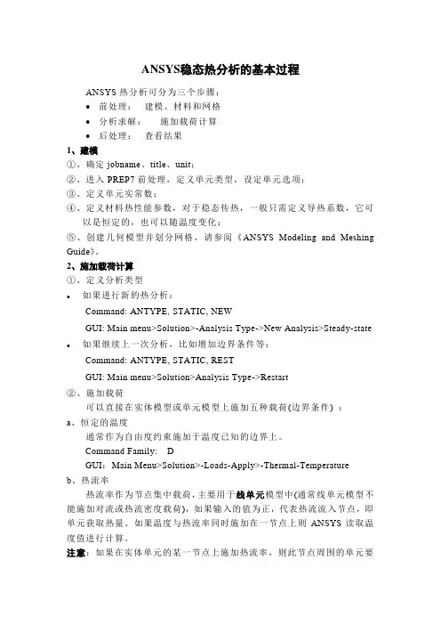
ANSYS稳态热分析的基本过程ANSYS热分析可分为三个步骤:•前处理:建模、材料和网格•分析求解:施加载荷计算•后处理:查看结果1、建模①、确定jobname、title、unit;②、进入PREP7前处理,定义单元类型,设定单元选项;③、定义单元实常数;④、定义材料热性能参数,对于稳态传热,一般只需定义导热系数,它可以是恒定的,也可以随温度变化;⑤、创建几何模型并划分网格,请参阅《ANSYS Modeling and Meshing Guide》。
2、施加载荷计算①、定义分析类型●如果进行新的热分析:Command: ANTYPE, STATIC, NEWGUI: Main menu>Solution>-Analysis Type->New Analysis>Steady-state●如果继续上一次分析,比如增加边界条件等:Command: ANTYPE, STATIC, RESTGUI: Main menu>Solution>Analysis Type->Restart②、施加载荷可以直接在实体模型或单元模型上施加五种载荷(边界条件) :a、恒定的温度通常作为自由度约束施加于温度已知的边界上。
Command Family: DGUI:Main Menu>Solution>-Loads-Apply>-Thermal-Temperatureb、热流率热流率作为节点集中载荷,主要用于线单元模型中(通常线单元模型不能施加对流或热流密度载荷),如果输入的值为正,代表热流流入节点,即单元获取热量。
如果温度与热流率同时施加在一节点上则ANSYS读取温度值进行计算。
注意:如果在实体单元的某一节点上施加热流率,则此节点周围的单元要密一些,在两种导热系数差别很大的两个单元的公共节点上施加热流率时,尤其要注意。
此外,尽可能使用热生成或热流密度边界条件,这样结果会更精确些。

ANSYS热分析指南(第三章)第三章稳态热分析3.1稳态传热的定义ANSYS/Multiphysics,ANSYS/Mechanical,ANSYS/FLOTRAN和ANSYS/Professional这些产品支持稳态热分析。
稳态传热用于分析稳定的热载荷对系统或部件的影响。
通常在进行瞬态热分析以前,进行稳态热分析用于确定初始温度分布。
也可以在所有瞬态效应消失后,将稳态热分析作为瞬态热分析的最后一步进行分析。
稳态热分析可以计算确定由于不随时间变化的热载荷引起的温度、热梯度、热流率、热流密度等参数。
这些热载荷包括:对流辐射热流率热流密度(单位面积热流)热生成率(单位体积热流)固定温度的边界条件稳态热分析可用于材料属性固定不变的线性问题和材料性质随温度变化的非线性问题。
事实上,大多数材料的热性能都随温度变化,因此在通常情况下,热分析都是非线性的。
当然,如果在分析中考虑辐射,则分析也是非线性的。
3.2热分析的单元ANSYS和ANSYS/Professional中大约有40种单元有助于进行稳态分析。
有关单元的详细描述请参考《ANSYS Element Reference》,该手册以单元编号来讲述单元,第一个单元是LINK1。
单元名采用大写,所有的单元都可用于稳态和瞬态热分析。
其中SOLID70单元还具有补偿在恒定速度场下由于传质导致的热流的功能。
这些热分析单元如下:表3-1二维实体单元表3-2三维实体单元表3-3辐射连接单元表3-4传导杆单元表3-5对流连接单元表3-6壳单元表3-7耦合场单元表3-8特殊单元3.3热分析的基本过程ANSYS热分析包含如下三个主要步骤:前处理:建模求解:施加荷载并求解后处理:查看结果以下的内容将讲述如何执行上面的步骤。
首先,对每一步的任务进行总体的介绍,然后通过一个管接处的稳态热分析的实例来引导读者如何按照GUI路径逐步完成一个稳态热分析。
最后,本章提供了该实例等效的命令流文件。

A N S Y S热分析指南——A N S Y S稳态热分析ANSYS热分析指南(第三章)第三章稳态热分析3.1稳态传热的定义ANSYS/Multiphysics,ANSYS/Mechanical,ANSYS/FLOTRAN和ANSYS/Professional这些产品支持稳态热分析。
稳态传热用于分析稳定的热载荷对系统或部件的影响。
通常在进行瞬态热分析以前,进行稳态热分析用于确定初始温度分布。
也可以在所有瞬态效应消失后,将稳态热分析作为瞬态热分析的最后一步进行分析。
稳态热分析可以计算确定由于不随时间变化的热载荷引起的温度、热梯度、热流率、热流密度等参数。
这些热载荷包括:对流辐射热流率热流密度(单位面积热流)热生成率(单位体积热流)固定温度的边界条件稳态热分析可用于材料属性固定不变的线性问题和材料性质随温度变化的非线性问题。
事实上,大多数材料的热性能都随温度变化,因此在通常情况下,热分析都是非线性的。
当然,如果在分析中考虑辐射,则分析也是非线性的。
3.2热分析的单元ANSYS和ANSYS/Professional中大约有40种单元有助于进行稳态分析。
有关单元的详细描述请参考《ANSYS Element Reference》,该手册以单元编号来讲述单元,第一个单元是LINK1。
单元名采用大写,所有的单元都可用于稳态和瞬态热分析。
其中SOLID70单元还具有补偿在恒定速度场下由于传质导致的热流的功能。
这些热分析单元如下:表3-1二维实体单元表3-2三维实体单元表3-3辐射连接单元表3-4传导杆单元表3-5对流连接单元表3-6壳单元表3-7耦合场单元表3-8特殊单元3.3热分析的基本过程ANSYS热分析包含如下三个主要步骤:前处理:建模求解:施加荷载并求解后处理:查看结果以下的内容将讲述如何执行上面的步骤。
首先,对每一步的任务进行总体的介绍,然后通过一个管接处的稳态热分析的实例来引导读者如何按照GUI路径逐步完成一个稳态热分析。
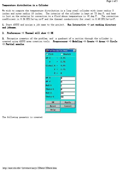
Temperature distribution in a CylinderWe wish to compute the temperature distribution in a long steel cylinder with inner radius 5 inches and outer radius 10 inches. The interior of the cylinder is kept at 75 deg F, and heatis lost on the exterior by convection to a fluid whose temperature is 40 deg F. The convection coefficient is 0.56 BTU/hr-sq.in-F and the thermal conductivity for steel is 0.69 BTU/hr-in-F.1. Start ANSYS and assign a job name to the project. Run Interactive -> set working directory and jobname.2. Preferences -> Thermal will show -> OK3. Recognize symmetry of the problem, and a quadrant of a section through the cylinder is created using ANSYS area creation tools. Preprocessor -> Modeling -> Create -> Areas -> Circle -> Partial annulusThe following geometry is created.4. Preprocessor -> Element Type -> Add/Edit/Delete -> Add -> Thermal Solid -> Solid 8 node 77 -> OK -> Close5. Preprocessor -> Material Props -> Isotropic -> Material Number 1 -> OKEX = 3.E7 (psi)DENS = 7.36E-4 (lb sec^2/in^4)ALPHAX = 6.5E-6PRXY = 0.3KXX = 0.69 (BTU/hr-in-F)6. Mesh the area and refine using methods discussed in previous examples.7. Preprocessor -> Loads -> Apply -> Temperatures -> NodesSelect the nodes on the interior and set the temperature to 75.8. Preprocessor -> Loads -> Apply -> Convection -> LinesSelect the lines defining the outer surface and set the convection coefficient to 0.56 and the fluid temp to 40.9. Preprocessor -> Loads -> Apply -> Heat Flux -> LinesTo account for symmetry, select the vertical and horizontal lines of symmetry and set the heat flux to zero.10. Solution -> Solve current LS11. General Postprocessor -> Plot Results -> Nodal Solution -> TemperaturesThe temperature on the interior is 75 F and on the outside wall it is found to be 45. These results can be checked using results from heat transfer theory.BackThermal Stress of a Cylinder using Axisymmetric ElementsA steel cylinder with inner radius 5 inches and outer radius 10 inches is 40 inches long and has spherical end caps. The interior of the cylinder is kept at 75 deg F, and heat is lost on the exterior by convection to a fluid whose temperature is 40 deg F. The convection coefficient is 0.56 BTU/hr-sq.in-F. Calculate the stresses in the cylinder caused by the temperature distribution.The problem is solved in two steps. First, the geometry is created, the preference set to'thermal', and the heat transfer problem is modeled and solved. The results of the heat transfer analysis are saved in a file 'jobname.RTH' (Results THermal analysis) when you issue a save jobname.db command.Next the heat transfer boundary conditions and loads are removed from the mesh, the preference is changed to 'structural', the element type is changed from 'thermal' to 'structural', and the temperatures saved in 'jobname.RTH' are recalled and applied as loads.1. Start ANSYS and assign a job name to the project. Run Interactive -> set working directory and jobname.2. Preferences -> Thermal will show -> OK3. A quadrant of a section through the cylinder is created using ANSYS area creation tools.4. Preprocessor -> Element Type -> Add/Edit/Delete -> Add -> Solid 8 node 77 -> OK ->Options -> K3 Axisymmetric -> OK5. Preprocessor -> Material Props -> Isotropic -> Material Number 1 -> OKEX = 3.E7 (psi)DENS = 7.36E-4 (lb sec^2/in^4)ALPHAX = 6.5E-6PRXY = 0.3KXX = 0.69 (BTU/hr-in-F)6. Mesh the area using methods discussed in previous examples.7. Preprocessor -> Loads -> Apply -> Temperatures -> NodesSelect the nodes on the interior and set the temperature to 75.8. Preprocessor -> Loads -> Apply -> Convection -> LinesSelect the lines defining the outer surface and set the coefficient to 0.56 and the fluid temp to 40.9. Preprocessor -> Loads -> Apply -> Heat Flux -> LinesSelect the vertical and horizontal lines of symmetry and set the heat flux to zero.10. Solution -> Solve current LS11. General Postprocessor -> Plot Results -> Nodal Solution -> TemperatureThe temperature on the interior is 75 F and on the outside wall it is found to be 43.12. File -> Save Jobname.db13. Preprocessor -> Loads -> Delete -> Delete All -> Delete All Opts.14. Preferences -> Structural will show, Thermal will NOT show.15. Preprocessor -> Element Type -> Switch Element Type -> OK (This changes the element to structural)16. Preprocessor -> Loads -> Apply -> Displacements -> Nodes(Fix nodes on vertical and horizontal lines of symmetry from crossing the lines of symmetry.)17. Preprocessor -> Loads -> Apply -> Temperature -> From Thermal AnalysisSelect Jobname.RTH (If it isn't present, look for the default 'file.RTH' in the root directory)18. Solution -> Solve Current LS19. General Postprocessor -> Plot Results -> Element Solution - von Mises StressThe von Mises stress is seen to be a maximum in the end cap on the interior of the cylinder and would govern a yield-based design decision.Back。
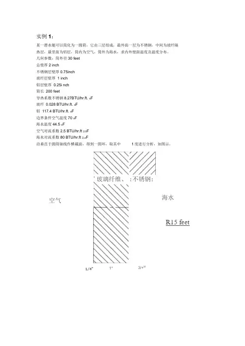
实例1:某一潜水艇可以简化为一圆筒,它由三层组成,最外面一层为不锈钢,中间为玻纤隔热层,最里面为铝层,筒内为空气,筒外为海水,求内外壁面温度及温度分布。
几何参数:筒外径30 feet总壁厚2 inch不锈钢层壁厚0.75inch玻纤层壁厚 1 inch铝层壁厚0.25i nch筒长200 feet导热系数不锈钢8.27BTU/hr.ft. o F玻纤0.028 BTU/hr.ft. o F铝117.4 BTU/hr.ft. o F边界条件空气温度70 o F海水温度44.5 o F空气对流系数2.5 BTU/hr.ft 2.0F海水对流系数80 BTU/hr.ft 2.o F沿垂直于圆筒轴线作横截面,得到一圆环,取其中1度进行分析,如图示。
空气'玻璃纤维、1*:不锈钢:3/+M海水R15 feet/filename ,Steady1 /title ,Steady-state thermal analysis of submarine /units ,BFT Ro=15 !外径(ft)Rss=15-(0.75/12) ! 不锈钢层内径ft) Rins=15-(1.75/12) ! 玻璃纤维层内径(ft) Ral=15-(2/12) ! 铝层内径(ft) Tair=70 ! 潜水艇内空气温度Tsea=44.5 !海水温度Kss=8.27 ! 不锈钢的导热系数(BTU/hr.ft.oF) Kins=0.028 ! 玻璃纤维的导热系数(BTU/hr.ft.oF)Kal=117.4 ! 铝的导热系数(BTU/hr.ft.oF) Hair=2.5 ! 空气的对流系数(BTU/hr.ft2.oF) Hsea=80 ! 海水的对流系数(BTU/hr.ft2.oF) prep7et,1,plane55 !定义二维热单元mp,kxx ,1,Kss !设定不锈钢的导热系数mp,kxx ,2,Kins !设定玻璃纤维的导热系数mp,kxx ,3,Kal !设定铝的导热系数pcirc,Ro,Rss,-0.5,0.5 !创建几何模型pcirc ,Rss,Rins ,-0.5 ,0.5 pcirc ,Rins,Ral,-0.5 ,0.5 aglue,all numcmp,area lesize,1,,,16 !设定划分网格密度lesize,4,,,4 lesize,14,,,5 lesize,16,,,2 Mshape,2 ! 设定为映射网格划分mat,1 amesh,1 mat,2 amesh,2 mat,3 amesh,3 /SOLUSFL,11,CONV ,HAIR ,,TAIR ! 施加空气对流边界SFL,1,CONV ,HSEA ,,TSEA !施加海水对流边界SOLVE /POST1PLNSOL !输出温度彩色云图finish实例2一圆筒形的罐有一接管,罐外径为 3英尺,壁厚为0.2英尺,接管外径为0.5英尺,壁厚为0.1英尺,罐与接管的轴线垂直且接管远离罐的端部。
第10 章热分析典型工程实例本章要点拉伸特征旋转特征扫掠特征混合特征孔特征壳特征本章案例某型号手机电池的散热分析冷库复合隔热板热量流动分析电子元器件散热装置温度分析10.1 工程实例1——某型号手机电池的散热分析该算例为某型手机电池的散热分析,如图10-1为某型号手机背面的照片,图中可见手机的电池的位置。
在手机工作时,电池可向外传递热量。
使用手机的读者应该都体会过手机电池发热的现象,特别是在长时间接打电话时,这种现象尤为明显。
本实例对某型号手机进行分析,电池的标准电压为3.7V,电池容量为750mAh。
试求手机开机状态下外壳的温度分布。
手机的各部分材料性能参数如表10.1所示。
图10-1 手机背面照片在计算分析过程中我们将手机看做三个组成部分:塑料外壳、手机内部材料和手机电池。
忽略手机内部线路和芯片,可以将手机电池看做唯一热源。
简化后的手机模型如图10-2所示,图中单位均为cm。
本实例拟采用Solid Tet 10node 87单元进行分析。
由于电池功率和环境温度均可视为恒定不变,因此分析类型为稳态。
图10-2 简化后的手机模型由电池的电压和电流可以算得电池的功率:==⨯=P UI 3.70.75 2.775W电池的体积为:3=⨯⨯=V0.040.010.050.00002m电池的发热量:3==Q P/V138750W/m——附带光盘“Ch10\实例10-1_start”——附带光盘“Ch10\实例10-1_end”——附带光盘“A VI\Ch10\10-1.avi”1、定义分析文件名1、选择Utility Menu>File>Change Jobname,在弹出的单元增添对话框中输入Example10-1,然后点击OK按钮。
2、选择Main Menu>Preferences,弹出Preferences for GUI Filtering对话框,点选Thermal复选框,单击OK按钮关闭该对话框。
ANSYS稳态热分析的基本过程和实例ANSYS稳态热分析的基本过程ANSYS热分析可分为三个步骤:前处理:建模、材料和⽹格分析求解:施加载荷计算后处理:查看结果1、建模①、确定jobname、title、unit;②、进⼊PREP7前处理,定义单元类型,设定单元选项;③、定义单元实常数;④、定义材料热性能参数,对于稳态传热,⼀般只需定义导热系数,它可以是恒定的,也可以随温度变化;⑤、创建⼏何模型并划分⽹格,请参阅《ANSYS Modeling and Meshing Guide》。
2、施加载荷计算①、定义分析类型●如果进⾏新的热分析:Command: ANTYPE, STATIC, NEWGUI: Main menu>Solution>-Analysis Type->New Analysis>Steady-state●如果继续上⼀次分析,⽐如增加边界条件等:Command: ANTYPE, STATIC, RESTGUI: Main menu>Solution>Analysis Type->Restart②、施加载荷可以直接在实体模型或单元模型上施加五种载荷(边界条件) :a、恒定的温度通常作为⾃由度约束施加于温度已知的边界上。
Command Family: DGUI:Main Menu>Solution>-Loads-Apply>-Thermal-Temperatureb、热流率热流率作为节点集中载荷,主要⽤于线单元模型中(通常线单元模型不能施加对流或热流密度载荷),如果输⼊的值为正,代表热流流⼊节点,即单元获取热量。
如果温度与热流率同时施加在⼀节点上则ANSYS读取温度值进⾏计算。
注意:如果在实体单元的某⼀节点上施加热流率,则此节点周围的单元要密⼀些,在两种导热系数差别很⼤的两个单元的公共节点上施加热流率时,尤其要注意。
此外,尽可能使⽤热⽣成或热流密度边界条件,这样结果会更精确些。
Workbench -Mechanical Introduction Introduction作业6.1稳态热分析作业6.1 –目标Workshop Supplement •本作业中,将分析下图所示泵壳的热传导特性。
•确切说是分析相同边界条件下的塑料(Polyethylene)泵壳和铝(Aluminum)泵壳。
)泵壳•目标是对比两种泵壳的热分析结果。
作业6.1 –假设Workshop Supplement 假设:•泵上的泵壳承受的温度为60度。
假设泵的装配面也处于60度下。
•泵的内表面承受90度的流体。
•泵的外表面环境用一个对流关系简化了的停滞空气模拟,温度为20度。
作业6.1 –Project SchematicWorkshop Supplement •打开Project 页•从Units菜单上确定:–项目单位设为Metric (kg, mm, s, C, mA, mV)–选择Display Values in Project Units…作业6.1 –Project SchematicWorkshop Supplement 1.在Toolbox中双击Steady-State Thermal创建一个新的Steady State Thermal(稳态Steady State Thermal热分析)系统。
1.2.在Geometry上点击鼠标右键选择p y,导入文Import Geometry件Pump_housing.x_t 2.…作业6.1 –Project SchematicWorkshop Supplement3.双击Engineering Data得到materialproperties(材料特性) 3.4.选中General Materials的同时,点击Aluminum Alloy和Polyethylene旁边的‘+’符号,把它们添加到项目中。
5.Return to Project(返回到项目)4.5.Workshop Supplement…作业6.1 –Project Schematic6.把Steady StateThermal 拖放到第一个系统的Geometry 上。
第四讲 热分析上机指导书CAD/CAM 实验室,USTC实验要求:1、通过对冷却栅管的热分析练习,熟悉用ANSYS 进展稳态热分析的根本过程,熟悉用直接耦合法、间接耦合法进展热应力分析的根本过程。
2、通过对铜块和铁块的水冷分析,熟悉用ANSYS 进展瞬态热分析的根本过程。
容1:冷却栅管问题问题描述:本实例确定一个冷却栅管〔图a 〕的温度场分布与位移和应力分布。
一个轴对称的冷却栅结构管为热流体,管外流体为空气。
冷却栅材料为不锈钢,特性如下:W/m ℃×109 MPa×10-5/℃边界条件:〔1〕管:压力:6.89 MPa流体温度:250 ℃对流系数249.23 W/m 2℃〔2〕管外:空气温度39℃对流系数:62.3 W/m 2℃假定冷却栅管无限长,根据冷却栅结构的对称性特点可以构造出的有限元模型如图b 。
其上下边界承受边界约束,管部承受均布压力。
练习1-1:冷却栅管的稳态热分析步骤:1. 定义工作文件名与工作标题1) 定义工作文件名:GUI: Utility Menu> File> Change Jobname ,在弹出的【ChangeJobname 】对话框中输入文件名Pipe_Thermal ,单击OK 按钮。
2) 定义工作标题:GUI: Utility Menu> File> Change Title ,在弹出的【Change Title 】对话框中2D Axisymmetrical Pipe Thermal Analysis ,单击OK 按钮。
3) 关闭坐标符号的显示:GUI: Utility Menu> PlotCtrls> Window Control> WindowOptions ,在弹出的【Window Options 】对话框的Location of triad 下拉列表框中选择No Shown 选项,单击OK 按钮。
本例题的主要部分为一个圆筒形罐,其上沿径向有一材料一样的接管(如图????所所示),罐内流动着450°F(232°C)的高温流体,接管内流动着100°F(38 °C)的低温流体,两个流体区域由薄壁管隔离。
罐的对流换热系数为250Btu/hr-ft2-o F(1420watts/m2-°K),接管的对流换热系数随管壁温度而变,它的热物理性能如表???所示。
要求计算罐与接管的温度分布。
表????6.5.1 预处理Step 1: 确定分析标题起动ANSYS后,开始一个分析,需要输入一个标题,按下面方法进行操作:1.选择Utility Menu> File> Change Title,弹出相应对话框2.输入Steady-state thermal analysis of pipe junction。
3.点击OK。
Step 2: 设置分析单位系统You need to specify units of measurement for the analysis. For this pipe junction example, measurements use the U. S. Customary system of units(based on inches). To specify this, type the command /UNITS,BIN in the ANSYS Input window and press ENTER.在分析之前,需要为分析系统设定单位系统,Step 3: Define the Element TypeThe example analysis uses a thermal solid element. To define it, do the following:1.Choose Main Menu> Preprocessor> Element Type> Add/Edit/Delete.The Element Types dialog box appears.2.Click on Add. The Library of Element Types dialog box appears.3.In the list on the left, scroll down and pick (highlight) "ThermalSolid." In the list on the right, pick "Brick20node 90."4.Click on OK.5.Click on Close to close the Element Types dialog box.Step 4: Define Material PropertiesTo define material properties for the analysis, perform these steps:1.Choose Main Menu> Preprocessor> Material Props> Material Models.The Define Material Model Behavior dialog box appears.2.In the Material Models Available window, double-click on thefollowing options: Thermal, Density. A dialog box appears.3.Enter .285 for DENS (Density), and click on OK. Material ModelNumber 1 appears in the Material Models Defined window on the left.4.In the Material Models Available window, double-click on thefollowing options: Conductivity, Isotropic. A dialog box appears.5.Click on the Add Temperature button four times. Four columns areadded.6.In the T1 through T5 fields, enter the following temperature values:70, 200, 300, 400, and 500. Select the row of temperatures bydragging the cursor across the text fields. Then copy thetemperatures by pressing Ctrl-c.7.In the KXX (Thermal Conductivity) fields, enter the followingvalues, in order, for each of the temperatures, then click on OK.Note that to keep the units consistent, each of the given values of KXX must be divided by 12. You can just input the fractions and have ANSYS perform the calculations.8.35/128.90/129.35/129.80/1210.23/128.In the Material Models Available window, double-click on SpecificHeat. A dialog box appears.9.Click on the Add Temperature button four times. Four columns areadded.10.With the cursor positioned in the T1 field, paste the fivetemperatures by pressing Ctrl-v.11.In the C (Specific Heat) fields, enter the following values, inorder, for each of the temperatures, then click on OK..113.117.119.122.12512.Choose menu path Material> New Model, then enter 2 for the newMaterial ID. Click on OK. Material Model Number 2 appears in the Material Models Defined window on the left.13.In the Material Models Available window, double-click on Convectionor Film Coef. A dialog box appears.14.Click on the Add Temperature button four times. Four columns areadded.15.With the cursor positioned in the T1 field, paste the fivetemperatures by pressing Ctrl-v.16.In the HF (Film Coefficient) fields, enter the following values,in order, for each of the temperatures. To keep the units consistent, each value of HF must be divided by 144. As in step 7, you can input the data as fractions and let ANSYS perform the calculations.426/144405/144352/144275/144221/14417.Click on the Graph button to view a graph of Film Coefficients vs.temperature, then click on OK.18.Choose menu path Material> Exit to remove the Define MaterialModel Behavior dialog box.19.Click on SAVE_DB on the ANSYS Toolbar.Step 5: Define Parameters for Modeling1.Choose Utility Menu> Parameters> Scalar Parameters. The ScalarParameters window appears.2.In the window's Selection field, enter the values shown below. (Donot enter the text in parentheses.) Press ENTER after typing in each value. If you make a mistake, simply retype the line containing the error.RI1=1.3 (Inside radius of the cylindrical tank)RO1=1.5 (Outside radius of the tank)Z1=2 (Length of the tank)RI2=.4 (Inside radius of the pipe)RO2=.5 (Outside radius of the pipe)Z2=2 (Length of the pipe)3.Click on Close to close the window.Step 6: Create the Tank and Pipe Geometry1.Choose Main Menu> Preprocessor> Modeling> Create> Volumes>Cylinder> By Dimensions. The Create Cylinder by Dimensions dialog box appears.2.Set the "Outer radius" field to RO1, the "Optional inner radius"field to RI1, the "Z coordinates" fieldsto 0 and Z1 respectively, and the "Ending angle" field to 90.3.Click on OK.4.Choose Utility Menu> WorkPlane> Offset WP by Increments. TheOffset WP dialog box appears.5.Set the "XY, YZ, ZX Angles" field to 0,-90.6.Click on OK.7.Choose Main Menu> Preprocessor> Modeling> Create> Volumes>Cylinder> By Dimensions. The Create Cylinder by Dimensions dialog box appears.8.Set the "Outer radius" field to RO2, the "Optional inner radius"field to RI2, the "Z coordinates" fieldsto 0 and Z2 respectively. Set the "Starting angle" fieldto -90 and the "Ending Angle" to 0.9.Click on OK.10.Choose Utility Menu> WorkPlane> Align WP with> GlobalCartesian.Step 7: Overlap the Cylinders1.Choose Main Menu> Preprocessor> Modeling> Operate> Booleans>Overlap> Volumes. The Overlap Volumes picking menu appears.2.Click on Pick All.Step 8: Review the Resulting ModelBefore you continue with the analysis, quickly review your model. To do so, follow these steps:1.Choose Utility Menu> PlotCtrls> Numbering. The Plot NumberingControls dialog box appears.2.Click the Volume numbers radio button to On, then click on OK.3.Choose Utility Menu> PlotCtrls> View Settings> ViewingDirection. A dialog box appears.4.Set the "Coords of view point" fields to (-3,-1,1), then click onOK.5.Review the resulting model.6.Click on SAVE_DB on the ANSYS Toolbar.Step 9: Trim Off Excess VolumesIn this step, delete the overlapping edges of the tank and the lower portion of the pipe.1.Choose Main Menu> Preprocessor> Modeling> Delete> Volume andBelow. The Delete Volume and Below picking menu appears.2.In the picking menu, type 3,4 and press the ENTER key. Then clickon OK in the Delete Volume and Below picking menu.Step 10: Create Component AREMOTEIn this step, you select the areas at the remote Y and Z edges of the tank and save them as a component called AREMOTE. To do so, perform these tasks:1.Choose Utility Menu> Select> Entities. The Select Entitiesdialog box appears.2.In the top drop down menu, select Areas. In the second drop downmenu, select By Location. Click on the Z Coordinates radio button.3.Set the "Min,Max" field to Z1.4.Click on Apply.5.Click on the Y Coordinates and Also Sele radio buttons.6.Set the "Min,Max" field to 0.7.Click on OK.8.Choose Utility Menu> Select> Comp/Assembly> Create Component.The Create Component dialog box appears.9.Set the "Component name" field to AREMOTE. In the "Component ismade of" menu, select Areas.10.Click on OK.Step 11: Overlay Lines on Top of AreasDo the following:1.Choose Utility Menu> PlotCtrls> Numbering. The Plot NumberingControls dialog box appears.2.Click the Area and Line number radio boxes to On and click on OK.3.Choose Utility Menu> Plot> Areas.4.Choose Utility Menu> PlotCtrls> Erase Options.5.Set "Erase between Plots" radio button to Off.6.Choose Utility Menu> Plot> Lines.7.Choose Utility Menu> PlotCtrls> Erase Options.8.Set "Erase between Plots" radio button to On.Step 12: Concatenate Areas and LinesIn this step, you concatenate areas and lines at the remote edges of the tank for mapped meshing. To do so, follow these steps:1.Choose Main Menu> Preprocessor> Meshing> Mesh> Volumes> Mapped>Concatenate> Areas. The Concatenate Areas picking menu appears.2.Click on Pick All.3.Choose Main Menu> Preprocessor> Meshing> Mesh> Volumes> Mapped>Concatenate> Lines. A picking menu appears.4.Pick (click on) lines 12 and 7 (or enter in the picker).5.Click on Apply.6.Pick lines 10 and 5 (or enter in picker).7.Click on OK.Step 13: Set Meshing Density Along Lines1.Choose Main Menu> Preprocessor> Meshing> Size Cntrls>ManualSize>Lines> Picked Lines. The Element Size on Picked Lines picking menu appears.2.Pick lines 6 and 20 (or enter in the picker) .3.Click on OK. The Element Sizes on Picked Lines dialog box appears.4.Set the "No. of element divisions" field to 4.5.Click on OK.6.Choose Main Menu> Preprocessor> Meshing> Size Cntrls>ManualSize> Lines> Picked Lines. A picking menu appears.7.Pick line 40 (or enter in the picker).8.Click on OK. The Element Sizes on Picked Lines dialog box appears.9.Set the "No. of element divisions" field to 6.10.Click on OK.Step 14: Mesh the ModelIn this sequence of steps, you set the global element size, set mapped meshing, then mesh the volumes.1.Choose Utility Menu> Select> Everything.2.Choose Main Menu> Preprocessor> Meshing> Size Cntrls>ManualSize> Global> Size. The Global Element Sizes dialog boxappears.3.Set the "Element edge length" field to 0.4 and click on OK.4.Choose Main Menu> Preprocessor> Meshing> Mesher Opts. TheMesher Options dialog box appears.5.Set the Mesher Type radio button to Mapped and click on OK. The SetElement Shape dialog box appears.6.In the 2-D shape key drop down menu, select Quad and click on OK.7.Click on the SAVE_DB button on the Toolbar.8.Choose Main Menu> Preprocessor> Meshing> Mesh> Volumes> Mapped>4 to 6 sided. The Mesh Volumes picking menu appears. Click on PickAll. In the Graphics window, ANSYS builds the meshed model. If a shape testing warning message appears, review it and click Close.Step 15: Turn Off Numbering and Display Elements1.Choose Utility Menu> PlotCtrls> Numbering. The Plot NumberingControls dialog box appears.2.Set the Line, Area, and Volume numbering radio buttons to Off.3.Click on OK.Step 16: Define the Solution Type and OptionsIn this step, you tell ANSYS that you want a steady-state solution that uses a program-chosen Newton-Raphson option.1.Choose Main Menu> Solution> Analysis Type> New Analysis. The NewAnalysis dialog box appears.2.Click on OK to choose the default analysis type (Steady-state).3.Choose Main Menu> Solution> Analysis Type> Analysis Options.The Static or Steady-State dialog box appears.4.Click on OK to accept the default (“Program-chosen”) for"Newton-Raphson option."Step 17: Set Uniform Starting TemperatureIn a thermal analysis, set a starting temperature.1.Choose Main Menu> Solution> Define Loads> Apply> Thermal>Temperature> Uniform Temp. A dialog box appears.2.Enter 450 for "Uniform temperature." Click on OK.Step 18: Apply Convection LoadsThis step applies convection loads to the nodes on the inner surface of the tank.1.Choose Utility Menu> WorkPlane> Change Active CS to> GlobalCylindrical.2.Choose Utility Menu> Select> Entities. The Select Entitiesdialog box appears.3.Select Nodes and By Location, and click on the X Coordinates andFrom Full radio buttons.4.Set the "Min,Max" field to RI1 and click on OK.5.Choose Main Menu> Solution> Define Loads> Apply> Thermal>Convection> On Nodes. The Apply CONV on Nodes picking menu appears.6.Click on Pick All. The Apply CONV on Nodes dialog box appears.7.Set the "Film coefficient" field to 250/144.8.Set the "Bulk temperature" field to 450.9.Click on OK.Step 19: Apply Temperature Constraints to AREMOTE Component1.Choose Utility Menu> Select> Comp/Assembly> SelectComp/Assembly. A dialog box appears.2.Click on OK to select component AREMOTE.3.Choose Utility Menu> Select> Entities. The Select Entitiesdialog box appears.4.Select Nodes and Attached To, and click on the Areas,All radiobutton. Click on OK.5.Choose Main Menu> Solution> Define Loads> Apply> Thermal>Temperature> On Nodes. The Apply TEMP on Nodes picking menu appears.6.Click on Pick All. A dialog box appears.7.Set the "Load TEMP value" field to 450.8.Click on OK.9.Click on SAVE_DB on the ANSYS Toolbar.Step 20: Apply Temperature-Dependent ConvectionIn this step, apply a temperature-dependent convection load on the inner surface of the pipe.1.Choose Utility Menu> WorkPlane> Offset WP by Increments. Adialog box appears.2.Set the "XY,YZ,ZX Angles" field to 0,-90, then click on OK.3.Choose Utility Menu> WorkPlane> Local Coordinate Systems>Create Local CS> At WP Origin. The Create Local CS at WP Origin dialog box appears.4.On the "Type of coordinate system" menu, select "Cylindrical 1" andclick on OK.5.Choose Utility Menu> Select> Entities. The Select Entitiesdialog box appears.6.Select Nodes, and By Location, and click on the X Coordinates radiobutton.7.Set the "Min,Max" field to RI2.8.Click on OK.9.Choose Main Menu> Solution> Define Loads> Apply> Thermal>Convection> On Nodes. The Apply CONV on Nodes picking menu appears.10.Click on Pick All. A dialog box appears.11.Set the "Film coefficient" field to -2.12.Set the "Bulk temperature" field to 100.13.Click on OK.14.Choose Utility Menu> Select> Everything.15.Choose Utility Menu> PlotCtrls> Symbols. The Symbols dialog boxappears.16.On the "Show pres and convect as" menu, select Arrows, then clickon OK.17.Choose Utility Menu> Plot> Nodes. The display in the GraphicsWindow changes to show you a plot of nodes.Step 21: Reset the Working Plane and Coordinates1.To reset the working plane and default Cartesian coordinate system,choose Utility Menu> WorkPlane> Change Active CS to> GlobalCartesian.2.Choose Utility Menu> WorkPlane> Align WP With> Global Cartesian.Step 22: Set Load Step OptionsFor this example analysis, you need to specify 50 substeps with automatic time stepping.1.Choose Main Menu> Solution> Load Step Options> Time/Frequenc>Time and Substps. The Time and Substep Options dialog box appears.2.Set the "Number of substeps" field to 50.3.Set "Automatic time stepping" radio button to On.4.Click on OK.Step 23: Solve the Model1.Choose Main Menu> Solution> Solve> Current LS. The ANSYS programdisplays a summary of the solution options in a /STAT commandwindow.2.Review the summary.3.Choose Close to close the /STAT command window.4.Click on OK in the Solve Current Load Step dialog box.5.Click Yes in the Verify message window.6.The solution runs. When the Solution is done! window appears, clickon Close.Step 24: Review the Nodal Temperature Results1.Choose Utility Menu> PlotCtrls> Style> Edge Options. The EdgeOptions dialog box appears.2.Set the "Element outlines" field to "Edge only" for contour plotsand click on OK.3.Choose Main Menu> General Postproc> Plot Results> Contour Plot>Nodal Solu. The Contour Nodal Solution Data dialog box appears.4.For "Item to be contoured," pick "DOF solution" from the list onthe left, then pick "Temperature TEMP" from the list on the right.5.Click on OK. The Graphics window displays a contour plot of thetemperature results.Step 25: Plot Thermal Flux VectorsIn this step, you plot the thermal flux vectors at the intersection of the pipe and tank.1.Choose Utility Menu> WorkPlane> Change Active CS to> SpecifiedCoord Sys. A dialog box appears.2.Set the "Coordinate system number" field to 11.3.Click on OK.4.Choose Utility Menu> Select> Entities. The Select Entitiesdialog box appears.5.Select Nodes and By Location, and click the X Coordinates radiobutton.6.Set the "Min,Max" field to RO2.7.Click on Apply.8.Select Elements and Attached To, and click the Nodes radio button.9.Click on Apply.10.Select Nodes and Attached To, then click on OK.11.Choose Main Menu> General Postproc> Plot Results> Vector Plot>Predefined. A dialog box appears.实用标准文案12.For "Vector item to be plotted," choose "Flux & gradient" from thelist on the left and choose "Thermal flux TF" from the list on the right.13.Click on OK. The Graphics Window displays a plot of thermal fluxvectors.Step 26: Exit from ANSYSTo leave the ANSYS program, click on the QUIT button in the Toolbar. Choose an exit option and click on OK.文档大全。