Computing the effective diffusivity using a spectral method

如何平衡科技与生活英语作文In today's fast-paced world, the rapid development of technology has undoubtedly brought numerous benefits to our lives. However, many individuals find themselves struggling to maintain a healthy balance between their reliance on technology and their personal well-being. This essay aims to explore effective ways to strike a balance between technology and life without using common transitional phrases such as "firstly," "secondly," "however," "but," "among them," "furthermore," "in conclusion," or similar words.Living in the digital age, it is essential for us to acknowledge the potential negative impacts of excessive screen time and constant connectivity. Firstly, we must develop a conscious awareness of how much time we spend on our electronic devices. Engaging in activities such as setting specific time limits for using social media apps or turning off notifications during certain hours can help create a healthier relationship with our technology.In addition to managing our screen time, it is importantfor us to prioritize real-life connections and interactions. Instead of solely relying on virtual communication, we should make an effort to engage in face-to-face conversations and spend quality time with family and friends. By doing so, we can cultivate meaningful relationships that go beyond mere superficial connections.Furthermore, finding alternative ways to relax and unwind from the demands of technology is crucial for achieving balance in our lives. Rather than scrolling through endless newsfeeds or binge-watching television shows every evening, consider exploring hobbies that allow you to disconnectfrom your devices completely. Whether it's reading books, engaging in physical activities like hiking or painting, or simply spending time in nature, these activities provide an opportunity for self-reflection and rejuvenation.Moreover, practicing mindfulness can significantly help us achieve a healthier balance between technology and life. Mindfulness involves being fully present in the moment without judgment or attachment. Through regular meditationor other mindfulness techniques, we can increase our awareness of how we interact with technology while learning to detach ourselves from its constant grip. This allows us to appreciate the present moment and find a sense of peace amidst the noise and distractions of the digital world.Lastly, it is crucial to establish boundaries between our personal and professional lives. In today's interconnected world, many individuals find themselves constantly accessible due to the advancements in communication technology. However, this constant availability can lead to burnout and blur the line between work and personal life. Setting clear limits on when we are available for work-related matters can help create a healthy separation between the two realms.To summarize, maintaining a balance between technology and life requires conscious efforts in managing screen time, prioritizing real-life connections, exploring alternative ways to relax, practicing mindfulness techniques, and establishing boundaries between personal and professional lives. By integrating these strategies into our dailyroutines, we can navigate the digital landscape more effectively while ensuring our well-being remains a priority.。

In the realm of future technology,there are myriad possibilities that can revolutionize the way we live,work,and interact with the world around us.Here are some key areas where advancements are expected to make a significant impact:1.Artificial Intelligence AI:AI is poised to become an integral part of our daily lives, from personal assistants that can anticipate our needs to advanced machine learning algorithms that can solve complex problems in fields such as medicine,finance,and environmental science.2.Quantum Computing:The development of quantum computers will enable us to process information at unprecedented speeds,opening up new frontiers in cryptography, material science,and complex system modeling.3.Renewable Energy Technologies:As the world moves towards sustainability, advancements in solar,wind,and other renewable energy sources will become more efficient and costeffective,reducing our reliance on fossil fuels and mitigating the effects of climate change.4.Biotechnology and Genetic Engineering:The ability to edit genes will not only revolutionize medicine by allowing for the treatment and prevention of genetic disorders but also has implications for agriculture,where crops can be engineered to be more resistant to pests and environmental stress.5.Space Exploration and Colonization:With the potential for manned missions to Mars and the establishment of lunar bases,space technology will advance our understanding of the universe and possibly provide solutions to some of Earths most pressing issues,such as resource scarcity.6.Autonomous Vehicles:Selfdriving cars,drones,and other autonomous transportation systems will transform the way we commute,reducing traffic congestion,and improving safety on the roads.7.Virtual Reality VR and Augmented Reality AR:These technologies will become more immersive and integrated into our daily lives,offering new ways to learn,work,and experience entertainment.8.Advanced Robotics:Robots will become more sophisticated,capable of performing complex tasks in manufacturing,healthcare,and even in our homes,assisting with daily chores and providing companionship.9.Nanotechnology:The manipulation of matter on an atomic and molecular scale will lead to breakthroughs in materials science,medicine,and electronics,potentially leading to stronger,lighter,and more efficient products.10.5G and Beyond:The next generation of wireless technology will enable faster,more reliable internet connections,facilitating the Internet of Things IoT and smart cities, where devices and infrastructure communicate seamlessly to improve efficiency and quality of life.11.Blockchain Technology:Beyond cryptocurrencies,blockchains secure,decentralized nature will be applied to various sectors,including supply chain management,voting systems,and healthcare records management.12.Advanced Materials:The development of new materials with unique properties,such as superconductors,graphene,and metamaterials,will drive innovation in electronics, energy storage,and construction.As we venture further into the future,the convergence of these technologies will likely lead to innovations that we cannot yet imagine,continually reshaping our world in ways that are as exciting as they are challenging.The key to harnessing the potential of future technology lies in ethical considerations,education,and a proactive approach to integrating these advancements into society for the betterment of all.。

比较人工智能在中国和美国的发展的英语作文Title: Comparing the Development of Artificial Intelligence in China and the United StatesIn the realm of technological advancement, Artificial Intelligence (AI) stands as a beacon of innovation, propelling societies forward into a future filled with boundless possibilities. Both China and the United States, as global leaders in this field, have invested heavily in AI research and development, each forging its unique path towards technological supremacy. A comparison of their AI landscapes reveals intriguing similarities and striking differences that reflect their respective economic, political, and cultural contexts.Investment and FundingBoth countries have poured significant resources into AI research, but their approaches differ. The United States boasts a long history of innovation and research funding from both the government and private sectors. Silicon Valley, in particular, has emerged as a hub for AI startups, attracting venture capitalists and tech giants alike. China, on the other hand, has embarked on a national strategy to become a global AI powerhouse, with substantial investments from the government, state-owned enterprises, and a rapidly growing private sector. This top-down approach has accelerated China's progress in AI, especially in areas such as facial recognition, autonomous vehicles, and smart cities.Research FocusWhile both countries prioritize AI research across various domains, their areas of focus exhibit distinct patterns. The United States tends to emphasize fundamental research andtheory-driven innovations, nurturing an environment conducive to breakthrough discoveries. This approach has led to advancements in areas like natural language processing, machine learning algorithms, and quantum computing. China, meanwhile, has placed a strong emphasis on practical applications and industrialization of AI technologies. This has resulted in rapid deployments of AI in sectors like manufacturing, healthcare, and public services, transforming industries and improving efficiency.Regulation and EthicsThe regulatory landscapes surrounding AI in China and the US also differ significantly. The United States has a more decentralized approach to AI regulation, with various state and federal agencies tackling specific aspects of the technology. This has led to a more nuanced and often contentious debate on issues like data privacy, algorithmic bias, and ethical AI. China, on the other hand, has taken a more centralized approach, issuing national-level guidelines and regulations to guide the development and deployment of AI. However, concerns about data privacy and the potential misuse of AI technologies by the government have persisted. Collaboration and CompetitionBoth countries recognize the importance of international collaboration in AI research and development, yet they also compete fiercely for global dominance. The United States maintains strong partnerships with other Western nations and multinational corporations, fostering a global network of AI innovators. China, too, has sought collaborations with countries around the world, particularly in the Belt and Road Initiative, promoting AItechnologies and standards abroad. However, the competition between the two nations in the AI sphere is intense, with each striving to maintain its technological edge.In conclusion, the development of Artificial Intelligence in China and the United States is a complex interplay of investment, research focus, regulation, and international relations. While both countries share a commitment to advancing AI technologies, their distinct approaches reflect their unique economic, political, and cultural contexts. As the race for AI supremacy continues, it remains to be seen how these two global leaders will shape the future of this transformative technology.。

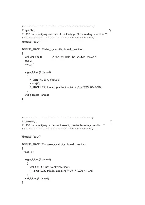
/***********************************************************************//* vprofile.c */ /* UDF for specifying steady-state velocity profile boundary condition *//***********************************************************************/#include "udf.h"DEFINE_PROFILE(inlet_x_velocity, thread, position){real x[ND_ND]; /* this will hold the position vector */real y;face_t f;begin_f_loop(f, thread){F_CENTROID(x,f,thread);y = x[1];F_PROFILE(f, thread, position) = 20. - y*y/(.0745*.0745)*20.;}end_f_loop(f, thread)}/**********************************************************************//* unsteady.c */ /* UDF for specifying a transient velocity profile boundary condition *//**********************************************************************/#include "udf.h"DEFINE_PROFILE(unsteady_velocity, thread, position){face_t f;begin_f_loop(f, thread){real t = RP_Get_Real("flow-time");F_PROFILE(f, thread, position) = 20. + 5.0*sin(10.*t);}end_f_loop(f, thread)}/******************************************************************//* UDF that adds momentum source term and derivative to duct flow */ /******************************************************************/#include "udf.h"#define CON 20.0DEFINE_SOURCE(cell_x_source, cell, thread, dS, eqn){real source;if (C_T(cell,thread) <= 288.){/* source term */source = -CON*C_U(cell,thread);/* derivative of source term w.r.t. x-velocity. */dS[eqn] = -CON;}elsesource = dS[eqn] = 0.;return source;}/*********************************************************************//* UDF for specifying a temperature-dependent viscosity property */ /*********************************************************************/#include "udf.h"DEFINE_PROPERTY(cell_viscosity, cell, thread){real mu_lam;real temp = C_T(cell, thread);if (temp > 288.)mu_lam = 5.5e-3;else if (temp > 286.)mu_lam = 143.2135 - 0.49725 * temp;elsemu_lam = 1.;return mu_lam;}/**************************************************************//* rate.c *//* UDF for specifying a reaction rate in a porous medium *//**************************************************************/#include "udf.h"#define K1 2.0e-2#define K2 5.DEFINE_VR_RATE(user_rate, c, t, r, mole_weight, species_mf, rate, rr_t) {real s1 = species_mf[0];real mw1 = mole_weight[0];if (FLUID_THREAD_P(t) && THREAD_VAR(t).fluid.porous)*rate = K1*s1/pow((1.+K2*s1),2.0)/mw1;else*rate = 0.;}/***********************************************************************//* UDF for computing the magnitude of the gradient of T^4 */ /***********************************************************************/#include "udf.h"/* Define which user-defined scalars to use. */enum{T4,MAG_GRAD_T4,N_REQUIRED_UDS};DEFINE_ADJUST(adjust_fcn, domain){Thread *t;cell_t c;face_t f;/* Make sure there are enough user-defined scalars. */if (n_uds < N_REQUIRED_UDS)Internal_Error("not enough user-defined scalars allocated");/* Fill first UDS with temperature raised to fourth power. */ thread_loop_c (t,domain){if (NULL != THREAD_STORAGE(t,SV_UDS_I(T4))){begin_c_loop (c,t){real T = C_T(c,t);C_UDSI(c,t,T4) = pow(T,4.);}end_c_loop (c,t)}}thread_loop_f (t,domain){if (NULL != THREAD_STORAGE(t,SV_UDS_I(T4))){begin_f_loop (f,t){real T = 0.;if (NULL != THREAD_STORAGE(t,SV_T))T = F_T(f,t);else if (NULL != THREAD_STORAGE(t->t0,SV_T))T = C_T(F_C0(f,t),t->t0);F_UDSI(f,t,T4) = pow(T,4.);}end_f_loop (f,t)}}/* Fill second UDS with magnitude of gradient. */thread_loop_c (t,domain){if (NULL != THREAD_STORAGE(t,SV_UDS_I(T4)) &&NULL != T_STORAGE_R_NV(t,SV_UDSI_G(T4))){begin_c_loop (c,t){C_UDSI(c,t,MAG_GRAD_T4) = NV_MAG(C_UDSI_G(c,t,T4));}end_c_loop (c,t)}}thread_loop_f (t,domain){if (NULL != THREAD_STORAGE(t,SV_UDS_I(T4)) &&NULL != T_STORAGE_R_NV(t->t0,SV_UDSI_G(T4))){begin_f_loop (f,t){F_UDSI(f,t,MAG_GRAD_T4)=C_UDSI(F_C0(f,t),t->t0,MAG_GRAD_T4);}end_f_loop (f,t)}}}/**************************************************************//* Implementation of the P1 model using user-defined scalars *//**************************************************************/#include "udf.h"/* Define which user-defined scalars to use. */enum{P1,N_REQUIRED_UDS};static real abs_coeff = 1.0; /* absorption coefficient */static real scat_coeff = 0.0; /* scattering coefficient */static real las_coeff = 0.0; /* linear-anisotropic *//* scattering coefficient */static real epsilon_w = 1.0; /* wall emissivity */DEFINE_ADJUST(p1_adjust, domain){/* Make sure there are enough user defined-scalars. */if (n_uds < N_REQUIRED_UDS)Internal_Error("not enough user-defined scalars allocated");}DEFINE_SOURCE(energy_source, c, t, dS, eqn){dS[eqn] = -16.*abs_coeff*SIGMA_SBC*pow(C_T(c,t),3.);return -abs_coeff*(4.*SIGMA_SBC*pow(C_T(c,t),4.) - C_UDSI(c,t,P1)); }DEFINE_SOURCE(p1_source, c, t, dS, eqn){dS[eqn] = -abs_coeff;return abs_coeff*(4.*SIGMA_SBC*pow(C_T(c,t),4.) - C_UDSI(c,t,P1)); }DEFINE_DIFFUSIVITY(p1_diffusivity, c, t, i){return 1./(3.*abs_coeff + (3. - las_coeff)*scat_coeff);}DEFINE_PROFILE(p1_bc, thread, position){face_t f;real A[ND_ND],At;real dG[ND_ND],dr0[ND_ND],es[ND_ND],ds,A_by_es;real aterm,alpha0,beta0,gamma0,Gsource,Ibw;real Ew = epsilon_w/(2.*(2. - epsilon_w));Thread *t0=thread->t0;/* Do nothing if areas aren't computed yet or not next to fluid. */if (!Data_Valid_P() || !FLUID_THREAD_P(t0)) return;begin_f_loop (f,thread){cell_t c0 = F_C0(f,thread);BOUNDARY_FACE_GEOMETRY(f,thread,A,ds,es,A_by_es,dr0);At = NV_MAG(A);if (NULLP(T_STORAGE_R_NV(t0,SV_UDSI_G(P1))))Gsource = 0.; /* if gradient not stored yet */elseBOUNDARY_SECONDARY_GRADIENT_SOURCE(Gsource,SV_UDSI_G(P1),dG,es,A_by_es,1.);gamma0 = C_UDSI_DIFF(c0,t0,P1);alpha0 = A_by_es/ds;beta0 = Gsource/alpha0;aterm = alpha0*gamma0/At;Ibw = SIGMA_SBC*pow(WALL_TEMP_OUTER(f,thread),4.)/M_PI;/* Specify the radiative heat flux. */F_PROFILE(f,thread,position) =aterm*Ew/(Ew + aterm)*(4.*M_PI*Ibw - C_UDSI(c0,t0,P1) + beta0);}end_f_loop (f,thread)}DEFINE_HEAT_FLUX(heat_flux, f, t, c0, t0, cid, cir){real Ew = epsilon_w/(2.*(2. - epsilon_w));cid[0] = Ew * F_UDSI(f,t,P1);cid[3] = 4.0 * Ew * SIGMA_SBC;}#define DEFINE_ADJUST(name, domain) \void name(Domain *domain)#define DEFINE_INIT(name, domain) \void name(Domain *domain)#define DEFINE_ON_DEMAND(name) \void name(void)#define DEFINE_RW_FILE(name, fp) \void name(FILE *fp)#define DEFINE_CG_MOTION(name, dt, vel, omega, time, dtime) \void name(void *dt, real vel[], real omega[], real time, real dtime)#define DEFINE_DIFFUSIVITY(name, c, t, i)real name(cell_t c, Thread *t, int i)#define DEFINE_GEOM(name, d, dt, position) \void name(Domain *d, void *dt, real *position)#define DEFINE_GRID_MOTION(name, d, dt, time, dtime) \void name(Domain *d, void *dt, real time, real dtime)#define DEFINE_HEAT_FLUX(name, f, t, c0, t0, cid, cir) \void name(face_t f, Thread *t, cell_t c0, \Thread *t0, real cid[], real cir[])#define DEFINE_NOX_RATE(name, c, t, NOx) \void name(cell_t c, Thread *t, NOx_Parameter *NOx)#define DEFINE_PROFILE(name, t, i) \void name(Thread *t, int i)#define DEFINE_PROPERTY(name, c, t) \real name(cell_t c, Thread *t)#define DEFINE_SCAT_PHASE_FUNC(name, c, f) \real name(real c, real *f)#define DEFINE_SOURCE(name, c, t, dS, i) \real name(cell_t c, Thread *t, real dS[], int i)#define DEFINE_SR_RATE(name, f, t, r, mw, yi, rr) \void name(face_t c, Thread *t, \Reaction *r, real *mw, real *yi, real *rr)#define DEFINE_TURB_PREMIX_SOURCE(name, c, t, turbulent_flame_speed, sourc e) \void name(cell_t c, Thread *t, real *turbulent_flame_speed, real *source)#define DEFINE_TURBULENT_VISCOSITY(name, c, t) real name(cell_t c, Thread * t)#define DEFINE_UDS_FLUX(name, f, t, i) \real name(face_t f, Thread *t, int i)#define DEFINE_UDS_UNSTEADY(name, c, t, i, apu, su) \void name(cell_t c, Thread *t, int i, real *apu, real *su)#define DEFINE_VR_RATE(name, c, t, r, mw, yi, rr, rr_t) \void name(cell_t c, Thread *t, \Reaction *r, real *mw, real *yi, \real *rr, real *rr_t)#define DEFINE_CAVITATION_RATE(name, c, t, p, rhoV, rhoL, vofV, p_v, n_b, m_d ot) \void name(cell_t c, Thread *t, real *p, real *rhoV, real *rhoL, real *vofV, \ real *p_v, real *n_b, real *m_dot)#define DEFINE_DRIFT_DIAM(name, c, t) \real name(cell_t c, Thread *t)#define DEFINE_EXCHANGE_PROPERTY(name, c, mixture_thread, \second_column_phase_index, first_column_phase_index) \real name(cell_t c, Thread *mixture_thread, int second_column_phase_index,\ int first_column_phase_index)#define DEFINE_VECTOR_EXCHANGE_PROPERTY(name, c, mixture_thread, \ second_column_phase_index, first_column_phase_index, vector_result) \void name(cell_t c, Thread *mixture_thread, int second_column_phase_index,\int first_column_phase_index, real *vector_result)#define DEFINE_DPM_BODY_FORCE(name, p, i) \real name(Tracked_Particle *p, int i)#define DEFINE_DPM_DRAG(name, Re) \real name(real Re)#define DEFINE_DPM_SOURCE(name, c, t, S, strength, p) \void name(cell_t c, Thread *t, dpms_t *S, \real strength, Tracked_Particle *p)#define DEFINE_DPM_PROPERTY(name, c, t, p) \real name(cell_t c, Thread *t, Tracked_Particle *p)#define DEFINE_DPM_OUTPUT(name, header, fp, p, t, plane) \void name(int header, FILE *fp, \Tracked_Particle *p, Thread *t, Plane *plane)#define DEFINE_DPM_EROSION(name, p, t, f, normal, alpha, Vmag, mdot) \void name(Tracked_Particle *p, Thread *t, \face_t f, real normal[], real alpha, \real Vmag, real mdot)#define DEFINE_DPM_SCALAR_UPDATE(name, c, t, initialize, p) \void name(cell_t c, Thread *t, int initialize, \Tracked_Particle *p)#define DEFINE_DPM_LAW(name, p, ci)void name(Tracked_Particle *p, int ci)#define DEFINE_DPM_SWITCH(name, p, ci) \void name(Tracked_Particle *p, int ci)#define DEFINE_DPM_INJECTION_INIT(name, I) \void name(Injection *I)。

现代科学对创新的促进作用英语作文In today's era of rapid technological advancement, the role of modern science in driving innovation cannot be overstated. The intersection of science and innovation has led to unprecedented breakthroughs in various fields, ranging from medicine to engineering, technology to environmental science. This essay explores the profound impact of modern science on innovation and how it has reshaped our world.Firstly, modern science has provided a robust foundation for innovation by constantly pushing the boundaries of knowledge. The advancement of scientific theories and discoveries has led to the development of new technologies and methods. For instance, the understanding of quantum physics has led to the creation of transistors and computers, which have revolutionized the way we live and work. Similarly, the principles of evolutionary biology have informed genetic engineering and biotechnology, enabling us to develop new crops and treatments for diseases.Secondly, modern science has fostered a culture of curiosity and exploration, which is essential for innovation. Scientific research鼓励s us to question established beliefs and explore uncharted territories. This curiosity-driven approach has led to numerous breakthroughs in areas such as space exploration, where scientific inquiries have pushed the boundaries of human understanding and led to remarkable technological advancements.Moreover, modern science has enabled globalcollaboration and knowledge sharing, which has accelerated the pace of innovation. The internet and other digital technologies have made it possible for scientists and researchers to collaborate on projects regardless of their geographical location. This has led to the emergence of global research networks and consortiums, which have been instrumental in making significant scientific breakthroughs. Additionally, modern science has provided us with powerful tools and technologies that enable us to test and validate new ideas more efficiently. For instance, computational modeling and simulation have allowedscientists to test their hypotheses without having toconduct expensive and time-consuming experiments. Thesetools have significantly reduced the time and cost of research, enabling more rapid iteration and refinement of ideas.In conclusion, modern science has played a pivotal role in promoting innovation in various fields. Its impact isfelt across all sectors of society, from medicine and technology to environmental science and beyond. As we continue to make scientific discoveries and develop new technologies, the potential for further innovation is limitless. It is through the continued advancement of science that we will be able to address the challenges of our time and create a better future for all.**现代科学：创新的催化剂**在当今科技飞速发展的时代，现代科学对创新的推动作用不容忽视。

对计算机发展的设想英文回答：The rapid advancement of computer technology has revolutionized various aspects of human life, transforming the way we communicate, learn, work, and entertain ourselves. As we look towards the future, it is exciting to speculate on the potential developments and innovationsthat could shape the next generation of computing.One significant area of exploration lies in the convergence of artificial intelligence (AI) and quantum computing. AI-powered systems are already demonstrating remarkable capabilities in areas such as natural language processing, image recognition, and decision-making. When combined with the immense computational power of quantum computers, AI systems could potentially solve complex problems that are currently intractable for classical computers. This could lead to breakthroughs in fields such as drug discovery, materials science, and financialmodeling.Another promising area is the development of neuromorphic computing, which aims to mimic the structure and functionality of the human brain. Neuromorphic chipsare designed to process and store information in a manner similar to biological neurons, enabling them to perform complex tasks such as pattern recognition, learning, and adaptation. By harnessing the power of neuromorphic computing, we could create computers that are moreefficient, intelligent, and capable of handling tasks that are currently beyond the reach of traditional computing systems.Furthermore, the concept of edge computing is gaining traction. Edge computing involves distributingcomputational resources and data storage closer to the devices and users that need them. This approach reduces latency and improves performance for real-time applications, such as autonomous vehicles, smart cities, and industrial automation. By bringing computing closer to the edge, wecan enable faster response times, reduce bandwidthrequirements, and improve overall system efficiency.Additionally, the rise of virtual and augmented reality (VR/AR) is transforming the way we interact with thedigital world. VR/AR headsets allow us to experience immersive virtual environments and overlay digital information onto the real world. As VR/AR technology continues to advance, we can expect to see even more innovative applications in fields such as gaming, education, healthcare, and remote collaboration.In terms of hardware, the development of new materials and fabrication techniques is pushing the boundaries of computing performance. Carbon nanotubes, graphene, andother advanced materials are enabling the creation of smaller, faster, and more energy-efficient devices. Additionally, the emergence of 3D printing and additive manufacturing is revolutionizing the way we design and produce computer components, allowing for greater customization and flexibility.Finally, it is important to consider the ethical andsocietal implications of rapid technological advancements. As computers become more powerful and autonomous, we needto address issues such as data privacy, job displacement, and the potential misuse of technology. By engaging in responsible innovation and fostering collaboration between technologists, policymakers, and ethicists, we can harness the transformative power of computing while mitigating potential risks.中文回答：随着计算机技术的飞速发展，各个方面的彻底改变人们的生活，改变了人们交流、学习、工作和娱乐方式。

Algorithmic Efficiency inComputational Problemsrefers to the ability of an algorithm to solve a problem in the most efficient manner possible. In computer science, algorithmic efficiency is a key concept that plays a crucial role in the design and analysis of algorithms. It is important to analyze and compare the efficiency of different algorithms in order to determine the best algorithm for a given problem.There are several factors that contribute to the efficiency of an algorithm, including time complexity, space complexity, and the quality of the algorithm design. Time complexity refers to the amount of time it takes for an algorithm to solve a problem, while space complexity refers to the amount of memory space required by an algorithm to solve a problem. The quality of algorithm design includes factors such as the choice of data structures and the way the algorithm is implemented.One important measure of algorithmic efficiency is the big O notation, which provides an upper bound on the growth rate of an algorithm. The big O notation allows us to compare the efficiency of different algorithms and make informed decisions about which algorithm to use for a particular problem. For example, an algorithm with a time complexity of O(n) is considered more efficient than an algorithm with a time complexity of O(n^2) for large input sizes.In order to improve the efficiency of algorithms, it is important to understand the theory behind algorithm design and analysis. This includes understanding different algorithm design techniques such as divide and conquer, dynamic programming, and greedy algorithms. By using these techniques, it is possible to design algorithms that are more efficient and can solve problems in a faster and more resource-efficient manner.In addition to understanding algorithm design techniques, it is also important to consider the specific characteristics of the problem at hand when designing algorithms. For example, some problems may have specific constraints that can be exploited toimprove algorithm efficiency. By taking into account these constraints, it is possible to design algorithms that are tailored to a specific problem and can solve it more efficiently.Another key aspect of algorithmic efficiency is the implementation of algorithms. The choice of programming language, data structures, and optimization techniques can all impact the efficiency of an algorithm. By optimizing the implementation of an algorithm, it is possible to reduce its time and space complexity and improve its overall efficiency.Overall, algorithmic efficiency is a fundamental concept in computer science that plays a crucial role in the design and analysis of algorithms. By understanding the theory behind algorithm design and analysis, and by carefully considering the specific characteristics of the problem at hand, it is possible to design algorithms that are efficient, fast, and resource-efficient. This can lead to significant improvements in the performance of computational problems and the development of more effective software applications.。

介绍量子计算与生活的关系英语作文全文共3篇示例，供读者参考篇1Quantum computing, as a revolutionary technology, has attracted increasing attention in recent years. It has been praised for its potential to solve complex problems at a speed unimaginable by traditional computers. But how does quantum computing relate to our daily lives? Let's explore the connection between quantum computing and everyday activities.First and foremost, quantum computing can significantly impact the field of medicine. With its ability to process vast amounts of data simultaneously, quantum computers can analyze genetic information, identify patterns, and develop new drugs more efficiently. This could lead to breakthroughs in personalized medicine and the treatment of diseases like cancer, Alzheimer's, and diabetes. In the future, quantum computing may enable doctors to provide more accurate diagnoses and tailored treatment plans based on individual genetic characteristics.Furthermore, quantum computing has the potential to revolutionize the financial sector. Traditional computers struggle to manage the immense amount of data in financial markets, leading to inefficiencies and delays in decision-making. Quantum computers, on the other hand, can process this data in real-time, enabling rapid analysis and prediction of market trends. This could enhance risk management strategies, optimize investment portfolios, and improve overall financial performance. In the future, quantum computing may redefine the way we conduct financial transactions and manage wealth.In addition, quantum computing could have a significant impact on cybersecurity. As our dependence on digital technology grows, the need for secure communication and data protection becomes more critical. Quantum computers have the potential to break traditional encryption methods used to safeguard sensitive information. On the other hand, quantum cryptography offers a new approach to secure communication that is virtually unbreakable. By harnessing the power of quantum mechanics, quantum computing can revolutionize the way we protect our digital assets and ensure data privacy.Moreover, quantum computing can accelerate scientific research and innovation across various fields. From climatemodeling and materials science to artificial intelligence and machine learning, quantum computers can tackle complex problems that are beyond the capabilities of classical computers. This could lead to new discoveries, advancements in technology, and improvements in our understanding of the universe. In the future, quantum computing may enable us to address some of the most pressing challenges facing humanity, such as climate change, energy sustainability, and healthcare.Overall, quantum computing has the potential to transform our lives in profound ways. By revolutionizing medicine, finance, cybersecurity, and scientific research, quantum computers can drive innovation, enhance efficiency, and lead to breakthroughs that were once thought impossible. As we continue to advance in the field of quantum computing, the possibilities are endless, and the impact on society is bound to be transformative. It is essential for us to embrace this technology and explore its applications to unlock its full potential for the benefit of humanity.篇2Quantum computing is an emerging technology that promises to revolutionize the way we solve complex problems and process information. Unlike classical computers, which usebits to represent information as either 0 or 1, quantum computers use quantum bits or qubits, which can exist in multiple states simultaneously through a property called superposition. This allows quantum computers to perform calculations at a much faster rate compared to classical computers.The potential applications of quantum computing are vast and varied, ranging from drug discovery and material science to cryptography and artificial intelligence. In our everyday lives, quantum computing has the potential to make a significant impact in several key areas:1. Drug discovery: Quantum computers have the ability to simulate complex molecular interactions with high accuracy and speed, which can greatly accelerate the process of drug discovery. This can lead to the development of new and more effective drugs to treat various diseases.2. Weather forecasting: Quantum computers can analyze large datasets and complex weather patterns much more efficiently than classical computers, leading to more accurate weather forecasts. This can help improve disaster preparedness and response efforts.3. Financial modeling: Quantum computers can process huge amounts of financial data and perform complex calculations in real-time, enabling more accurate risk assessments and investment decisions. This can help individuals and businesses make better financial choices.4. Cybersecurity: Quantum computers have the potential to break traditional encryption methods used to secure sensitive information, such as personal data and financial transactions. However, they can also be used to develop quantum-resistant encryption algorithms to enhance cybersecurity.5. Optimization problems: Quantum computers excel at solving optimization problems, such as finding the most efficient route for a delivery truck or minimizing energy consumption in a power grid. This can lead to more sustainable and cost-effective solutions in various industries.Overall, quantum computing has the potential to revolutionize our lives in ways we cannot yet fully comprehend. While the technology is still in its early stages of development, researchers and scientists are making significant progress in advancing quantum computing capabilities. As quantum computers become more powerful and accessible, we can expect to see even more innovative applications that will impact ourdaily lives in profound ways. It is an exciting time to be living in the age of quantum computing, and the possibilities are truly endless.篇3Quantum computing, a cutting-edge technology that harnesses the principles of quantum mechanics to perform complex calculations, has the potential to revolutionize many aspects of our lives. From boosting our cybersecurity to revolutionizing drug discovery, quantum computing holds great promise for the future.One of the key applications of quantum computing is in cryptography. With the exponential growth of data being transferred over the internet, traditional encryption methods are becoming increasingly vulnerable to attacks from quantum computers. Quantum cryptography offers a solution by using the principles of quantum mechanics to create secure communication channels that are virtually impossible to hack. This is particularly important for protecting sensitive data such as financial information, personal details, and government secrets.Another area where quantum computing has the potential to make a significant impact is in the field of drug discovery.Traditional drug discovery processes are time-consuming and expensive, often taking years to identify potential drug candidates. Quantum computing can greatly accelerate this process by simulating molecular interactions and predicting the effectiveness of potential drugs in a fraction of the time it would take using classical computers. This could lead to the development of new treatments for diseases that are currently considered incurable.Quantum computing also has the potential to revolutionize industries such as finance, logistics, and artificial intelligence. In the financial sector, quantum algorithms can optimize investment strategies and risk management, while in logistics, they can streamline supply chain operations and improve efficiency. In the field of artificial intelligence, quantum computing can enhance machine learning algorithms and enable the development of more sophisticated AI models that can solve complex problems.In our everyday lives, quantum computing may also have a direct impact in the near future. For example, quantum computers could enable the development of more accurate weather forecasting models, leading to better predictions of natural disasters such as hurricanes and earthquakes. Quantumcomputing could also revolutionize transportation systems by optimizing traffic flow and reducing congestion, leading to shorter commutes and lower carbon emissions.It is clear that quantum computing has the potential to revolutionize many aspects of our lives, from cybersecurity to drug discovery and beyond. However, there are still many challenges to overcome before quantum computing becomes widespread. These include developing more stable quantum systems, improving error correction techniques, and training a new generation of quantum engineers and scientists. Despite these challenges, the possibilities offered by quantum computing are truly exciting, and the impact on our daily lives could be profound. As we continue to explore the potential of this groundbreaking technology, we can look forward to a future where quantum computing is seamlessly integrated into our lives, transforming the way we work, communicate, and solve problems.。

人类像计算机一样思考英语六级作文As humans, we often compare our thought processes to that of a computer. While it is true that computers can perform complex calculations and store vast amounts of data at rapid speeds, thereare significant differences in the way humans and computers think.作为人类，我们经常将自己的思维过程与计算机进行比较。

虽然计算机确实可以进行复杂的计算，并以快速的速度存储大量数据，但人类与计算机思考的方式存在明显的差异。

One of the key differences between human thinking and computer thinking is the ability for humans to express emotions and intuition. While computers operate based on algorithms and logic, humans have the ability to feel and connect with the world on a deeper level. Emotions play a significant role in decision-making and problem-solving for humans, something that a computer cannot replicate.人类思维与计算机思维之间的关键区别之一是人类能够表达情感和直觉。

虽然计算机基于算法和逻辑运作，但人类具有深层次地感知和连接世界的能力。

情感在人类的决策和问题解决过程中起着重要作用，而计算机无法复制这一点。

The future of computing QuantumcomputingQuantum computing is a revolutionary technology that has the potential to change the world as we know it. Unlike classical computing, which relies on bits to process information, quantum computing uses quantum bits, or qubits, which can exist in multiple states at once. This allows quantum computers to perform complex calculations at an unprecedented speed, making them ideal for solving problemsthat are currently beyond the capabilities of classical computers. The future of computing is undoubtedly quantum, and it has the potential to revolutionize industries ranging from healthcare and finance to cybersecurity and logistics. One of the most exciting prospects for quantum computing is its potential to revolutionize drug discovery and development. The ability of quantum computers to quickly and accurately simulate molecular interactions could drastically reduce the time and cost involved in bringing new drugs to market. This could lead to the development of more effective treatments for a wide range of diseases, ultimately improving the quality of life for millions of people around the world. Additionally, quantum computing could also have a significant impact on materials science, allowing researchers to design new materials with properties that were previously thought to be impossible. In the field of finance, quantum computing has the potential to revolutionize risk analysis and portfolio optimization. The ability of quantum computers to quickly analyze vast amounts of data could lead to more accurate predictions of market trends and risks, ultimately leading to more efficient and profitable investment strategies. Furthermore, quantum computing could also have a significant impact on cryptography and cybersecurity. Theability of quantum computers to quickly factor large numbers could render many of the encryption methods currently in use obsolete, leading to a need for new, quantum-resistant encryption methods. Despite the immense potential of quantum computing, there are still significant challenges that need to be overcome before it becomes a practical reality. One of the biggest challenges is the issue of qubit stability. Quantum systems are incredibly delicate and are easily disrupted by their environment, leading to errors in calculations. Researchers are currentlyworking on developing error correction techniques to address this issue, but it remains a significant hurdle to overcome. Additionally, the development of practical quantum algorithms for real-world problems is still in its early stages, and it will likely be many years before quantum computers are capable of outperforming classical computers in a wide range of applications. Another significant challenge is the issue of scalability. Current quantum computers are still relatively small, with only a few dozen qubits, and are far from being able to compete with the processing power of classical supercomputers. Scaling up quantum computers to the point where they can outperform classical computers in a wide range of applications will require significant advancements in both hardware and software. Additionally, the development of a quantum computing ecosystem, including the necessary infrastructure and tools, will be essential for the widespread adoption of quantum computing. Despite these challenges, the future of quantum computing is incredibly promising. Governments and private companies around the world are investing heavily in quantum computing research, recognizing its potential to revolutionize a wide range of industries. In the coming years, we can expect to see significant advancements in both the hardware and software of quantum computers, bringing us closer to the realization of practical quantum computing. As quantum computing continues to mature, it has the potential to revolutionize industries, solve some of the world's most complex problems, and fundamentally change the way we think about computing. The future of computing is quantum, and the possibilities are truly endless.。