Chp 1 -Particle Size Analysis
- 格式:pdf
- 大小:1.64 MB
- 文档页数:37

实验一空间数据的组织与处理一、实验目的1. 熟悉ArcGIS的工作环境2. 掌握创建Shapefile文件、Coverage文件等基本数据文件的操作3. 掌握ArcGIS进行图像配准、数字化、编辑、获取顶点坐标等基本操作的方法4.熟练掌握数据更新变换(数据格式转换、空间数据剪切、拼接等)的方法5. 了解矢量数据结构的索引编码或拓扑编码的方法6. 了解为某地区地块建立拓扑关系的方法二、主要实验器材(软硬件、实验数据等)计算机硬件:性能较高的PC机计算机软件:ArcGIS9.0软件实验数据:《ArcGIS地理信息系统空间分析实验教程》随书光盘的第二章、第三章、第五章等三、实验内容与要求1 ArcGIS基本操作练习操作指导见《ArcGIS地理信息系统空间分析实验教程》第二章p15-35。
实验数据具体见《ArcGIS地理信息系统空间分析实验教程》随书光盘\ch3\EX1。
要求:(1)了解ArcMap的窗口组成(2)熟悉数据层的加载、基本操作等(3)熟悉ArcGIS的工作环境2 ArcGIS基本数据文件的创建操作指导见《ArcGIS地理信息系统空间分析实验教程》第三章p41-81。
要求:(1)掌握Shapfile文件创建方法(2)熟悉Coverage文件创建方法3 建立拓扑关系操作指导见《ArcGIS地理信息系统空间分析实验教程》第三章p93-100。
实验数据具体见《ArcGIS地理信息系统空间分析实验教程》随书光盘\ch3\EX1(实例与练习1)。
要求:掌握创建拓扑关系的具体操作流程4矢量数据编码(选做)操作指导见《ArcGIS地理信息系统空间分析实验教程》第三章p41-93。
实验数据具体见服务器\083 GIS原理及应用\ex1-4。
要求:(1)掌握图像配准方法(2)掌握矢量化、图形编辑的基本方法(3)掌握矢量数据结构编码的方法(如索引编码、拓扑编码等)5数据更新变换(1)操作指导见《ArcGIS地理信息系统空间分析实验教程》第五章p106-136。

8.8.4 GDP区域分布图的生成与对比一、目的通过具体实例练习如何利用IDW内插方法和Spline内插方法进行GDP空间分布特征的分析,以此来引导读者对空间插值有一个更深刻的认识。
二、数据GDP.mdb:Geodatabase地理数据库,其中包括:GDP:GDP采样点分布图;bound:GDP采样范围图三、操作步骤(1)IDW插值1) 插值步骤:A、运行ArcMap,加载Spatial Analyst模块,如果spatial Analyst模块未激活,单击Tools下的Extensions,选择Spatial Analyst,点击Close按钮。
B、单击File菜单下的Open命令,打开加载地图文档对话框,选择E:\Chp8\Ex4\GDP.mxd。
C、在Spatial Analyst下拉菜单中选择Options选项,在Options中的General,设置默认工作路径,此处假定为“E:\chp8\ex4\Result\”,并设置Analysis mask为board.shp。
D、在Spatial Analyst下拉菜单中选择Interpolate to Raster, 在弹出的下一级菜单中点击Inverse Distance Weighted;E、设置Z value field为GDP;设置Power为2;设置Output cell size为500;其他参数不变,点击OK,进行计算。
F、将Power值改为5,重复上述步骤。
G、在Spatial Analyst下拉菜单中选择Raster Calculator,求Abs((Power=2)—(Power=5))。
IDW插值结果如图2) 结果分析A. 由于IDW是一个加权距离平均,平均值不能大于输入最高值或是小于输入最低值,因此输出的结果数据中,每一栅格值均处于采样数据的最大值与最小值范围之内。
的输出值限制在用于插值的输入值的范围内;B. 幂指数不同,IDW的插值结果是不同的。
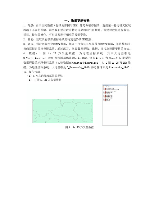
一、数据更新变换1.背景:由于空间数据(包括地形图与DEM)都是分幅存储的,造成某一特定研究区域跨越了不同的图幅。
而当我们要获取有特定边界的研究区域时,就要对数据进行裁切、拼接、提取等操作,有时还要进行相应的投影变换。
2.目的:获取具有投影坐标系统的特定边界的DEM数据。
3.要求:通过两幅给定的DEM数据,提取出白水县县界范围内的DEM数据,并将数据转换成高斯克吕格投影系统。
通过练习,掌握数据提取、裁切、拼接及投影变换的方法。
4.数据:1幅1:25万矢量数据,为地理坐标系统,其中大地基准是D_North_American_1927,参考椭球体是Clarke 1866,这是Arcgis为Shapefile类型的数据假设的地理坐标系统(实验数据在Chapter4/Exercise1中)。
2幅1:25万DEM数据,为地理坐标系统,大地基准是D_Krasovsky_1940,参考椭球体是Krasovsky_1940。
5.操作步骤:(1)白水县的行政范围的提取1)打开1:25万矢量数据图1 1:25万矢量数据2)利用Analysis Tools工具箱,Extract工具集中的Select工具,依据“name”字段,即SQL 表达式设置为“"NAME" = '白水县'”,提取出白水县图2:select对话框图3:query builder对话框A. 展开Analysis Tools工具箱,打开Extract工具集,双击Select,打开Select对话框。
B. 在Input Features文本框中选择输入“E:/ChP4/Ex1/Vector”矢量数据。
C. 在Output Feature Class文本框键入输出的数据的路径与名称“E:/ChP4/Ex1/vector_Select”。
D. 单击Expression可选文本框旁边的按钮,打开Query Builder对话框,设置SQL表达式“"NAME" = '白水县'”。

Workshop 1bSubstructures: Surface Mount AnalysisKeywords VersionNote: This workshop provides instructions in terms of the Abaqus Keywords interface. If you wish to use the Abaqus GUI interface instead, please see the “Interactive” version of these instructions.Please complete either the Keywords or Interactive version of this workshop.GoalsWhen you complete this workshop, you will be able to:•Define a substructure model (for both generation and usage).•Use shared nodes to connect the generation and usage models•Use amplitude curves to define a complete thermal cycle within a single analysis stepProblem descriptionLow-cycle fatigue is a common failure mechanism in solder joints of surface mount assemblies in the electronic packaging industry. Cyclic thermal loading combined with differences in thermal expansion properties for the various components of the assembly lead to stress reversals and the accumulation of inelastic strain in the joints. Predictions of fatigue life in solder joints require a thorough understanding of the deformation and failure mechanisms of the solder alloy and an accurate calculation of the stresses and strains in the joint.A structural model of one-quarter of a 100-pin plastic quad flat pack (PQFP), shown in Figure W1b–1, consists of a printed circuit board (PCB), an electronic chip, bond pads, solder joints, and gullwing leads. Symmetry boundary conditions are imposed on the appropriate faces of the PCB and the electronic chip. The assembly is constrained vertically at the point on the bottom of the PCB at the intersection of the two symmetry planes. The PQFP is subject to a thermal loading cycle that consists of heating the PQFP uniformly from 0°C to 125°C, holding at 125°C, cooling uniformly from 125°C to 0°C, and holding at 0°C. Heating and cooling are performed linearly over 1 minute, while holding periods are 15 minutes in duration. The PQFP is assumed to be stress-free initially at a reference temperature of 0°C.W1b.2 The components of the PQFP have dissimilar coefficients of thermal expansion (CTEs). The greatest thermal mismatch occurs between the electronic chip and the PCB and between the solder joints and the leads. The solder joints and the leads near the corner of the PQFP experience the highest deformations since they are farthest from the center of the assembly. Because failure is most likely to occur in this area, these joints and leads are more finely meshed (see Figure W1b–2) so that sufficiently accurate stresses and strains can be calculated. The elastic behavior of the solder is modeled with a temperature-dependent modulus of elasticity. The solder’s inelastic response is characterized with a double power-law creep model (see Knowledge Base ArticleQA00000008827 for details of this model). The other components of the PQFP are considered to behave as temperature-independent, linear elastic materials.The problem is simplified by assuming that all but the corner solder joints are composed of temperature-independent, linear elastic materials. Based on the assumption that the bulk of the PQFP behaves strictly linearly, this portion of the assembly can be treated as a single linear substructure. The nonlinear behavior of the corner legs is modeled with “regular” elements (those outside the substructure). The analysis consists of a single substructure generation step and three cycles of thermal loading.The units used in this problem are N, mm, sec, and degrees Celsius.Figure W1b–1 100-pin plastic quad flat pack.W1b.3Figure W1b–2 Close-up view of refined mesh for corner legs.Preliminaries1.Enter the working directory for this workshop:../substructuring/keywords/mountThe files w_surface_mount_gen.inp and w_surface_mount.inp contain the models that you will use in this workshop.Substructure generation1.Open the input file named w_surface_mount_gen.inp in a text editor.2.Apply an initial temperature to the set NALL. Set the initial temperature to zero:*INITIAL CONDITIONS, TYPE=TEMPERATURENALL, 0.3.Define a substructure generation step. Set the substructure identifier to 1 andsuppress the evaluation of the recovery matrix:*STEP*SUBSTRUCTURE GENERATE, TYPE=Z1, RECOVERY MATRIX=NOW1b.4 4.In the substructure generation step, retain all nodal degrees of freedom for the setRETAINED:*RETAINED NODAL DOFSRETAINED, 1, 65.In the substructure generation step, apply the following displacement boundaryconditions:•For the set XSYMM: fix degree of freedom 1•For the set YSYMM: fix degree of freedom 2•For the set PINZ: fix degree of freedom 3*BOUNDARYXSYMM, 1, 1YSYMM, 2, 2PINZ, 3, 36.Include the following substructure load case in the substructure generation step:*SUBSTRUCTURE LOAD CASE, NAME=TEMP*TEMPERATURENALL, 1.07.End the step definition:*END STEP8.Save the input file and submit the job for analysis in order to generate thesubstructure files. Monitor the progress of the job and address any warning or error messages if necessary.W1b.5 Substructure usage1.Once the job completes, open the input file named w_surface_mount.inp in atext editor. You will import the substructure generated previously to assemble the model shown in Figure W1b–2.2.Delete all keyword options related to parts and assemblies:*PART*END PART*INSTANCE*END INSTANCE*ASSEMBLY*END ASSEMBLY3.Modify the surface names used with the tied contact pair definition to remove thereference to the instance name:*CONTACT PAIR, ...NLEAD1, SPACK1NLEAD2, SPACK2NPAD1, SBOARD1NPAD2, SBOARD2e the ELEMENT and *SUBSTRUCTURE PROPERTY options to place thesubstructure in your model. For the substructure use an element label that does not conflict with any of the other elements currently defined in the model (e.g., labelthe substructure element 1). The connectivity list for the substructure is found inthe predefined node set named CHPBRD (simply copy-and-paste when definingthe element connectivity):*ELEMENT, TYPE=Z1, FILE=w_surface_mount_gen, ELSET=CHPBRD1, 1451,1452,1453,1454,...::...,8018,8040,8041*SUBSTRUCTURE PROPERTY,ELSET=CHPBRDW1b.6 5.The time history of the temperature will be varied according the curve shown inFigure W1b–3. Recall that the heating and cooling are performed linearly over 1 minute, while holding periods are 15 minutes in duration.Figure W1b–3 Temperature history in each cycle.Thus, define a tabular amplitude function named TEMP-AMP as shown below.Note that the time scale used is in seconds.*AMPLITUDE, NAME=TEMP-AMP0., 0., 60., 1., 960., 1., 1020., 0.1920., 0.6.Apply an initial temperature to the set NALL. Set the initial temperature to zero:*INITIAL CONDITIONS, TYPE=TEMPERATURENALL, 0.W1b.77.Define a VISCO step named CYCLE-1.•Set the NLGEOM parameter equal to YES.•Set the time period to 1920 sec, the initial increment size to 1 sec, the minimum increment size to 1e-7 sec, and the maximum increment sizeto 75 sec.•In addition, set the creep error tolerance to 0.001.*STEP, NAME=CYCLE-1, NLGEOM=YES*VISCO, CETOL=0.0011., 1920., 1E-07, 75.8.Modify the predefined temperature field so that the reference temperature is set to125 and the amplitude curve is set to TEMP-AMP:*TEMPERATURE, AMPLITUDE=TEMP-AMPNALL, 125.9.Create a substructure load in the first step. Set the magnitude multiplier to 125and the amplitude curve to TEMP-AMP:*SLOAD, AMPLITUDE=TEMP-AMPCHPBRD, TEMP, 125.10.Modify the default field output request to include the element temperature:*OUTPUT, FIELD, VARIABLE=PRESELECT*ELEMENT OUTPUTTEMP11.Modify the default history output request to set the output frequency to every 60units of time:*OUTPUT, HISTORY, VARIABLE=PRESELECT, TIME INTERVAL=60.With this setting, history output will be written at exact times. Since the timepoints in the amplitude curve are multiples of 60, this ensures that the time points in the amplitude curve will be evaluated exactly with the analysis step. Thisfacilitates the use of the amplitude definition for the purpose of defining thecomplete thermal cycle within one analysis step.W1b.8 12.End the step definition:*END STEP13.Create two additional VISCO steps similar to the first. Name them CYCLE-2 andCYCLE-3, respectively:*STEP, NAME=CYCLE-2*VISCO, CETOL=0.0011., 1920., 1E-07, 75.***SLOAD, AMPLITUDE=TEMP-AMPCHPBRD, TEMP, 125.***TEMPERATURE, AMPLITUDE=TEMP-AMPNALL, 125.***END STEP***STEP, NAME=CYCLE-3*VISCO, CETOL=0.0011., 1920., 1E-07, 75.***SLOAD, AMPLITUDE=TEMP-AMPCHPBRD, TEMP, 125.***TEMPERATURE, AMPLITUDE=TEMP-AMPNALL, 125.***END STEP14.Save the input file and submit the job for analysis in order to generate thesubstructure files. Monitor the progress of the job and address any warning or error messages if necessary.W1b.9 Postprocessing1.Once the job completes, open w_surface_mount.odb in Abaqus/Viewer.2.Examine the deformation history in the corner legs. The deformation at the end ofthe first holding period at 125 C is shown in Figure W1b–4. Note that thedeformation scale factor is set to 20 in this figure.Figure W1b–4 Deformation during first holding period at 125°C (step time = 960) Note that the larger CTE of the PCB with respect to the chip leads to an upwardcurling motion of the PCB, which in turn causes stretching and twisting of eachleg.3.Contour the equivalent creep strain in the corner legs. The maximum creep strainsoccur in the toe area closest to the corner of the PQFP. The equivalent creep strain distribution in the toe area at the end of the third cycle is shown in Figure W1b–5.Tip: To create this plot, restrict the display to the element set named PART-1-1.SOLDERF.AFigure W1b–5 Equivalent creep strain in the solder joint after three thermalcycles.W1b.10 4.Examine the time history of the equivalent creep strain. The equivalent creep strainhistory at point A (indicated in Figure W1b–5) is shown in Figure W1b–6.Tip: To create this plot, extract Centroid field data for the element at the corner of the toe area.Figure W1b–6 Creep strain history at point A.As expected, there is significantly more creep strain accumulated during the first cycle, largely due to the initial twisting in the joints. The second and third cycles show similar creep response. Once the creep strain increment per cycle reaches a constant, this value can be used in a relationship, such as the Coffin-Manson equation, to estimate the fatigue life of the solder joints.W1b.115.Examine the time history of the Mises stress. The Mises stress history at point A isshown in Figure W1b–7.Figure W1b–7 Mises stress history at point A.The second and third cycles appear to be the same because the initial stress stateconditions of the second and subsequent cycles are similar. The initial dip andsubsequent peak in stress during the heating stage of the second and third cyclesare due to the combination of the initial stress state and the competing effects ofcreep relaxation and CTE mismatch between the PCB and chip.Note: Complete input files are available for your convenience. You may consult these files if you encounter difficulties following the instructions outlined here or if you wish to check your work. The input files are named w_surface_mount_gen_complete.inpw_surface_mount_complete.inpand are available using the Abaqus fetch utility.© Dassault Systèmes, 2013 Substructures and Submodeling with Abaqus。
实验八:栅格数据处理一、实验目的1、掌握栅格数据进行裁切、拼接、提取等操作;2、掌握投影变换方法。
二、实验准备数据准备:1幅1:25万矢量数据(Vector),为白水县的行政范围。
地理坐标系统,其中大地基准是D_North_American_1927,参考椭球体是Clarke 1866。
2幅1:25万DEM数据(DEM1和DEM2)。
地理坐标系统,其中大地基准是D_Krasovsky_1940,参考椭球体是Krasovsky_1940。
软件准备:ArcGIS Desktop9.x,ArcCatalog三、实验内容白水县跨两个DEM图幅,提取出白水县的DEM数据,并将数据转换成高斯克吕格投影系统。
获取具有投影坐标系统的特定边界DEM数据。
工作流程如图1所示。
图1 工作流程四、实验步骤(1)白水县行政范围的提取1) 打开1:25万矢量数据(图2)。
2) 利用Analysis Tools 工具箱,Extract 工具集中的Select 工具,依据“name ”字段,即SQL 表达式设置为“"NAME" = '白水县'”,提取出白水县地图数据(图3)。
A 展开Analysis Tools 工具箱,打开Extract 工具集,双击Select ,打开Select 对话框。
B 在Input Features 文本框中选择输入“E :/ChP4/Ex1/Vector ”矢量数据。
C 在Output Feature Class 文本框键入输出的数据的路径与名称“E :/ChP4/Ex1/vector_Select ”。
D单击Expression 可选文本框旁边的按钮,打开Query Builder 对话框,设置SQL 表达式“"NAME" = '白水县'”。
E单击OK 按钮,完成操作。
图2 原始矢量数据(2) D EM 数据拼接1) 打开白水县横跨的两幅DEM 数据,DEM1和DEM2(图4)。
DESIGN OF HEAT EXCHANGER FOR HEAT RECOVERY IN CHP SYSTEMSABSTRACTThe objective of this research is to review issues related to the design of heat recovery unit in Combined Heat and Power (CHP) systems. To meet specific needs of CHP systems, configurations can be altered to affect different factors of the design. Before the design process can begin, product specifications, such as steam or water pressures and temperatures, and equipment, such as absorption chillers and heat exchangers, need to be identified and defined. The Energy Engineering Laboratory of the Mechanical Engineering Department of the University of Louisiana at Lafayette and the Louisiana Industrial Assessment Center has been donated an 800kW diesel turbine and a 100 ton absorption chiller from industries. This equipment needs to be integrated with a heat exchanger to work as a Combined Heat and Power system for the University which will supplement the chilled water supply and electricity. The design constraints of the heat recovery unit are the specifications of the turbine and the chiller which cannot be altered.INTRODUCTIONCombined Heat and Power (CHP), also known as cogeneration, is a way to generate power and heat simultaneously and use the heat generated in the process for various purposes. While the cogenerated power in mechanical or electrical energy can be either totally consumed in an industrial plant or exported to a utility grid, the recovered heat obtained from the thermal energy in exhaust streams of power generating equipment is used to operate equipment such as absorption chillers, desiccant dehumidifiers, or heat recovery equipment for producing steam or hot water or for space and/or process cooling, heating, or controlling humidity. Based on the equipment used, CHP is also known by other acronyms such as CHPB (Cooling Heating and Power for Buildings), CCHP (Combined Cooling Heating and Power), BCHP (Building Cooling Heating and Power) and IES (Integrated Energy Systems). CHP systems are much more efficient than producing electric and thermal power separately. According to the Commercial Buildings Energy Consumption Survey, 1995 [14], there were 4.6 million commercial buildings in the United States. These buildings consumed 5.3 quads of energy, about half of which was in the form of electricity. Analysis of survey data shows that CHP meets only 3.8% of the total energy needs of the commercial sector. Despite the growing energy needs, the average efficiency of power generation has remained 33% since 1960 and the average overall efficiency of generating heat and electricity using conventional methods is around 47%. And with the increase in prices in both electricity and natural gas, the need for setting up more CHP plants remains a pressing issue. CHP is known to reduce fuel costs by about 27% [15] CO released into the atmosphere. The objective of this research is to review issues related to the design of heat recovery unit in Combined Heat and Power (CHP) systems. To meet specific needs of CHP systems, configurations can be altered to affect differentfactors of the design. Before the design process can begin, product specifications, such as steam or water pressures and temperatures, and equipment, such as absorption chillers and heat exchangers, need to be identified and defined.The Mechanical Engineering Department and the Industrial Assessment Center at the University of Louisiana Lafayette has been donated an 800kW diesel turbine and a 100 ton absorption chiller from industries. This equipment needs to be integrated to work as a Combined Heat and Power system for the University which will supplement the chilled water supply and electricity. The design constraints of the heat recovery unit are the specifications of the turbine and the chiller which cannot be altered.Integrating equipment to form a CHP system generally does not always present the best solution. In our case study, the absorption chiller is not able to utilize all of the waste heat from the turbine exhaust. This is because the capacity of the chiller is too small as compared to the turbine capacity. However, the need for extra space conditioning in the buildings considered remains an issue which can be resolved through the use of this CHP system. BACKGROUND LITERATUREThe decision of setting up a CHP system involves a huge investment. Before plunging into one, any industry, commercial building or facility owner weighs it against the option of conventional generation. A dynamic stochastic model has been developed that compares the decision of an irreversible investment in a cogeneration system with that of investing in a conventional heat generation system such as steam boiler combined with the option of purchasing all the electricity from the grid [21]. This model is applied theoretically based on exempts. Keeping in mind factors such as rising emissions, and the availability and security of electricity supply, the benefits of a combined heat and power system are many.CHP systems demand that the performance of the system be well tested. The effects of various parameters such as the ambient temperature, inlet turbine temperature, compressor pressure ratio and gas turbine combustion efficiency are investigated on the performance of the CHP system and determines of each of these parameters [1]. Five major areas where CHP systems can be optimized in order to maximize profits have been identified as optimization of heat to power ratio, equipment selection, economic dispatch, intelligent performance monitoring and maintenance optimization [6].Many commercial buildings such as universities and hospitals have installed CHP systems for meeting their growing energy needs. Before the University of Dundee installed a 3 MW CHP system, first the objectives for setting up a cogeneration system in the university were laid and then accordingly the equipment was selected. Considerations for compatibility of the new CHP setup with the existing district heating plant were taken care by some alterations in pipe work so that neither system could impose any operational constraints on the other [5]. Louisiana State University installed a CHP system by contracting it to Sempra EnergyServices to meet the increase in chilled water and steam demands. The new cogeneration system was linked with the existing central power plant to supplement chilled water and steam supply. This project saves the university $ 4.7 million each year in energy costs alone and 2,200 emissions are equivalent to 530 annual vehicular emissions.Another example of a commercial CHP set-up is the Mississippi Baptist Medical Center. First the energy requirement of the hospital was assessed and the potential savings that a CHP system would generate [10]. CHP applications are not limited to the industrial and commercial sector alone. CHP systems on a micro-scale have been studied for use in residential applications. The cost of UK residential energy demand is calculated and a study is performed that compares the operating cost for the following three micro CHP technologies: Sterling engine, gas engine, and solid oxide fuel cell (SOFC) for use in homes [9].The search for different types of fuel cells in residential homes finds that a dominant cost effective design of fuel cell use in micro – CHP exists that is quickly emerging [3]. However fuel cells face competition from alternate energy products that are already in the market. Use of alternate energy such as biomass combined with natural gas has been tested for CHP applications where biomass is used as an external combustor by providing heat to partially reform the natural gas feed [16]. A similar study was preformed where solid municipal waste is integrated with natural gas fired combustion cycle for use in a waste-to-energy system which is coupled with a heat recovery steam generator that drives a steam turbine [4]. SYSTEM DESIGN CONSIDERATIONSIntegration of a CHP system is generally at two levels: the system level and the component level. Certain trade-offs between the component level metrics and system level metrics are required to achieve optimal integrated cooling, heating and power performance [18]. All CHP systems comprise mainly of three components, a power generating equipment or a turbine, a heat recovery unit and a cooling device such as an absorption chiller.There are various parameters that need to be considered at the design stage of a CHP project. For instance, the chiller efficiency together with the plant size and the electric consumption of cooling towers and condenser water pumps are analyzed to achieve the overall system design [20]. Absorption chillers work great with micro turbines. A good example is the Rolex Reality building in New York, where a 150 kW unit is hooked up with an absorption chiller that provides chilled water. An advantage of absorption chillers is that they don’t require any permits or emission treatment [2]Exhaust gas at 800°F comes out of the turbine at a flow rate of 48,880 lbs/h [7]. One important constraint during the design of the CHP system was to control the final temperature of this exhaust gas. This meant utilizing as much heat as required from the exhaust gas and subsequently bringing down the exit temperature. After running different iterations on temperature calculations, it was decided to divert 35% of the exhaust air to the heat exchanger whilethe remaining 65% is directed to go up the stack. This is achieved by using a diverter damper. In addition, diverting 35% of the gas relieves the problem of back pressure build-up at the end of the turbine.A diverter valve can also used at the inlet side of the heat exchanger which would direct the exhaust gas either to the heat exchanger or out of the bypass stack. This takes care of variable loads requirement. Inside the heat exchanger, exhaust gas enter the shell side and heats up water running in the tubes which then goes to the absorption chiller. These chillers run on either steam or hot water.The absorption chiller donated to the University runs on hot water and supplies chilled water. A continuous water circuit is made to run through the chiller to take away heat from the heat input source and also from the chilled water. The chilled water from the absorption chiller is then transferred to the existing University chilling system unit or for another use.Thermally Activated DevicesThermally activated technologies (TATs) are devices that transform heat energy for useful purposed such as heating, cooling, humidity control etc. The commonly used TATs in CHP systems are absorption chillers and desiccant dehumidifiers. Absorption chiller is a highly efficient technology that uses less energy than conventional chilling equipment, and also cools buildings without the use of ozone-depleting chlorofluorocarbons (CFCs). These chillers can be powered by natural gas, steam, or waste heat.Desiccant dehumidifiers are used in space conditioning by removing humidity. By dehumidifying the air, the chilling load on the AC equipment is reduced and the atmosphere becomes much more comfortable. Hot air coming from an air-to-air heat exchanger removes water from the desiccant wheel thereby regenerating it for further dehumidification. This makes them useful in CHP systems as they utilize the waste heat.An absorption chiller is mechanical equipment that provides cooling to buildings through chilled water. The main underlying principle behind the working of an absorption chiller is that it uses heat energy as input, instead of mechanical energy.Though the idea of using heat energy to obtain chilled water seems to be highly paradoxical, the absorption chiller is a highly efficient technology and cost effective in facilities which have significant heating loads. Moreover, unlike electrical chillers, absorption chillers cool buildings without using ozone-depleting chlorofluorocarbons (CFCs). These chillers can be powered by natural gas, steam or waste heat.Absorption chiller systems are classified in the following two ways:1. By the number of generators.i) Single effect chiller –this type of chiller, as the name suggests, uses one generator and the heat released during the absorption of the refrigerant back into the solution is rejected to the environment.ii) Double effect chiller –this chiller uses two generators paired with a single condenser, evaporator and absorber. Some of the heat released during the absorption process is used to generate more refrigerant vapor thereby increasing the chiller’s efficiency as more vapor is generated per unit heat or fuel input. A double effect chiller requires a higher temperature heat input to operate and therefore its use in CHP systems is limited by the type of electrical generation equipment it can be used with.iii) Triple effect chiller –this has three generators and even higher efficiency than a double effect chiller. As they require even higher heat input temperatures, the material choice and the absorbent/refrigerant combination is limited.2. By type of input:i) Indirect-fired absorption chillers –they use steam, hot water, or hot gases from a boiler, turbine, engine generator or fuel cell as a primary power input. Indirect-fired absorption chillers fit well into the CHP schemes where they increase the efficiency by utilizing the otherwise waste heat and producing chilled water from it.ii) Direct-fired absorption chillers –they contain burners which use fuel such as natural gas. Heat rejected from these chillers is used to provide hot water or dehumidify air by regenerating the desiccant wheel.An absorption cycle is a process which uses two fluids and some heat input to produce the refrigeration effect as compared to electrical input in a vapor compression cycle in the more familiar electrical chiller. Although both the absorption cycle and the vapor compression cycle accomplish heat removal by the evaporation of a refrigerant at a low pressure and the rejection of heat by the condensation of refrigerant at a higher pressure, the method of creating the pressure difference and circulating the refrigerant remains the primary difference between the two. The vapor compression cycle uses a mechanical compressor that creates the pressure difference necessary to circulate the refrigerant, while the same is achieved by using a secondary fluid or an absorbent in the absorption cycle [11].The primary working fluids ammonia and water in the vapor compression cycle with ammonia acting as the refrigerant and water as the absorbent are replaced by lithium bromide (LiBr) as the absorbent and water (H2O) as the refrigerant in the absorption cycle. The process occurs in two shells - the upper shell consisting of the generator and the condenser and the lower shell consisting of the evaporator and the absorber.Heat is supplied to the LiBr/H2O solution through the generator causing the refrigerant (water) to be boiled out of the solution, as in a distillation process. The resulting water vapor passes into the condenser where it is condensed back into the liquid state using a condensing medium. The water then enters the evaporator where actual cooling takes place as water is passes over tubes containing the fluid to be cooled.Heat ExchangerA very low pressure is maintained in the absorber-evaporator shell, causing the water to boil at a very low temperature. This results in water absorbing heat from the medium to be cooled and thereby lowering its temperature. The heated low pressure vapor then returns to the absorber where it mixes with the LiBr/H2O solution low in water content. Due to the solution’s low water content, vapor gets easily absorbed resulting in a weaker LiBr/H2O solution. This weak solution is pumped back to the generator where the process repeats itself.The heat recovery steam generator (HRSG) is primarily a boiler which generates steam from the waste heat of a turbine to drive a steam turbine. The heat recovery boiler design for cogeneration process applications covers many parameters. The boiler could be designed as a fire-tube, water tube or combination type. Further for each of these parameters, there is a variety of tube sizes and fin configurations. For a given boiler, a simplified method that determines the boiler performance has been developed [8].The shell and tube heat exchanger is the most common and widely used heat exchanger in different industrial applications [13]. It is compared to a classic instrument in a concert playing all the important nodes in different complex system set-ups and can be improved by using helical baffles. There are other ways to augment the heat transfer in a shell and tube exchanger such as through the use of wall-radiation [25].The design of a shell and tube heat exchanger fora combined heat and power system basically involves determining its size or geometry by predicting the overall heat transfer coefficient (U). The process of obtaining the heat transfer coefficient values is obtained from literature by correlating results from previous findings in the determination of heat exchanger designs.This involves listing assumptions at the beginning of the procedure, obtaining fluid properties, calculation of Reynolds number and the flow area to obtain the shell and tube sizes. Once U is calculated, the heat balances are calculated. This study also compares the theoretical U values with the actual experimental ones to prove the theoretical assumptions and to obtain the optimum design model [18].A mathematical simulation for the transient heat exchange of a shell and tube heat exchanger based on energy conservation and mass balance can be used to measure the performance. The design of the heat exchanger is optimized with the objective function being the total entropy generation rate considering the heat transfer and the flow resistance [20].Once a heat exchanger is designed, a total cost equation for the heat exchanger operation is deduced. Based on this, a program is developed for the optimal selection of shell-tube heat exchanger [24].The heat exchanger to be used in the CHP system in the end needs to be tested for its performance. A heat recovery module f orcogeneration is tested before use for CHP application through a microprocessor based control system to present the system design and performance data [19].The basis of a CHP system lies in efficiently capturing thermal energy and using it effectively. Generally in CHP systems, the exhaust gas from the prime mover is ducted to a heat exchanger to recover the thermal energy in the gas. The commonly used heat recovery systems are heat exchangers and Heat Recovery Steam Generators depending on whether hot water or steam is required.The heat exchanger is typically an air-to-water kind where the exhaust gas flows over some form of tube and fin heat exchange surface and the heat from the exhaust gas is transferred to make hot water. Sometimes, a diverter or a flapper damper is used to maintain a specific design temperature of the hot water or steam generation rate by regulating the exhaust flow through the heat exchanger.The HRSG is essentially a boiler that captures the heat from the exhaust of a prime mover such as a combustion turbine, gas or diesel engine to make steam. Water is pumped and circulated through the tubes which are heated by exhaust gases at temperatures ranging from 800°F to 1200°F. The water can then be held under high pressure to temperatures of 370°F or higher to produce high pressure steam [21].The Delaware method is a rating method regarded as the most suitable open-literature available for evaluating shell side performance and involves the calculation of the overall heat transfer coefficient and the pressure drops on both the shell and tube side for single-phase fluids [12]. This method can be used only when the flow rates, inlet and outlet temperatures, pressures and other physical properties of both the fluids and a minimum set of geometrical properties of the shell and tube are known. Emission ControlEmission control technologies are used in the CHP systems to remove SO2 (sulphur dioxide), SO3 (sulphur trioxide) NOx (nitrous oxide) and other particulate matter present in the exhaust of a prime mover. Some common emission control technologies are:1、Diesel Oxidation Catalyst (DOC) –They are know to reduce emissions of carbon monoxide by 70 percent, hydrocarbons by 60 percent, and particulate matter by 25 percent (Emissions Control : CHP Technologies Gulf Coast CHP 2007) when used with the ultra-low sulfur diesel (ULSD) fuel. Reductions are also significant with the use of regular diesel fuel.2、Diesel Particulate Filter (DPF) - DPF can reduce emissions of carbon monoxide, hydrocarbons, and particulate matter by approximately 90 to 95 percent (Emissions Control : CHP Technologies Gulf Coast CHP 2007). However, DPF are used only in conjunction with ultra-low sulfur diesel (ULSD) fuel.3、Exhaust Gas Recirculation (EGR) – They have a great potential for reducing NOx emissions.4、Selective Catalytic Reduction (SCR) –SCR cuts down high levels of NOx by reducing NOx to nitrogen (N2) and oxygen (O2).5、NOx absorbers –catalysts are used which adsorb NOx in the exhaust gas and dissociates it to nitrogen.CONCLUSIONSThe various components needed in a CHP system have been presented. Important parameters such as the mass flow rates of the exhaust gas and water can then be defined. The CHP system has been integrated by the use of a heat recovery unit, the design of which has been discussed. A shell and tube configuration is commonly selected based on literature survey. The pressure drops at both the shell and the tube side can be calculated after the exchanger has been sized.Integrating equipment to form a CHP system generally does not always present the best solution. In our case study, the absorption chiller is not able to utilize all of the waste heat from the turbine exhaust. Approximately 65% goes is left to go out the stack. This is because the capacity of the chiller is too small as compared to the turbine capacity. However, the need for extra space conditioning in the buildings considered remains an issue which can be resolved through the use of this CHP system.The heat exchanger designed can either be constructed following the TEMA standards or it can be built and purchased from an industrial facility. The design that is used is based on the methodology of the Bell-Delaware method and the approach is purely theoretical, so the sizing may be slightly different in industrial design. Also the manufacturing feasibility needs to be checked.After the heat exchanger is constructed, the CHP equipment can be hooked together. Again since the available equipment is integrated to work as a system, the efficiency of the CHP system needs to be calculated. Some kind of co ntrol module needs to be developed that can monitor the performance of the entire system. Finally, the cost of running the set-up needs to be determined along with the air-conditioning requirements.。
How to carbon footprint your products, identify hotspots and reduce emissions in yoursupply chainThe Guide to PAS 2050:2011The Guide toPAS2050:2011How to carbon footprint your products, identifyhotspots and reduceemissions in yoursupply chainAcknowledgementsThe development of this Guide was co-sponsored by:Defra (Department for Environment, Food and Rural Affairs)DECC (Department of Energy and Climate Change)BIS (Department for Business, Innovation and Skills)Acknowledgement is given to ERM who authored this Guide. ERM has completed over 1,000 carbon footprints across more than 50 sectors and provides carbon footprinting and carbon reduction services to both UK and international clients. Acknowledgement is also given to the following organizations who assisted in its development:ADAS UK LimitedDefraFood and Drink FederationInstitute of Environmental Management and AssessmentCarbon TrustFirst published in the UK in 2011byBSI389 Chiswick High RoadLondon W4 4AL© British Standards Institution 2011All rights reserved. Except as permitted under the Copyright, Designs and Patents Act 1988, no part of thispublication may be reproduced, stored in a retrieval system or transmitted in any form or by any means –electronic, photocopying, recording or otherwise – without prior permission in writing from the publisher.Whilst every care has been taken in developing and compiling this publication, BSI accepts no liability forany loss or damage caused, arising directly or indirectly in connection with reliance on its contents exceptto the extent that such liability may not be excluded in law.While every effort has been made to trace all copyright holders, anyone claiming copyright should get intouch with the BSI at the above address.BSI has no responsibility for the persistence or accuracy of URLs for external or third-party internet websitesreferred to in this book, and does not guarantee that any content on such websites is, or will remain,accurate or appropriate.The right of ERM to be identified as the author of this Work have been asserted by the authors inaccordance with sections 77 and 78 of the Copyright, Designs and Patents Act 1988.T ypeset in Futura by Helius – Printed in Great Britain by Berforts. British Library Cataloguing in Publication DataA catalogue record for this book is available from the British LibraryISBN 978-0-580-77432-4Introduction . . . . . . . . . . . . . . . . . . . . . . . . . . . . . . . . . . . . . . . . . . . . . . . . . . . . . .1What is PAS 2050? . . . . . . . . . . . . . . . . . . . . . . . . . . . . . . . . . . . . . . . . . . . . .1Why should I use PAS 2050? . . . . . . . . . . . . . . . . . . . . . . . . . . . . . . . . . . . . . .1Why this Guide? . . . . . . . . . . . . . . . . . . . . . . . . . . . . . . . . . . . . . . . . . . . . . . .2The 2011 revision of PAS 2050 . . . . . . . . . . . . . . . . . . . . . . . . . . . . . . . . . . . .2Making product carbon footprinting work in practice . . . . . . . . . . . . . . . . . . . . .3The stepwise footprinting process . . . . . . . . . . . . . . . . . . . . . . . . . . . . . . . . . . .4Step 1. Scoping . . . . . . . . . . . . . . . . . . . . . . . . . . . . . . . . . . . . . . . . . . . . . . . . . . .51.1. Describe the product to be assessed and the unit of analysis . . . . . . . . . . . .51.2. Draw a map of the product life cycle . . . . . . . . . . . . . . . . . . . . . . . . . . . . .61.3. Agree and record the system boundary of the study . . . . . . . . . . . . . . . . . .71.4. Prioritize data collection activities . . . . . . . . . . . . . . . . . . . . . . . . . . . . . .12Step 2. Data collection . . . . . . . . . . . . . . . . . . . . . . . . . . . . . . . . . . . . . . . . . . . . .13Types of data . . . . . . . . . . . . . . . . . . . . . . . . . . . . . . . . . . . . . . . . . . . . . . . .132.1. Draw up a data collection plan . . . . . . . . . . . . . . . . . . . . . . . . . . . . . . . .142.2. Engaging suppliers to collect primary data . . . . . . . . . . . . . . . . . . . . . . . .142.3. Collecting and using secondary data . . . . . . . . . . . . . . . . . . . . . . . . . . . .162.4. Collecting data for ‘downstream’ activities . . . . . . . . . . . . . . . . . . . . . . . .182.5. Assessing and recording data quality . . . . . . . . . . . . . . . . . . . . . . . . . . . .19Step 3. Footprint calculations . . . . . . . . . . . . . . . . . . . . . . . . . . . . . . . . . . . . . . . .213.1. General calculation process . . . . . . . . . . . . . . . . . . . . . . . . . . . . . . . . . .213.2. Calculations for specific aspects of the footprint . . . . . . . . . . . . . . . . . . . .30Step4. Interpreting footprint results and driving reductions . . . . . . . . . . . . . . . . . . .424.1. Understanding carbon footprint results . . . . . . . . . . . . . . . . . . . . . . . . . . .42ContentsContents4.2. How certain can I be about the footprint and hotspots? . . . . . . . . . . . . . . .434.3. Recording the footprint . . . . . . . . . . . . . . . . . . . . . . . . . . . . . . . . . . . . . .444.4. How can I use footprinting to drive reductions? . . . . . . . . . . . . . . . . . . . .45 Annex A. Further examples of functional units . . . . . . . . . . . . . . . . . . . . . . . . . . . . .48 Annex B. Setting functional units and boundaries for services . . . . . . . . . . . . . . . . . .49 Annex C. Orange juice example: data prioritization . . . . . . . . . . . . . . . . . . . . . . . .51 Annex D. Primary data collection tips and templates . . . . . . . . . . . . . . . . . . . . . . . .59 Annex E. Sampling approaches . . . . . . . . . . . . . . . . . . . . . . . . . . . . . . . . . . . . . . .64 Annex F. A data quality assessment example . . . . . . . . . . . . . . . . . . . . . . . . . . . . . .66 Annex G. Biogenic carbon accounting . . . . . . . . . . . . . . . . . . . . . . . . . . . . . . . . . .70 Annex H. Worked CHP example . . . . . . . . . . . . . . . . . . . . . . . . . . . . . . . . . . . . . . .72 Annex I. Supplementary requirements . . . . . . . . . . . . . . . . . . . . . . . . . . . . . . . . . . .741Introduction2Introductionclarification on only one, or a small number, of aspects of the calculation process. The concept of supplementary requirements is akin to ‘Product Category Rules’ (i.e. developed through ISO 140255)and ‘Product rules’ (GHG Protocol Product Standard) and may include either of these (if consistent with PAS 2050).This symbol is used in this Guide to denote where you might be able to usefully refer to supplementaryrequirement documents for further clarity or information.Before you begin to carry out your assessment, look to see if there are supplementary requirements that may help you assess the emissions associated with your product. Where they exist they should always be used.If there are no supplementary requirements for your sector, check to see whether other rules or guidance may be applicable.6)If not, you may even want to consider starting to develop supplementary requirements within your industry.For further discussion of supplementary requirements,see Annex I.The Guide to PAS 2050:20113Making product carbonfootprinting work in practiceProduct carbon footprinting should be used as a practical tool that is tailored to the needs of your organization.It can be used to identify the main sources of emissions for all types of goods and services, from oranges to nappies and from bank accounts to hospitality.Consideration of the goal/objectives of a carbon footprint study is of paramount importance, to ensure that it will deliver the information that you need. In assessing your own organization's needs, consider the following:•Your core business priorities.How could an in-depthunderstanding of the wider GHG impacts, risks and opportunities of goods and services support your strategy/business priorities? Are any products, supply chains or markets particular priorities? What are the expectations of your customers and investors?•Judicial selection of products.Identify the productsthat make most sense to assess and improve, e.g. the top-five best sellers or top-three new designs. Decide where you want to focus your attention, bearing in mind that you cannot do everything at once.•The intended audience for a study. This affectsthe degree of accuracy and resolution needed. A footprint analysis to be used to identify opportunities for reduction can be undertaken efficiently and at a high level initially, to be built on as needed. For external claims, gaining assurance is best practice,and a rigorous approach to data collection will need to be demonstrated.•Your timescale. How does this process fit in withyour product management cycle? Decide how much5)ISO 14025:2006 Environmental labels and declarations – T ype III environmental declarations – Principles and procedures.6)For example, see the PCR library at .tw/about/index.asp.Introduction 45ScopingStep IScoping is the most important step when undertakingany product carbon footprint study. It ensures that theright amount of effort is spent in getting the right datafrom the right places to achieve robust results in themost efficient manner possible.There are four main stages to scoping, and they arebest undertaken sequentially.Step I: Scoping 6‘downstream’ of your activities are not overlooked,such as recyclability at end-of-life, or potential to influence use phase emissions.For each stage on the process map:•provide a description of the activity to aid with datacollection•identify the geographic location of each distinct stepwhere possible•include all transport and storage steps between stages.An example for orange juice is shown in Figure 1.1.3. Agree and record the system boundary of the studyOnce the process map is complete, it can be used to help identify which parts of the overall system will, and will not, be included in the assessment.As an output from this scoping stage, you should clearly document and record the ‘system boundary’ in terms of:•a list of all included life cycle stages (e.g. rawmaterials, production, use, end-of-life)•a list of all included activities and processes within each life cycle stage•a list of all excluded activities and processes,and thesteps taken to determine their exclusion.Consider the following when setting system boundaries:•which GHG emissions and removals to include•cradle-to-gate (i.e. business-to-business) assessmentsversus cradle-to-grave (business-to-consumer)assessments•which processes and activities to include or exclude •time boundaries.In some cases, supplementary requirements maydictate the system boundary that should be used for a particular product system. Where these are compatible with PAS 2050, the system boundary set out in these documents should be used.The Guide to PAS 2050:20117Which GHG emissions and removals to include?According to PAS 2050, a carbon footprint must include all emissions of the 63 GHGs listed in the specification.These include carbon dioxide (CO 2), nitrous oxide (N 2O)and methane (CH 4), plus a wide range of halogenated hydrocarbons including CFCs, HCFCs and HFCs.Each of these types of GHG molecule is capable of storing and re-radiating a different amount of energy,and therefore makes a different contribution to global warming. The relative ‘strength’ of a GHG compared with carbon dioxide is known as its global warmingpotential (GWP), for example 25 for methane.T able 1 shows the global warming potentials and common sources of some of the most important GHGs covered under PAS 2050.Removals of carbon from the atmosphere (e.g. by plants and trees) must also be included in the assessment,except in the case of the biogenic carbon contained within food or feed products. This can be a tricky aspect of the footprint calculation process (e.g. for paper- and wood-based materials), and is a newStep I: Scoping8Figure 1: An example process map for orange juicePAS 2050 requirement. Further guidance is provided in Step 3.2, heading ‘Biogenic carbon accounting and carbon storage’, and Annex G of this Guide.A cradle-to-gate or cradle-to-grave assessment?PAS 2050 allows for two standard types of assessment (Figure 2), which are often used for different purposes:The Guide to PAS 2050:20119the carbon footprint of the product they supply. In this case, it makes sense to report emissions that occur only up to the point at which the product is transferred to the buyer. It also enables footprints to be incrementally calculated and reported across a supply chain.While useful in this context, cradle-to-gate assessments lack the completeness of a full cradle-to-graveassessment, and may miss a large proportion of the impact for certain products. For example, for energy-using products, the vast majority of the overall carbon footprint will result from the electricity used in the use phase. This impact would only be included in a cradle-to-grave assessment.Source: IPCC (2007), T able 2.14; see Clause 2.7) 100-year time horizon.Note: the GWP actually used in calculations should be the latest available from the Intergovernmental Panel on Climate Change (IPCC), and you should check this periodically.Table 1: Global warming potentials and common sources of some of the most important GHGs1.Cradle to gate – which takes into account all life cycle stages from raw material extraction up to the point at which it leaves the organization undertaking the assessment.2.Cradle to grave – which takes into account all life cycle stages from raw material extraction right up to disposal at end of life.Cradle-to-gate and cradle-to-grave assessmentsCradle-to-gate assessments are commonly used where a buyer has asked a supplier to provide information onStep I: Scoping10It is vital that at least 95 per cent of the total mass and at least 95 per cent of the total anticipated impact of the final product is being assessed. Double check this during data prioritization calculations (see Step 1.4).System boundaries for services Setting system boundaries for services, in particular, can be challenging. Some guidance on doing so is provided in Annex B.The Guide to PAS2050:2011 11Table 2: Examples of high- and low-intensity materials and processesStep I: Scoping12•Emission factors : values that convert activity dataquantities into GHG emissions – based on the ‘embodied’ emissions associated with producing materials/fuels/energy, operating transport carriers,treating wastes, etc. These are usually expressed in units of ‘kg CO 2e’ (e.g. kg CO 2e per kg of orange cultivation, per litre of diesel, per km of transport or per kg of waste to landfill), and are most often from secondary sources.Choosing between primary and secondary dataCollecting primary activity data for specific activities across the supply chain can be time consuming, and so often dictates the amount of resource needed for a footprinting study. But the use of primary data generally increases the accuracy of the carbon footprint calculated, as the numbers used in the calculation relate directly to the real-life production or provision of the product or service assessed.Secondary data are usually less accurate, as they will relate to processes only similar to the one that actually takes place, or an industry average for that process.The choice between primary and secondary data should be guided by the scoping/prioritization activitiesundertaken in Step 1, as well as the underlying PAS 2050principles of:•relevance – selection of appropriate data andmethods for the specific products•completeness – inclusion of all GHG emissions andremovals arising within the system boundary that provide a material contribution13Data collectionStep 2•consistency – applying assumptions, methods anddata in the same way throughout the assessment •accuracy – reducing bias and uncertainty as far as practical•transparency – where communicating externally,provide sufficient information.In accordance with the principles of ‘relevance’ and ‘accuracy’, primary data are generally preferred.Step 2: Data collection14Note that, while the general rule is that primary data are preferred, there are some exceptions to this; for example, the case of commodity goods (see the following box).A key first task in the data collection process is toconsider primary and secondary data needs and drawup a data collection plan.Some example data collection templates, showing both generic and tailored approaches, as well as some useful tips, are provided in Annex D.The data collection template can also be used to ask for information to assess the quality of data provided. This involves a few additional questions for each data point, which will help you to ascertain how much confidence you can have in the accuracy of the data and, consequently, the accuracy of the carbon footprint. SamplingIn some cases, a product will be produced at a large number of sites. Milk in the UK, for example, is typically supplied by a large number of small/medium-sized farms, each providing an identical product (note: as suppliers are known and constant, this is differentThe Guide to PAS2050:2011 15 from a commodity good as earlier described). In thiscase, data collection for each site could be prohibitivelytime consuming, and a sampling approach is required. Annex E provides some guidance on sampling options.As with all footprinting tasks, resources should beallocated in the most efficient manner, while giving consideration to the core PAS2050 principles earlier described.Table 3: An example data collection plan for orange juice (drinks producer collecting data)Step 2: Data collection16contained in technical reports and published studies.This category also includes cradle-to-gate carbon footprint values that your suppliers might give you in response to a data request.•Disaggregated data are most often found in lifecycle inventory (LCI) databases that list all the inputs and outputs for a given process. These detail the consumption of specific raw materials/energy carriers and individual emissions, as opposed to a summary of the total CO 2e emissions.Aggregated data/emission factor sourcesT able 4 provides a list of useful sources of easilyaccessible emission factors. These are a starting point,but are by no means a definitive list of available resources.If you are using aggregated secondary data/emission factors, be careful to check that they are fit forpurpose. For example, is the system boundary used compliant with PAS 2050 boundaries? Some useful things to check are outlined in the box on page 17.Table 4: Useful sources of emission factors – some examplesDisaggregated/inventory data sourcesA list of common life cycle inventory (LCI) databases can be found at: http://lca.jrc.ec.europa.eu/ lcainfohub/databaseList.vm.Some databases are free, whereas some charge a licence fee.•An example of a licensed database is the ecoinvent LCI database found at . This is a useful source of data for over 4,000 materials andprocesses.•Examples of free databases are the European Reference Life Cycle Database (ELCD) found athttp://lca.jrc.ec.europa.eu/lcainfohub/datasetArea.vm, and US Life Cycle Inventory Database found atThe Guide to PAS2050:2011 17 /lci/database/default.asp, bothof which contain LCI datasets for selected materialsand processes.T ypically, when using LCI databases, the inventory dataare modelled in an LCA software programme, to provide emission factors (aggregated data) that can be used ina carbon footprint. However, if needed, the values for individual emissions listed in the LCI database can beused to estimate the global warming potential withoutthe use of LCA software. Tips for using LCI data in thisway are as follows:•Copying the LCI data into a spreadsheet (e.g.Microsoft Excel) might make it easier to view andinterrogate.Step 2: Data collection18retailed in London/England/Wales) can be defined within your functional unit.RetailFor the majority of products, emissions from retail operations will represent a very small part of theoverall carbon footprint. The main source of emissions will be energy use for both lighting and refrigeration.If primary data for energy use by a retail facility are not available, emissions from retail of products stored at ambient temperatures can reasonably be assumed to be comparable to those from a warehouse (see Step 3.2, heading ‘Storage emissions’, of this Guide).Refrigerated or frozen storage at retail may represent a significant source of emissions, and so should be considered in more detail. See further information on refrigeration in Step 3.2, heading ‘Refrigeration’, of this Guide.You will typically need to consider the volume of space occupied by a product, and how long it is typically stored for at the point of sale (e.g. slow-moving items must be stored for longer, and so incur greater emissions).UseA ‘use profile’ is a description of the typical way in which a product is consumed, or of the average user requirements. For example:•a use profile for product that requires cooking willrefer to the proportion of users that will typically bake, boil or microwave the product and the amount of time required in each case•a use profile for an electrical item will refer to atypical length of time the product is used for, or a typical setting (e.g. the proportion of washing machine cycles at 30/40/60 degrees).For some products, the choices made at this stage can make a significant contribution to the footprint, and introduce considerable variability, and so require careful consideration.•Identify emissions of key GHGs. As a minimum,emissions of fossil/biogenic carbon dioxide, methane and nitrous oxide should be identified, which are the predominant GHGs in the majority of instances.However , other key GHGs, such as CFCs and HCFCs,might also be included in the inventory data.•The identified GHG emissions values can thenbe multiplied by their respective global warming potential, and the results summed to derive a ‘kg CO 2e’ emission factor that can be used in your product carbon footprint calculations.•Ideally, the quantity of all key GHGs will be identified.In practice, this can be a laborious task that might only involve very minor emissions. In this case, it should be recognized that the resulting emission factor might be an underestimate, and should be clearly labelled as such in the product carbon footprint calculations.2.4. Collecting data for ‘downstream’ activitiesDistributionIn many instances you will need to collect primary data for product distribution, if under your operational control.Distribution typically comprises transportation to a retail market and a period of storage in a distribution centre or warehouse. Specific data needs and emissions calculations for these activities are discussed in Step 3.2,headings ‘Refrigeration’ and ‘Storage emissions’, of this Guide.Whether this distribution step represents an average geography (e.g. products retailed in the UK, orEurope – taking a weighted average based on sales in different locations) or specific region (e.g. productsThe Guide to PAS2050:2011 19be assessed against the principles of PAS 2050 is presented in Annex F . Note that this example outlines only one of the ways in which you could undertake a semi-quantitative assessment to flag areas of uncertainty (and potential need for data improvement).The best-quality data should always be sought in an assessment, but is of particular importance where external communication is an ultimate goal of the study. In this case, a full data quality assessment,Step 2: Data collection20along with any accompanying assumptions or calculations, should be recorded with the product carbon footprint calculations.For internal assessments (e.g. to identify hotspots in the value chain), formal assessment/recording may not be needed, but you should ensure that differences in data quality are not unduly influencing the findings of your study (see Step 4 of this Guide for further discussionon this).Consider the examples for orange juice (Figure 3 and T able 5, and Figure 4 and T able 6), which show calculations for the first two life cycle stages.Activity data are often collected in many different formats and relating to different units (e.g. inputs and outputs for a tonne of raw material produced, or a year’s worth of production, or a hectare’s worth of production). An important next step is to balance the flows shown in21Footprint calculationsStep 3Step 3: Footprint calculations22HGV , heavy goods vehicle.aThe emissions from fertilizers and pesticides are dictated by their content of minerals or active ingredients (e.g. the proportion of fertilizer that is nitrogen or the proportion of pesticide that is anthraquinone) not the total weight.However, transport of the fertilizer or pesticide to use should be calculated based on the total weight.Figure 3: Mapping activity data – cultivation of oranges for the production of orange juiceTable 5: Example – 1hectare of orange cultivationThe Guide to PAS 2050:2011 23Table 6: Example – to produce 1tonne of concentrateFigure 4: Mapping activity data – processing of oranges for the production of orange juicethe process map so that all inputs and outputs reflect the provision of the functional unit/reference flow defined in Step 1. This can be either done within the process map itself, or in an Excel spreadsheet or other software tool.This can be the most difficult part of the calculation process. Golden rules are to:•always consider waste in the process•make calculations as transparent as possible, sothey can be traced backwards•record all assumptions and data concerns.Once the flows are balanced to reflect the functional unit, the calculation process is simple.Remember that some flows might be negative, where there are biogenic carbon removals (see Step 3.2,Step 3: Footprint calculations24heading ‘Biogenic carbon accounting and carbon storage’, and Annex H of this Guide).A simplified example for orange juice is shown inT able 7. Specific calculation aspects, such as transport,refrigerant or waste management are also discussed later in this section.The Guide to PAS2050:2011 25 Table 7: Footprint calculations for the production of a 1litre carton of orange juice (example data only)(Continued)(Continued)Table 7: Footprint calculations for the production of a 1litre carton of orange juice (example data only) (continued)Making simplifying assumptionsIt is often possible to use simplifications or estimations to streamline the carbon footprinting process. For example:•grouping all cleaning chemicals and using a generic ‘chemicals’ emission factor, estimating the quantities used•assigning a set of general assumptions for transport– e.g. 50km to waste treatment, 200km for inputs from the UK and 1,000km from central Europe.When making any simplifying assumptions it is important to make them conservative/worst case, and make sure that you record them and are able to change them if needed.In the calculation step of the footprint, it is a good idea to check and confirm that these simplified inputs or activities are not significant contributors to the footprint (e.g. >5 per cent of the footprint). If they are, you may need to go back and collect more specific information.As discussed in Step 2.5 of this Guide, the best quality (and specific) data should always be sought in anassessment, but is of particular importance whereexternal communication is an ultimate goal of the study.For both external and internal assessments, it is most important to ensure that differences in data quality are not unduly influencing the findings of your study (discussed further in Step 4 of this Guide).Co-product allocationSome processes in the life cycle of a product may yield more than one useful output (‘co-products’). For example, in the life cycle of orange juice above,the juicing of oranges yields not only orange juice but also a large volume of pulp (a low-value co-product that can be used as an animal feed) and a small amount of peel oil (a high-value essential oil that can be used as a fragrance in perfumes or household cleaners).In these cases, the input and output flows, or emissions,of the process (juicing) must be split, or ‘allocated’between the product being studied (the juice) and any co-products (the pulp and peel oil).aThis is the global warming potential (GWP) of N 2O gas – not an emission factor. The gas is released directly, and so does not need multiplying by an emission factor. It does, however need to be multiplied by its GWP of 298 to translate into CO 2equivalents (CO 2e).bLand-spreading – this is put to useful purpose, and so is a co-product, albeit with minimal value. A simple approach is to allocate this co-product zero emissions, as its relative value is very small (see Step 3.1, heading ‘Co-product allocation’, of this Guide).cThese values include removals and emissions of biogenic carbon within the packaging material. See Step 3.2,heading ‘Biogenic carbon accounting and carbon storage’, of this Guide.Table 7: Footprint calculations for the production of a 1litre carton of orange juice (example data only)(continued)。
高效分子排阻色谱法同时测定白及多糖分子量和含量李楠1,李卓2,张燕1,王虎成1,刘江云1*,蔡培烈1,2,杨世林1(1.苏州大学药学院,苏州215123;2.辽宁诺康生物制药有限责任公司,沈阳110016)摘要目的:建立同时测定白及多糖分子量和含量的高效分子排阻色谱分析方法。
方法:采用TSK-gel G4000PWXL色谱柱(10μm,7.8mmˑ300mm),流动相为纯水,流速0.6mL·min-1,柱温30ħ,示差折光检测器检测。
结果:白及多糖重均分子量的线性范围为24.17 178.0k(R2=0.9943),含量测定线性范围为8.22 20.55·mg·mL-1(R2=0.9992),分子量、含量精密度试验RSD分别为0.11%和0.96%(n=6),重复性RSD为0.28%和1.1%(n=5)。
结论:该方法简便快速,结果准确,重复性好,可作为白及多糖分子量和含量测定的有效方法。
关键词:白及多糖;分子排阻色谱(SEC);分子量;含量;中药多糖分析中图分类号:R917文献标识码:A文章编号:0254-1793(2012)10-1801-03Determination of molecular weight and content of Bletilla striataglucomannan by high performance size exclusion chromatographyLI Nan1,LI Zhuo2,ZHANG Yan1,WANG Hu-cheng1,LIU Jiang-yun1*,CAI Pei-lie1,2,YANG Shi-lin1(1.School of Pharmaceutical Science,SooChow University,Suzhou215123,China;2.Nuokang Bio-pharmaceutical Inc.,Shenyang110016,China)Abstract Objective:To develop a high performance size exclusion chromatography method for the determinationof molecular weight and content of polysaccharide from Bletilla striata.Methods:The TSK-gel G4000PWXL(10μm,7.8mmˑ300mm)column was used at30ħ,with water as the mobile phase at the flow rate of0.6mL·min-1.Refractive index detector was applied.Results:The average molecular weight of Bletilla striata polysaccha-ride ranged from24.17k to178.0k(R2=0.9943).The content of Bletilla striata polysaccharide ranged from 8.22to20.55mg·mL-1(R2=0.9992).Relative standard deviations(RSDs)of measurement precision of molec-ular weight and content were0.11%and0.96%(n=6),respectively.RSDs of the repeatability were0.28%,and 1.14%(n=5),respectively.Conclusion:The method is simple,rapid and effective for the measurement of molec-ular weight and content of Bletilla striata polysaccharides.Key words:Bletilla striata polysaccharide;size exclusion chromatography(SEC);molecular weight;content;tradi-tional medicine polysaccharide analysis白及(Bletilla striata(Thunb.)Reichb.f.)为兰科白及属植物,其干燥块茎作为传统中药,功能收敛止血、补肺、消肿生肌等,用于咯血、吐血、外伤出血、皮肤皴裂,白及多糖是其主要有效成分[1,2]。