神经网络和遗传算法中英文对照外文翻译文献

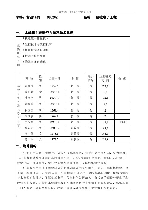
学科、专业代码 080202 名称机械电子工程一、本学科主要研究方向及学术队伍
二、培养目标
三、研究生课程学习及学分的基本要求
总学分35 分
其中公共学位课必修 2 门共 5 学分专业（或专业基础）学位课必修 5 门共13 学分
非学位课须修7 门不少于12 学分
教学实践共 2 学分必修环节：论文选题(开题报告)共 1 学分
学术活动共 1 学分
发表论文共 1 学分
五、实践环节（教学实践或社会实践）基本要求（包括时间安排、内容、
工作量、考核方式）
六、学术活动（学术交流与学术报告）环节的基本要求（包括次数、内容、
七、文献阅读的基本要求
八、学位论文的基本要求。

英文文献英文资料：Artificial neural networks (ANNs) to ArtificialNeuralNetworks, abbreviations also referred to as the neural network (NNs) or called connection model (ConnectionistModel), it is a kind of model animals neural network behavior characteristic, distributed parallel information processing algorithm mathematical model. This network rely on the complexity of the system, through the adjustment of mutual connection between nodes internal relations, so as to achieve the purpose of processing information. Artificial neural network has since learning and adaptive ability, can provide in advance of a batch of through mutual correspond of the input/output data, analyze master the law of potential between, according to the final rule, with a new input data to calculate, this study analyzed the output of the process is called the "training". Artificial neural network is made of a number of nonlinear interconnected processing unit, adaptive information processing system. It is in the modern neuroscience research results is proposed on the basis of, trying to simulate brain neural network processing, memory information way information processing. Artificial neural network has four basic characteristics:(1) the nonlinear relationship is the nature of the nonlinear common characteristics. The wisdom of the brain is a kind of non-linear phenomena. Artificial neurons in the activation or inhibit the two different state, this kind of behavior in mathematics performance for a nonlinear relationship. Has the threshold of neurons in the network formed by the has better properties, can improve the fault tolerance and storage capacity.(2) the limitations a neural network by DuoGe neurons widely usually connected to. A system of the overall behavior depends not only on the characteristics of single neurons, and may mainly by the unit the interaction between the, connected to the. Through a large number of connection between units simulation of the brain limitations. Associative memory is a typical example of limitations.(3) very qualitative artificial neural network is adaptive, self-organizing, learning ability. Neural network not only handling information can have all sorts of change, and in the treatment of the information at the same time, the nonlinear dynamic system itself is changing. Often by iterative process description of the power system evolution.(4) the convexity a system evolution direction, in certain conditions will depend on a particular state function. For example energy function, it is corresponding to the extreme value of the system stable state. The convexity refers to the function extreme value, it has DuoGe DuoGe system has a stable equilibrium state, this will cause the system to the diversity of evolution.Artificial neural network, the unit can mean different neurons process of the object, such as characteristics, letters, concept, or some meaningful abstract model. The type of network processing unit is divided into three categories: input unit, output unit and hidden units. Input unit accept outside the world of signal and data; Output unit of output system processing results; Hidden unit is in input and output unit, not between by external observation unit. The system The connections between neurons right value reflect the connection between the unit strength, information processing and embodied in the network said the processing unit in the connections. Artificial neural network is a kind of the procedures, and adaptability, brain style of information processing, its essence is through the network of transformation and dynamic behaviors have akind of parallel distributed information processing function, and in different levels and imitate people cranial nerve system level of information processing function. It is involved in neuroscience, thinking science, artificial intelligence, computer science, etc DuoGe field cross discipline.Artificial neural network is used the parallel distributed system, with the traditional artificial intelligence and information processing technology completely different mechanism, overcome traditional based on logic of the symbols of the artificial intelligence in the processing of intuition and unstructured information of defects, with the adaptive, self-organization and real-time characteristic of the study.Development historyIn 1943, psychologists W.S.M cCulloch and mathematical logic W.P home its established the neural network and the math model, called MP model. They put forward by MP model of the neuron network structure and formal mathematical description method, and prove the individual neurons can perform the logic function, so as to create artificial neural network research era. In 1949, the psychologist put forward the idea of synaptic contact strength variable. In the s, the artificial neural network to further development, a more perfect neural network model was put forward, including perceptron and adaptive linear elements etc. M.M insky, analyzed carefully to Perceptron as a representative of the neural network system function and limitations in 1969 after the publication of the book "Perceptron, and points out that the sensor can't solve problems high order predicate. Their arguments greatly influenced the research into the neural network, and at that time serial computer and the achievement of the artificial intelligence, covering up development new computer and new ways of artificial intelligence and the necessity and urgency, make artificial neural network of research at a low. During this time, some of the artificial neural network of the researchers remains committed to this study, presented to meet resonance theory (ART nets), self-organizing mapping, cognitive machine network, but the neural network theory study mathematics. The research for neural network of research and development has laid a foundation. In 1982, the California institute of J.J.H physicists opfield Hopfield neural grid model proposed, and introduces "calculation energy" concept, gives the network stability judgment. In 1984, he again put forward the continuous time Hopfield neural network model for the neural computers, the study of the pioneering work, creating a neural network for associative memory and optimization calculation, the new way of a powerful impetus to the research into the neural network, in 1985, and scholars have proposed a wave ears, the study boltzmann model using statistical thermodynamics simulated annealing technology, guaranteed that the whole system tends to the stability of the points. In 1986 the cognitive microstructure study, puts forward the parallel distributed processing theory. Artificial neural network of research by each developed country, the congress of the United States to the attention of the resolution will be on jan. 5, 1990 started ten years as the decade of the brain, the international research organization called on its members will the decade of the brain into global behavior. In Japan's "real world computing (springboks claiming)" project, artificial intelligence research into an important component.Network modelArtificial neural network model of the main consideration network connection topological structure, the characteristics, the learning rule neurons. At present, nearly 40 kinds of neural network model, with back propagation network, sensor, self-organizing mapping, the Hopfieldnetwork.the computer, wave boltzmann machine, adapt to the ear resonance theory. According to the topology of the connection, the neural network model can be divided into:(1) prior to the network before each neuron accept input and output level to the next level, the network without feedback, can use a loop to no graph. This network realization from the input space to the output signal of the space transformation, it information processing power comes from simple nonlinear function of DuoCi compound. The network structure is simple, easy to realize. Against the network is a kind of typical prior to the network.(2) the feedback network between neurons in the network has feedback, can use a no to complete the graph. This neural network information processing is state of transformations, can use the dynamics system theory processing. The stability of the system with associative memory function has close relationship. The Hopfield network.the computer, wave ear boltzmann machine all belong to this type.Learning typeNeural network learning is an important content, it is through the adaptability of the realization of learning. According to the change of environment, adjust to weights, improve the behavior of the system. The proposed by the Hebb Hebb learning rules for neural network learning algorithm to lay the foundation. Hebb rules say that learning process finally happened between neurons in the synapse, the contact strength synapses parts with before and after the activity and synaptic neuron changes. Based on this, people put forward various learning rules and algorithm, in order to adapt to the needs of different network model. Effective learning algorithm, and makes the godThe network can through the weights between adjustment, the structure of the objective world, said the formation of inner characteristics of information processing method, information storage and processing reflected in the network connection. According to the learning environment is different, the study method of the neural network can be divided into learning supervision and unsupervised learning. In the supervision and study, will the training sample data added to the network input, and the corresponding expected output and network output, in comparison to get error signal control value connection strength adjustment, the DuoCi after training to a certain convergence weights. While the sample conditions change, the study can modify weights to adapt to the new environment. Use of neural network learning supervision model is the network, the sensor etc. The learning supervision, in a given sample, in the environment of the network directly, learning and working stages become one. At this time, the change of the rules of learning to obey the weights between evolution equation of. Unsupervised learning the most simple example is Hebb learning rules. Competition rules is a learning more complex than learning supervision example, it is according to established clustering on weights adjustment. Self-organizing mapping, adapt to the resonance theory is the network and competitive learning about the typical model.Analysis methodStudy of the neural network nonlinear dynamic properties, mainly USES the dynamics system theory and nonlinear programming theory and statistical theory to analysis of the evolution process of the neural network and the nature of the attractor, explore the synergy of neural network behavior and collective computing functions, understand neural information processing mechanism. In order to discuss the neural network and fuzzy comprehensive deal of information may, the concept of chaos theory and method will play a role. The chaos is a rather difficult toprecise definition of the math concepts. In general, "chaos" it is to point to by the dynamic system of equations describe deterministic performance of the uncertain behavior, or call it sure the randomness. "Authenticity" because it by the intrinsic reason and not outside noise or interference produced, and "random" refers to the irregular, unpredictable behavior, can only use statistics method description. Chaotic dynamics of the main features of the system is the state of the sensitive dependence on the initial conditions, the chaos reflected its inherent randomness. Chaos theory is to point to describe the nonlinear dynamic behavior with chaos theory, the system of basic concept, methods, it dynamics system complex behavior understanding for his own with the outside world and for material, energy and information exchange process of the internal structure of behavior, not foreign and accidental behavior, chaos is a stationary. Chaotic dynamics system of stationary including: still, stable quantity, the periodicity, with sex and chaos of accurate solution... Chaos rail line is overall stability and local unstable combination of results, call it strange attractor.A strange attractor has the following features: (1) some strange attractor is a attractor, but it is not a fixed point, also not periodic solution; (2) strange attractor is indivisible, and that is not divided into two and two or more to attract children. (3) it to the initial value is very sensitive, different initial value can lead to very different behavior.superiorityThe artificial neural network of characteristics and advantages, mainly in three aspects: first, self-learning. For example, only to realize image recognition that the many different image model and the corresponding should be the result of identification input artificial neural network, the network will through the self-learning function, slowly to learn to distinguish similar images. The self-learning function for the forecast has special meaning. The prospect of artificial neural network computer will provide mankind economic forecasts, market forecast, benefit forecast, the application outlook is very great. The second, with lenovo storage function. With the artificial neural network of feedback network can implement this association. Third, with high-speed looking for the optimal solution ability. Looking for a complex problem of the optimal solution, often require a lot of calculation, the use of a problem in some of the design of feedback type and artificial neural network, use the computer high-speed operation ability, may soon find the optimal solution.Research directionThe research into the neural network can be divided into the theory research and application of the two aspects of research. Theory study can be divided into the following two categories:1, neural physiological and cognitive science research on human thinking and intelligent mechanism.2, by using the neural basis theory of research results, with mathematical method to explore more functional perfect, performance more superior neural network model, the thorough research network algorithm and performance, such as: stability and convergence, fault tolerance, robustness, etc.; The development of new network mathematical theory, such as: neural network dynamics, nonlinear neural field, etc.Application study can be divided into the following two categories:1, neural network software simulation and hardware realization of research.2, the neural network in various applications in the field of research. These areas include: pattern recognition, signal processing, knowledge engineering, expert system, optimize the combination, robot control, etc. Along with the neural network theory itself and related theory, related to the development of technology, the application of neural network will further.Development trend and research hot spotArtificial neural network characteristic of nonlinear adaptive information processing power, overcome traditional artificial intelligence method for intuitive, such as mode, speech recognition, unstructured information processing of the defects in the nerve of expert system, pattern recognition and intelligent control, combinatorial optimization, and forecast areas to be successful application. Artificial neural network and other traditional method unifies, will promote the artificial intelligence and information processing technology development. In recent years, the artificial neural network is on the path of human cognitive simulation further development, and fuzzy system, genetic algorithm, evolution mechanism combined to form a computational intelligence, artificial intelligence is an important direction in practical application, will be developed. Information geometry will used in artificial neural network of research, to the study of the theory of the artificial neural network opens a new way. The development of the study neural computers soon, existing product to enter the market. With electronics neural computers for the development of artificial neural network to provide good conditions.Neural network in many fields has got a very good application, but the need to research is a lot. Among them, are distributed storage, parallel processing, since learning, the organization and nonlinear mapping the advantages of neural network and other technology and the integration of it follows that the hybrid method and hybrid systems, has become a hotspot. Since the other way have their respective advantages, so will the neural network with other method, and the combination of strong points, and then can get better application effect. At present this in a neural network and fuzzy logic, expert system, genetic algorithm, wavelet analysis, chaos, the rough set theory, fractal theory, theory of evidence and grey system and fusion.汉语翻译人工神经网络（ArtificialNeuralNetworks，简写为ANNs）也简称为神经网络（NNs）或称作连接模型（ConnectionistModel），它是一种模范动物神经网络行为特征，进行分布式并行信息处理的算法数学模型。

附录I 英文翻译第一部分英文原文文章来源：书名：《自然赋予灵感的元启发示算法》第二、三章出版社：英国Luniver出版社出版日期：2008Chapter 2Genetic Algorithms2.1 IntroductionThe genetic algorithm (GA), developed by John Holland and his collaborators in the 1960s and 1970s, is a model or abstraction of biolo gical evolution based on Charles Darwin’s theory of natural selection. Holland was the first to use the crossover and recombination, mutation, and selection in the study of adaptive and artificial systems. These genetic operators form the essential part of the genetic algorithm as a problem-solving strategy. Since then, many variants of genetic algorithms have been developed and applied to a wide range of optimization problems, from graph colouring to pattern recognition, from discrete systems (such as the travelling salesman problem) to continuous systems (e.g., the efficient design of airfoil in aerospace engineering), and from financial market to multiobjective engineering optimization.There are many advantages of genetic algorithms over traditional optimization algorithms, and two most noticeable advantages are: the ability of dealing with complex problems and parallelism. Genetic algorithms can deal with various types of optimization whether the objective (fitness) functionis stationary or non-stationary (change with time), linear or nonlinear, continuous or discontinuous, or with random noise. As multiple offsprings in a population act like independent agents, the population (or any subgroup) can explore the search space in many directions simultaneously. This feature makes it ideal to parallelize the algorithms for implementation. Different parameters and even different groups of strings can be manipulated at the same time.However, genetic algorithms also have some disadvantages.The formulation of fitness function, the usage of population size, the choice of the important parameters such as the rate of mutation and crossover, and the selection criteria criterion of new population should be carefully carried out. Any inappropriate choice will make it difficult for the algorithm to converge, or it simply produces meaningless results.2.2 Genetic Algorithms2.2.1 Basic ProcedureThe essence of genetic algorithms involves the encoding of an optimization function as arrays of bits or character strings to represent the chromosomes, the manipulation operations of strings by genetic operators, and the selection according to their fitness in the aim to find a solution to the problem concerned. This is often done by the following procedure:1) encoding of the objectives or optimization functions; 2) defining a fitness function or selection criterion; 3) creating a population of individuals; 4) evolution cycle or iterations by evaluating the fitness of allthe individuals in the population,creating a new population by performing crossover, and mutation,fitness-proportionate reproduction etc, and replacing the old population and iterating again using the new population;5) decoding the results to obtain the solution to the problem. These steps can schematically be represented as the pseudo code of genetic algorithms shown in Fig. 2.1.One iteration of creating a new population is called a generation. The fixed-length character strings are used in most of genetic algorithms during each generation although there is substantial research on the variable-length strings and coding structures.The coding of the objective function is usually in the form of binary arrays or real-valued arrays in the adaptive genetic algorithms. For simplicity, we use binary strings for encoding and decoding. The genetic operators include crossover,mutation, and selection from the population.The crossover of two parent strings is the main operator with a higher probability and is carried out by swapping one segment of one chromosome with the corresponding segment on another chromosome at a random position (see Fig.2.2).The crossover carried out in this way is a single-point crossover. Crossover at multiple points is also used in many genetic algorithms to increase the efficiency of the algorithms.The mutation operation is achieved by flopping the randomly selected bits (see Fig. 2.3), and the mutation probability is usually small. The selection of anindividual in a population is carried out by the evaluation of its fitness, and it can remain in the new generation if a certain threshold of the fitness is reached or the reproduction of a population is fitness-proportionate. That is to say, the individuals with higher fitness are more likely to reproduce.2.2.2 Choice of ParametersAn important issue is the formulation or choice of an appropriate fitness function that determines the selection criterion in a particular problem. For the minimization of a function using genetic algorithms, one simple way of constructing a fitness function is to use the simplest form F = A−y with A being a large constant (though A = 0 will do) and y = f(x), thus the objective is to maximize the fitness function and subsequently minimize the objective function f(x). However, there are many different ways of defining a fitness function.For example, we can use the individual fitness assignment relative to the whole populationwhere is the phenotypic value of individual i, and N is the population size. The appropriateform of the fitness function will make sure that the solutions with higher fitness should be selected efficiently. Poor fitness function may result in incorrect or meaningless solutions.Another important issue is the choice of various parameters.The crossover probability is usually very high, typically in the range of 0.7~1.0. On the other hand, the mutation probability is usually small (usually 0.001 _ 0.05). If is too small, then the crossover occurs sparsely, which is not efficient for evolution. If the mutation probability is too high, the solutions could still ‘jump around’ even if the optimal solution is approaching.The selection criterion is also important. How to select the current population so that the best individuals with higher fitness should be preserved and passed onto the next generation. That is often carried out in association with certain elitism. The basic elitism is to select the most fit individual (in each generation) which will be carried over to the new generation without being modified by genetic operators. This ensures that the best solution is achieved more quickly.Other issues include the multiple sites for mutation and the population size. The mutation at a single site is not very efficient, mutation at multiple sites will increase the evolution efficiency. However, too many mutants will make it difficult for the system to converge or even make the system go astray to the wrong solutions. In reality, if the mutation is too high under high selection pressure, then the whole population might go extinct.In addition, the choice of the right population size is also very important. If the population size is too small, there is not enough evolution going on, and there is a risk for the whole population to go extinct. In the real world, a species with a small population, ecological theory suggests that there is a real danger of extinction for such species. Even the system carries on, there is still a danger of premature convergence. In a small population, if a significantly more fit individual appears too early, it may reproduces enough offsprings so that they overwhelm the whole (small) population. This will eventually drive the system to a local optimum (not the global optimum). On the other hand, if the population is too large, more evaluations of the objectivefunction are needed, which will require extensive computing time.Furthermore, more complex and adaptive genetic algorithms are under active research and the literature is vast about these topics.2.3 ImplementationUsing the basic procedure described in the above section, we can implement the genetic algorithms in any programming language. For simplicity of demonstrating how it works, we have implemented a function optimization using a simple GA in both Matlab and Octave.For the generalized De Jong’s test function where is a positive integer andr > 0 is the half length of the domain. This function has a minimum of at . For the values of , r = 100 and n = 5 as well as a population size of 40 16-bit strings, the variations of the objective function during a typical run are shown in Fig. 2.4. Any two runs will give slightly different results dueto the stochastic nature of genetic algorithms, but better estimates are obtained as the number of generations increases.For the well-known Easom functionit has a global maximum at (see Fig. 2.5). Now we can use the following Matlab/Octave to find its global maximum. In our implementation, we have used fixedlength 16-bit strings. The probabilities of crossover and mutation are respectivelyAs it is a maximization problem, we can use the simplest fitness function F = f(x).The outputs from a typical run are shown in Fig. 2.6 where the top figure shows the variations of the best estimates as they approach while the lower figure shows the variations of the fitness function.% Genetic Algorithm (Simple Demo) Matlab/Octave Program% Written by X S Yang (Cambridge University)% Usage: gasimple or gasimple(‘x*exp(-x)’);function [bestsol, bestfun,count]=gasimple(funstr)global solnew sol pop popnew fitness fitold f range;if nargin<1,% Easom Function with fmax=1 at x=pifunstr=‘-cos(x)*exp(-(x-3.1415926)^2)’;endrange=[-10 10]; % Range/Domain% Converting to an inline functionf=vectorize(inline(funstr));% Generating the initil populationrand(‘state’,0’); % Reset the random generatorpopsize=20; % Population sizeMaxGen=100; % Max number of generationscount=0; % counternsite=2; % number of mutation sitespc=0.95; % Crossover probabilitypm=0.05; % Mutation probabilitynsbit=16; % String length (bits)% Generating initial populationpopnew=init_gen(popsize,nsbit);fitness=zeros(1,popsize); % fitness array% Display the shape of the functionx=range(1):0.1:range(2); plot(x,f(x));% Initialize solution <- initial populationfor i=1:popsize,solnew(i)=bintodec(popnew(i,:));end% Start the evolution loopfor i=1:MaxGen,% Record as the historyfitold=fitness; pop=popnew; sol=solnew;for j=1:popsize,% Crossover pairii=floor(popsize*rand)+1; jj=floor(popsize*rand)+1;% Cross overif pc>rand,[popnew(ii,:),popnew(jj,:)]=...crossover(pop(ii,:),pop(jj,:));% Evaluate the new pairscount=count+2;evolve(ii); evolve(jj);end% Mutation at n sitesif pm>rand,kk=floor(popsize*rand)+1; count=count+1;popnew(kk,:)=mutate(pop(kk,:),nsite);evolve(kk);endend % end for j% Record the current bestbestfun(i)=max(fitness);bestsol(i)=mean(sol(bestfun(i)==fitness));end% Display resultssubplot(2,1,1); plot(bestsol); title(‘Best estimates’); subplot(2,1,2); plot(bestfun); title(‘Fitness’);% ------------- All sub functions ----------% generation of initial populationfunction pop=init_gen(np,nsbit)% String length=nsbit+1 with pop(:,1) for the Signpop=rand(np,nsbit+1)>0.5;% Evolving the new generationfunction evolve(j)global solnew popnew fitness fitold pop sol f;solnew(j)=bintodec(popnew(j,:));fitness(j)=f(solnew(j));if fitness(j)>fitold(j),pop(j,:)=popnew(j,:);sol(j)=solnew(j);end% Convert a binary string into a decimal numberfunction [dec]=bintodec(bin)global range;% Length of the string without signnn=length(bin)-1;num=bin(2:end); % get the binary% Sign=+1 if bin(1)=0; Sign=-1 if bin(1)=1.Sign=1-2*bin(1);dec=0;% floating point.decimal place in the binarydp=floor(log2(max(abs(range))));for i=1:nn,dec=dec+num(i)*2^(dp-i);enddec=dec*Sign;% Crossover operatorfunction [c,d]=crossover(a,b)nn=length(a)-1;% generating random crossover pointcpoint=floor(nn*rand)+1;c=[a(1:cpoint) b(cpoint+1:end)];d=[b(1:cpoint) a(cpoint+1:end)];% Mutatation operatorfunction anew=mutate(a,nsite)nn=length(a); anew=a;for i=1:nsite,j=floor(rand*nn)+1;anew(j)=mod(a(j)+1,2);endThe above Matlab program can easily be extended to higher dimensions. In fact, there is no need to do any programming (if you prefer) because there are many software packages (either freeware or commercial) about genetic algorithms. For example, Matlab itself has an extra optimization toolbox.Biology-inspired algorithms have many advantages over traditional optimization methods such as the steepest descent and hill-climbing and calculus-based techniques due to the parallelism and the ability of locating the very good approximate solutions in extremely very large search spaces.Furthermore, more powerful new generation algorithms can be formulated by combiningexisting and new evolutionary algorithms with classical optimization methods.Chapter 3Ant AlgorithmsFrom the discussion of genetic algorithms, we know that we can improve the search efficiency by using randomness which will also increase the diversity of the solutions so as to avoid being trapped in local optima. The selection of the best individuals is also equivalent to use memory. In fact, there are other forms of selection such as using chemical messenger (pheromone) which is commonly used by ants, honey bees, and many other insects. In this chapter, we will discuss the nature-inspired ant colony optimization (ACO), which is a metaheuristic method.3.1 Behaviour of AntsAnts are social insects in habit and they live together in organized colonies whose population size can range from about 2 to 25 millions. When foraging, a swarm of ants or mobile agents interact or communicate in their local environment. Each ant can lay scent chemicals or pheromone so as to communicate with others, and each ant is also able to follow the route marked with pheromone laid by other ants. When ants find a food source, they will mark it with pheromone and also mark the trails to and from it. From the initial random foraging route, the pheromone concentration varies and the ants follow the route with higher pheromone concentration, and the pheromone is enhanced by the increasing number of ants. As more and more ants follow the same route, it becomes the favoured path. Thus, some favourite routes (often the shortest or more efficient) emerge. This is actually a positive feedback mechanism.Emerging behaviour exists in an ant colony and such emergence arises from simple interactions among individual ants. Individual ants act according to simple and local information (such as pheromone concentration) to carry out their activities. Although there is no master ant overseeing the entire colony and broadcasting instructions to the individual ants, organized behaviour still emerges automatically. Therefore, such emergent behaviour is similar to other self-organized phenomena which occur in many processes in nature such as the pattern formation in animal skins (tiger and zebra skins).The foraging pattern of some ant species (such as the army ants) can show extraordinary regularity. Army ants search for food along some regular routes with an angle of about apart. We do not know how they manage to follow such regularity, but studies show that they could move in an area and build a bivouac and start foraging. On the first day, they forage in a random direction, say, the north and travel a few hundred meters, then branch to cover a large area. The next day, they will choose a different direction, which is about from the direction on the previous day and cover a large area. On the following day, they again choose a different direction about from the second day’s direction. In this way, they cover the whole area over about 2 weeks and they move out to a different location to build a bivouac and forage again.The interesting thing is that they do not use the angle of (this would mean that on the fourth day, they will search on the empty area already foraged on the first day). The beauty of this angle is that it leaves an angle of about from the direction on the first day. This means they cover the whole circle in 14 days without repeating (or covering a previously-foraged area). This is an amazing phenomenon.3.2 Ant Colony OptimizationBased on these characteristics of ant behaviour, scientists have developed a number ofpowerful ant colony algorithms with important progress made in recent years. Marco Dorigo pioneered the research in this area in 1992. In fact, we only use some of the nature or the behaviour of ants and add some new characteristics, we can devise a class of new algorithms.The basic steps of the ant colony optimization (ACO) can be summarized as the pseudo code shown in Fig. 3.1.Two important issues here are: the probability of choosing a route, and the evaporation rate of pheromone. There are a few ways of solving these problems although it is still an area of active research. Here we introduce the current best method. For a network routing problem, the probability of ants at a particular node to choose the route from node to node is given bywhere and are the influence parameters, and their typical values are .is the pheromone concentration on the route between and , and the desirability ofthe same route. Some knowledge about the route such as the distance is often used so that ,which implies that shorter routes will be selected due to their shorter travelling time, and thus the pheromone concentrations on these routes are higher.This probability formula reflects the fact that ants would normally follow the paths with higher pheromone concentrations. In the simpler case when , the probability of choosing a path by ants is proportional to the pheromone concentration on the path. The denominator normalizes the probability so that it is in the range between 0 and 1.The pheromone concentration can change with time due to the evaporation of pheromone. Furthermore, the advantage of pheromone evaporation is that the system could avoid being trapped in local optima. If there is no evaporation, then the path randomly chosen by the first ants will become the preferred path as the attraction of other ants by their pheromone. For a constant rate of pheromone decay or evaporation, the pheromone concentration usually varies with time exponentiallywhere is the initial concentration of pheromone and t is time. If , then we have . For the unitary time increment , the evaporation can beapproximated by . Therefore, we have the simplified pheromone update formula:where is the rate of pheromone evaporation. The increment is the amount of pheromone deposited at time t along route to when an ant travels a distance . Usually . If there are no ants on a route, then the pheromone deposit is zero.There are other variations to these basic procedures. A possible acceleration scheme is to use some bounds of the pheromone concentration and only the ants with the current global best solution(s) are allowed to deposit pheromone. In addition, certain ranking of solution fitness can also be used. These are hot topics of current research.3.3 Double Bridge ProblemA standard test problem for ant colony optimization is the simplest double bridge problem with two branches (see Fig. 3.2) where route (2) is shorter than route (1). The angles of these two routes are equal at both point A and pointB so that the ants have equal chance (or 50-50 probability) of choosing each route randomly at the initial stage at point A.Initially, fifty percent of the ants would go along the longer route (1) and the pheromone evaporates at a constant rate, but the pheromone concentration will become smaller as route (1) is longer and thus takes more time to travel through. Conversely, the pheromone concentration on the shorter route will increase steadily. After some iterations, almost all the ants will move along the shorter route. Figure 3.3 shows the initial snapshot of 10 ants (5 on each route initially) and the snapshot after 5 iterations (or equivalent to 50 ants have moved along this section). Well, there are 11 ants, and one has not decided which route to follow as it just comes near to the entrance.Almost all the ants (well, about 90% in this case) move along the shorter route.Here we only use two routes at the node, it is straightforward to extend it to the multiple routes at a node. It is expected that only the shortest route will be chosen ultimately. As any complex network system is always made of individual nodes, this algorithms can be extended to solve complex routing problems reasonably efficiently. In fact, the ant colony algorithms have been successfully applied to the Internet routing problem, the travelling salesman problem, combinatorial optimization problems, and other NP-hard problems.3.4 Virtual Ant AlgorithmAs we know that ant colony optimization has successfully solved NP-hard problems such asthe travelling salesman problem, it can also be extended to solve the standard optimization problems of multimodal functions. The only problem now is to figure out how the ants will move on an n-dimensional hyper-surface. For simplicity, we will discuss the 2-D case which can easily be extended to higher dimensions. On a 2D landscape, ants can move in any direction or , but this will cause some problems. How to update the pheromone at a particular point as there are infinite number of points. One solution is to track the history of each ant moves and record the locations consecutively, and the other approach is to use a moving neighbourhood or window. The ants ‘smell’ the pheromone concentration of their neighbourhood at any particular location.In addition, we can limit the number of directions the ants can move by quantizing the directions. For example, ants are only allowed to move left and right, and up and down (only 4 directions). We will use this quantized approach here, which will make the implementation much simpler. Furthermore, the objective function or landscape can be encoded into virtual food so that ants will move to the best locations where the best food sources are. This will make the search process even more simpler. This simplified algorithm is called Virtual Ant Algorithm (VAA) developed by Xin-She Yang and his colleagues in 2006, which has been successfully applied to topological optimization problems in engineering.The following Keane function with multiple peaks is a standard test functionThis function without any constraint is symmetric and has two highest peaks at (0, 1.39325) and (1.39325, 0). To make the problem harder, it is usually optimized under two constraints:This makes the optimization difficult because it is now nearly symmetric about x = y and the peaks occur in pairs where one is higher than the other. In addition, the true maximum is, which is defined by a constraint boundary.Figure 3.4 shows the surface variations of the multi-peaked function. If we use 50 roaming ants and let them move around for 25 iterations, then the pheromone concentrations (also equivalent to the paths of ants) are displayed in Fig. 3.4. We can see that the highest pheromoneconcentration within the constraint boundary corresponds to the optimal solution.It is worth pointing out that ant colony algorithms are the right tool for combinatorial and discrete optimization. They have the advantages over other stochastic algorithms such as genetic algorithms and simulated annealing in dealing with dynamical network routing problems.For continuous decision variables, its performance is still under active research. For the present example, it took about 1500 evaluations of the objective function so as to find the global optima. This is not as efficient as other metaheuristic methods, especially comparing with particle swarm optimization. This is partly because the handling of the pheromone takes time. Is it possible to eliminate the pheromone and just use the roaming ants? The answer is yes. Particle swarm optimization is just the right kind of algorithm for such further modifications which will be discussed later in detail.第二部分中文翻译第二章遗传算法2.1 引言遗传算法是由John Holland和他的同事于二十世纪六七十年代提出的基于查尔斯·达尔文的自然选择学说而发展的一种生物进化的抽象模型。

What is a genetic algorithm?●Methods of representation●Methods of selection●Methods of change●Other problem-solving techniquesConcisely stated, a genetic algorithm (or GA for short) is a programming technique that mimics biological evolution as a problem-solving strategy. Given a specific problem to solve, the input to the GA is a set of potential solutions to that problem, encoded in some fashion, and a metric called a fitness function that allows each candidate to be quantitatively evaluated. These candidates may be solutions already known to work, with the aim of the GA being to improve them, but more often they are generated at random.The GA then evaluates each candidate according to the fitness function. In a pool of randomly generated candidates, of course, most will not work at all, and these will be deleted. However, purely by chance, a few may hold promise - they may show activity, even if only weak and imperfect activity, toward solving the problem.These promising candidates are kept and allowed to reproduce. Multiple copies are made of them, but the copies are not perfect; random changes are introduced during the copying process. These digital offspring then go on to the next generation, forming a new pool of candidate solutions, and are subjected to a second round of fitness evaluation. Those candidate solutions which were worsened, or made no better, by the changes to their code are again deleted; but again, purely by chance, the random variations introduced into the population may have improved some individuals, making them into better, more complete or more efficient solutions to the problem at hand. Again these winning individuals are selected and copied over into the next generation with random changes, and the process repeats. The expectation is that the average fitness of the population will increase each round, and so by repeating this process for hundreds or thousands of rounds, very good solutions to the problem can be discovered.As astonishing and counterintuitive as it may seem to some, genetic algorithms have proven to be an enormously powerful and successful problem-solving strategy, dramatically demonstratingthe power of evolutionary principles. Genetic algorithms have been used in a wide variety of fields to evolve solutions to problems as difficult as or more difficult than those faced by human designers. Moreover, the solutions they come up with are often more efficient, more elegant, or more complex than anything comparable a human engineer would produce. In some cases, genetic algorithms have come up with solutions that baffle the programmers who wrote the algorithms in the first place!Methods of representationBefore a genetic algorithm can be put to work on any problem, a method is needed to encode potential solutions to that problem in a form that a computer can process. One common approach is to encode solutions as binary strings: sequences of 1's and 0's, where the digit at each position represents the value of some aspect of the solution. Another, similar approach is to encode solutions as arrays of integers or decimal numbers, with each position again representing some particular aspect of the solution. This approach allows for greater precision and complexity than the comparatively restricted method of using binary numbers only and often "is intuitively closer to the problem space" (Fleming and Purshouse 2002, p. 1228).This technique was used, for example, in the work of Steffen Schulze-Kremer, who wrote a genetic algorithm to predict the three-dimensional structure of a protein based on the sequence of amino acids that go into it (Mitchell 1996, p. 62). Schulze-Kremer's GA used real-valued numbers to represent the so-called "torsion angles" between the peptide bonds that connect amino acids. (A protein is made up of a sequence of basic building blocks called amino acids, which are joined together like the links in a chain. Once all the amino acids are linked, the protein folds up into a complex three-dimensional shape based on which amino acids attract each other and which ones repel each other. The shape of a protein determines its function.) Genetic algorithms for training neural networks often use this method of encoding also.A third approach is to represent individuals in a GA as strings of letters, where each letter again stands for a specific aspect of the solution. One example of this technique is Hiroaki Kitano's "grammatical encoding" approach, where a GA was put to the task of evolving a simple set of rules called a context-freegrammar that was in turn used to generate neural networks for a variety of problems (Mitchell 1996, p. 74).The virtue of all three of these methods is that they make it easy to define operators that cause the random changes in the selected candidates: flip a 0 to a 1 or vice versa, add or subtract from the value of a number by a randomly chosen amount, or change one letter to another. (See the section on Methods of change for more detail about the genetic operators.) Another strategy, developed principally by John Koza of Stanford University and called genetic programming, represents programs as branching data structures called trees (Koza et al. 2003, p. 35). In this approach, random changes can be brought about by changing the operator or altering the value at a given node in the tree, or replacing one subtree with another.Figure 1:Three simple program trees of the kind normally used in genetic programming. The mathematical expression that each one represents is given underneath.It is important to note that evolutionary algorithms do not need to represent candidate solutions as data strings of fixed length. Some do represent them in this way, but others do not; for example, Kitano's grammatical encoding discussed above can be efficiently scaled to create large and complex neural networks, and Koza's genetic programming trees can grow arbitrarily large as necessary to solve whatever problem they are applied to.Methods of selectionThere are many different techniques which a genetic algorithm can use to select the individuals to be copied over into the next generation, but listed below are some of the most common methods.Some of these methods are mutually exclusive, but others can be and often are used in combination.Elitist selection: The most fit members of each generation are guaranteed to be selected. (Most GAs do not use pure elitism, but instead use a modified form where the single best, or a few of the best, individuals from each generation are copied into the next generation just in case nothing better turns up.)Fitness-proportionate selection: More fit individuals are more likely, but not certain, to be selected.Roulette-wheel selection: A form of fitness-proportionate selection in which the chance of an individual's being selected is proportional to the amount by which its fitness is greater or less than its competitors' fitness. (Conceptually, this can be represented as a game of roulette - each individual gets a slice of the wheel, but more fit ones get larger slices than less fit ones. The wheel is then spun, and whichever individual "owns" the section on which it lands each time is chosen.)Scaling selection: As the average fitness of the population increases, the strength of the selective pressure also increases and the fitness function becomes more discriminating. This method can be helpful in making the best selection later on when all individuals have relatively high fitness and only small differences in fitness distinguish one from another.Tournament selection: Subgroups of individuals are chosen from the larger population, and members of each subgroup compete against each other. Only one individual from each subgroup is chosen to reproduce.Rank selection: Each individual in the population is assigned a numerical rank based on fitness, and selection is based on this ranking rather than absolute differences in fitness. The advantage of this method is that it can prevent very fit individuals from gaining dominance early at the expense of less fit ones, which would reduce the population's genetic diversity and might hinder attempts to find an acceptable solution.Generational selection: The offspring of the individuals selected from each generation become the entire next generation. No individuals are retained between generations.Steady-state selection: The offspring of the individuals selected from each generation go back into the pre-existing gene pool, replacing some of the less fit members of the previous generation. Some individuals are retained between generations.Hierarchical selection: Individuals go through multiple rounds of selection each generation. Lower-level evaluations are faster and less discriminating, while those that survive to higher levels are evaluated more rigorously. The advantage of this method is that it reduces overall computation time by using faster, less selective evaluation to weed out the majority of individuals that show little or no promise, and only subjecting those who survive this initial test to more rigorous and more computationally expensive fitness evaluation.Methods of changeOnce selection has chosen fit individuals, they must be randomly altered in hopes of improving their fitness for the next generation. There are two basic strategies to accomplish this. The first and simplest is called mutation. Just as mutation in living things changes one gene to another, so mutation in a genetic algorithm causes small alterations at single points in an individual's code.The second method is called crossover, and entails choosing two individuals to swap segments of their code, producing artificial "offspring" that are combinations of their parents. This process is intended to simulate the analogous process of recombination that occurs to chromosomes during sexual reproduction. Common forms of crossover include single-point crossover, in which a point of exchange is set at a random location in the two individuals' genomes, and one individual contributes all its code from before that point and the other contributes all its code from after that point to produce an offspring, and uniform crossover, in which the value at any given location in the offspring's genome is either the value of one parent's genome at that location or the value of the other parent's genome at that location, chosen with 50/50 probability.Figure 2:Crossover and mutation. The above diagrams illustrate the effect of each of these genetic operators on individuals in a population of 8-bit strings. The upper diagram shows two individuals undergoing single-point crossover; the point of exchange is set between the fifth and sixth positions in the genome, producing a new individual that is a hybrid of its progenitors. The second diagram shows an individual undergoing mutation at position 4, changing the 0 at that position in its genome to a 1.Other problem-solving techniquesWith the rise of artificial life computing and the development of heuristic methods, other computerizedproblem-solving techniques have emerged that are in some ways similar to genetic algorithms. This section explains some of these techniques, in what ways they resemble GAs and in what ways they differ.Neural networksA neural network, or neural net for short, is a problem-solving method basedon a computer model of how neurons are connected in the brain. A neuralnetwork consists of layers of processing units called nodes joined bydirectional links: one input layer, one output layer, and zero or more hiddenlayers in between. An initial pattern of input is presented to the input layer ofthe neural network, and nodes that are stimulated then transmit a signal to thenodes of the next layer to which they are connected. If the sum of all theinputs entering one of these virtual neurons is higher than that neuron'sso-called activation threshold, that neuron itself activates, and passes on itsown signal to neurons in the next layer. The pattern of activation thereforespreads forward until it reaches the output layer and is there returned as asolution to the presented input. Just as in the nervous system of biologicalorganisms, neural networks learn and fine-tune their performance over timevia repeated rounds of adjusting their thresholds until the actual outputmatches the desired output for any given input. This process can be supervisedby a human experimenter or may run automatically using a learning algorithm(Mitchell 1996, p. 52). Genetic algorithms have been used both to build and totrain neural networks.Figure 3:A simple feedforward neural network, with one input layer consisting of four neurons, one hidden layer consisting of three neurons, and one output layer consisting of four neurons. The number on each neuron represents its activation threshold: it will only fire if it receives at least that many inputs. The diagram shows the neural network being presented with an input string and shows how activation spreads forward through thenetwork to produce an output.Hill-climbingSimilar to genetic algorithms, though more systematic and less random, ahill-climbing algorithm begins with one initial solution to the problem at hand, usually chosen at random. The string is then mutated, and if the mutationresults in higher fitness for the new solution than for the previous one, thenew solution is kept; otherwise, the current solution is retained. The algorithmis then repeated until no mutation can be found that causes an increase in thecurrent solution's fitness, and this solution is returned as the result (Koza et al.2003, p. 59). (To understand where the name of this technique comes from,imagine that the space of all possible solutions to a given problem isrepresented as a three-dimensional contour landscape. A given set ofcoordinates on that landscape represents one particular solution. Thosesolutions that are better are higher in altitude, forming hills and peaks; thosethat are worse are lower in altitude, forming valleys. A "hill-climber" is thenan algorithm that starts out at a given point on the landscape and movesinexorably uphill.) Hill-climbing is what is known as a greedy algorithm,meaning it always makes the best choice available at each step in the hopethat the overall best result can be achieved this way. By contrast, methodssuch as genetic algorithms and simulated annealing, discussed below, are notgreedy; these methods sometimes make suboptimal choices in the hopes thatthey will lead to better solutions later on.Simulated annealingAnother optimization technique similar to evolutionary algorithms is known as simulated annealing. The idea borrows its name from the industrial process of annealing in which a material is heated to above a critical point to soften it, then gradually cooled in order to erase defects in its crystalline structure, producing a more stable and regular lattice arrangement of atoms (Haupt and Haupt 1998, p. 16). In simulated annealing, as in genetic algorithms, there is a fitness function that defines a fitness landscape; however, rather than a population of candidates as in GAs, there is only one candidate solution.Simulated annealing also adds the concept of "temperature", a global numerical quantity which gradually decreases over time. At each step of the algorithm, the solution mutates (which is equivalent to moving to an adjacent point of the fitness landscape). The fitness of the new solution is then compared to the fitness of the previous solution; if it is higher, the new solution is kept. Otherwise, the algorithm makes a decision whether to keep or discard it based on temperature. If the temperature is high, as it is initially, even changes that cause significant decreases in fitness may be kept and used as the basis for the next round of the algorithm, but as temperature decreases, the algorithm becomes more and more inclined to only accept fitness-increasing changes. Finally, the temperature reaches zero and the system "freezes"; whatever configuration it is in at that point becomes the solution. Simulated annealing is often used for engineering design applications such as determining the physical layout of components on a computer chip (Kirkpatrick, Gelatt and V ecchi 1983).。

附件四英文文献原文Artificial Intelligence"Artificial intelligence" is a word was originally Dartmouth in 1956 to put forward. From then on, researchers have developed many theories and principles, the concept of artificial intelligence is also expands. Artificial intelligence is a challenging job of science, the person must know computer knowledge, psychology and philosophy. Artificial intelligence is included a wide range of science, it is composed of different fields, such as machine learning, computer vision, etc, on the whole, the research on artificial intelligence is one of the main goals of the machine can do some usually need to perform complex human intelligence. But in different times and different people in the "complex" understanding is different. Such as heavy science and engineering calculation was supposed to be the brain to undertake, now computer can not only complete this calculation, and faster than the human brain can more accurately, and thus the people no longer put this calculation is regarded as "the need to perform complex human intelligence, complex tasks" work is defined as the development of The Times and the progress of technology, artificial intelligence is the science of specific target and nature as The Times change and development. On the one hand it continues to gain new progress on the one hand, and turning to more meaningful, the more difficult the target. Current can be used to study the main material of artificial intelligence and artificial intelligence technology to realize the machine is a computer, the development history of artificial intelligence is computer science and technology and the development together. Besides the computer science and artificial intelligence also involves information, cybernetics, automation, bionics, biology, psychology, logic, linguistics, medicine and philosophy and multi-discipline. Artificial intelligence research include: knowledge representation, automatic reasoning and search method, machine learning and knowledge acquisition and processing of knowledge system, natural language processing, computer vision, intelligent robot, automatic program design, etc.Practical application of machine vision: fingerprint identification,face recognition, retina identification, iris identification, palm, expert system, intelligent identification, search, theorem proving game, automatic programming, and aerospace applications.Artificial intelligence is a subject categories, belong to the door edge discipline of natural science and social science.Involving scientific philosophy and cognitive science, mathematics, neurophysiological, psychology, computer science, information theory, cybernetics, not qualitative theory, bionics.The research category of natural language processing, knowledge representation, intelligent search, reasoning, planning, machine learning, knowledge acquisition, combined scheduling problem, perception, pattern recognition, logic design program, soft calculation, inaccurate and uncertainty, the management of artificial life, neural network, and complex system, human thinking mode of genetic algorithm.Applications of intelligent control, robotics, language and image understanding, genetic programming robot factory.Safety problemsArtificial intelligence is currently in the study, but some scholars think that letting computers have IQ is very dangerous, it may be against humanity. The hidden danger in many movie happened.The definition of artificial intelligenceDefinition of artificial intelligence can be divided into two parts, namely "artificial" or "intelligent". "Artificial" better understanding, also is controversial. Sometimes we will consider what people can make, or people have high degree of intelligence to create artificial intelligence, etc. But generally speaking, "artificial system" is usually significance of artificial system.What is the "smart", with many problems. This involves other such as consciousness, ego, thinking (including the unconscious thoughts etc. People only know of intelligence is one intelligent, this is the universal view of our own. But we are very limited understanding of the intelligence of the intelligent people constitute elements are necessary to find, so it is difficult to define what is "artificial" manufacturing "intelligent". So the artificial intelligence research often involved in the study of intelligent itself. Other about animal or other artificial intelligence system is widely considered to be related to the study of artificial intelligence.Artificial intelligence is currently in the computer field, the moreextensive attention. And in the robot, economic and political decisions, control system, simulation system application. In other areas, it also played an indispensable role.The famous American Stanford university professor nelson artificial intelligence research center of artificial intelligence under such a definition: "artificial intelligence about the knowledge of the subject is and how to represent knowledge -- how to gain knowledge and use of scientific knowledge. But another American MIT professor Winston thought: "artificial intelligence is how to make the computer to do what only can do intelligent work." These comments reflect the artificial intelligence discipline basic ideas and basic content. Namely artificial intelligence is the study of human intelligence activities, has certain law, research of artificial intelligence system, how to make the computer to complete before the intelligence needs to do work, also is to study how the application of computer hardware and software to simulate human some intelligent behavior of the basic theory, methods and techniques.Artificial intelligence is a branch of computer science, since the 1970s, known as one of the three technologies (space technology, energy technology, artificial intelligence). Also considered the 21st century (genetic engineering, nano science, artificial intelligence) is one of the three technologies. It is nearly three years it has been developed rapidly, and in many fields are widely applied, and have made great achievements, artificial intelligence has gradually become an independent branch, both in theory and practice are already becomes a system. Its research results are gradually integrated into people's lives, and create more happiness for mankind.Artificial intelligence is that the computer simulation research of some thinking process and intelligent behavior (such as study, reasoning, thinking, planning, etc.), including computer to realize intelligent principle, make similar to that of human intelligence, computer can achieve higher level of computer application. Artificial intelligence will involve the computer science, philosophy and linguistics, psychology, etc. That was almost natural science and social science disciplines, the scope of all already far beyond the scope of computer science and artificial intelligence and thinking science is the relationship between theory and practice, artificial intelligence is in the mode of thinking science technology application level, is one of its application. From the view of thinking, artificial intelligence is not limited to logicalthinking, want to consider the thinking in image, the inspiration of thought of artificial intelligence can promote the development of the breakthrough, mathematics are often thought of as a variety of basic science, mathematics and language, thought into fields, artificial intelligence subject also must not use mathematical tool, mathematical logic, the fuzzy mathematics in standard etc, mathematics into the scope of artificial intelligence discipline, they will promote each other and develop faster.A brief history of artificial intelligenceArtificial intelligence can be traced back to ancient Egypt's legend, but with 1941, since the development of computer technology has finally can create machine intelligence, "artificial intelligence" is a word in 1956 was first proposed, Dartmouth learned since then, researchers have developed many theories and principles, the concept of artificial intelligence, it expands and not in the long history of the development of artificial intelligence, the slower than expected, but has been in advance, from 40 years ago, now appears to have many AI programs, and they also affected the development of other technologies. The emergence of AI programs, creating immeasurable wealth for the community, promoting the development of human civilization.The computer era1941 an invention that information storage and handling all aspects of the revolution happened. This also appeared in the U.S. and Germany's invention is the first electronic computer. Take a few big pack of air conditioning room, the programmer's nightmare: just run a program for thousands of lines to set the 1949. After improvement can be stored procedure computer programs that make it easier to input, and the development of the theory of computer science, and ultimately computer ai. This in electronic computer processing methods of data, for the invention of artificial intelligence could provide a kind of media.The beginning of AIAlthough the computer AI provides necessary for technical basis, but until the early 1950s, people noticed between machine and human intelligence. Norbert Wiener is the study of the theory of American feedback. Most familiar feedback control example is the thermostat. It will be collected room temperature and hope, and reaction temperature compared to open or close small heater, thus controlling environmental temperature. The importance of the study lies in the feedback loop Wiener:all theoretically the intelligence activities are a result of feedback mechanism and feedback mechanism is. Can use machine. The findings of the simulation of early development of AI.1955, Simon and end Newell called "a logical experts" program. This program is considered by many to be the first AI programs. It will each problem is expressed as a tree, then choose the model may be correct conclusion that a problem to solve. "logic" to the public and the AI expert research field effect makes it AI developing an important milestone in 1956, is considered to be the father of artificial intelligence of John McCarthy organized a society, will be a lot of interest machine intelligence experts and scholars together for a month. He asked them to Vermont Dartmouth in "artificial intelligence research in summer." since then, this area was named "artificial intelligence" although Dartmouth learn not very successful, but it was the founder of the centralized and AI AI research for later laid a foundation.After the meeting of Dartmouth, AI research started seven years. Although the rapid development of field haven't define some of the ideas, meeting has been reconsidered and Carnegie Mellon university. And MIT began to build AI research center is confronted with new challenges. Research needs to establish the: more effective to solve the problem of the system, such as "logic" in reducing search; expert There is the establishment of the system can be self learning.In 1957, "a new program general problem-solving machine" first version was tested. This program is by the same logic "experts" group development. The GPS expanded Wiener feedback principle, can solve many common problem. Two years later, IBM has established a grind investigate group Herbert AI. Gelerneter spent three years to make a geometric theorem of solutions of the program. This achievement was a sensation.When more and more programs, McCarthy busy emerge in the history of an AI. 1958 McCarthy announced his new fruit: LISP until today still LISP language. In. "" mean" LISP list processing ", it quickly adopted for most AI developers.In 1963 MIT from the United States government got a pen is 22millions dollars funding for research funding. The machine auxiliary recognition from the defense advanced research program, have guaranteed in the technological progress on this plan ahead of the Soviet union. Attracted worldwide computer scientists, accelerate the pace of development of AI research.Large programAfter years of program. It appeared a famous called "SHRDLU." SHRDLU "is" the tiny part of the world "project, including the world (for example, only limited quantity of geometrical form of research and programming). In the MIT leadership of Minsky Marvin by researchers found, facing the object, the small computer programs can solve the problem space and logic. Other as in the late 1960's STUDENT", "can solve algebraic problems," SIR "can understand the simple English sentence. These procedures for handling the language understanding and logic.In the 1970s another expert system. An expert system is a intelligent computer program system, and its internal contains a lot of certain areas of experience and knowledge with expert level, can use the human experts' knowledge and methods to solve the problems to deal with this problem domain. That is, the expert system is a specialized knowledge and experience of the program system. Progress is the expert system could predict under certain conditions, the probability of a solution for the computer already has. Great capacity, expert systems possible from the data of expert system. It is widely used in the market. Ten years, expert system used in stock, advance help doctors diagnose diseases, and determine the position of mineral instructions miners. All of this because of expert system of law and information storage capacity and become possible.In the 1970s, a new method was used for many developing, famous as AI Minsky tectonic theory put forward David Marr. Another new theory of machine vision square, for example, how a pair of image by shadow, shape, color, texture and basic information border. Through the analysis of these images distinguish letter, can infer what might be the image in the same period. PROLOGE result is another language, in 1972. In the 1980s, the more rapid progress during the AI, and more to go into business. 1986, the AI related software and hardware sales $4.25 billion dollars. Expert system for its utility, especially by demand. Like digital electric company with such company XCON expert system for the VAX mainframe programming. Dupont, general motors and Boeing has lots of dependence of expert system for computer expert. Some production expert system of manufacture software auxiliary, such as Teknowledge and Intellicorp established. In order to find and correct the mistakes, existing expert system and some other experts system was designed，such as teach users learn TVC expert system of the operating system.From the lab to daily lifePeople began to feel the computer technique and artificial intelligence. No influence of computer technology belong to a group of researchers in the lab. Personal computers and computer technology to numerous technical magazine now before a people. Like the United States artificial intelligence association foundation. Because of the need to develop, AI had a private company researchers into the boom. More than 150 a DEC (it employs more than 700 employees engaged in AI research) that have spent 10 billion dollars in internal AI team.Some other AI areas in the 1980s to enter the market. One is the machine vision Marr and achievements of Minsky. Now use the camera and production, quality control computer. Although still very humble, these systems have been able to distinguish the objects and through the different shape. Until 1985 America has more than 100 companies producing machine vision systems, sales were us $8 million.But the 1980s to AI and industrial all is not a good year for years. 1986-87 AI system requirements, the loss of industry nearly five hundred million dollars. Teknowledge like Intellicorp and two loss of more than $6 million, about one-third of the profits of the huge losses forced many research funding cuts the guide led. Another disappointing is the defense advanced research programme support of so-called "intelligent" this project truck purpose is to develop a can finish the task in many battlefield robot. Since the defects and successful hopeless, Pentagon stopped project funding.Despite these setbacks, AI is still in development of new technology slowly. In Japan were developed in the United States, such as the fuzzy logic, it can never determine the conditions of decision making, And neural network, regarded as the possible approaches to realizing artificial intelligence. Anyhow, the eighties was introduced into the market, the AI and shows the practical value. Sure, it will be the key to the 21st century. "artificial intelligence technology acceptance inspection in desert storm" action of military intelligence test equipment through war. Artificial intelligence technology is used to display the missile system and warning and other advanced weapons. AI technology has also entered family. Intelligent computer increase attracting public interest. The emergence of network game, enriching people's life.Some of the main Macintosh and IBM for application software such as voice and character recognition has can buy, Using fuzzy logic,AI technology to simplify the camera equipment. The artificial intelligence technology related to promote greater demand for new progress appear constantly. In a word ，Artificial intelligence has and will continue to inevitably changed our life.附件三英文文献译文人工智能“人工智能”一词最初是在1956 年Dartmouth在学会上提出来的。

卷积神经网络机器学习相关外文翻译中英文2020英文Prediction of composite microstructure stress-strain curves usingconvolutional neural networksCharles Yang，Youngsoo Kim，Seunghwa Ryu，Grace GuAbstractStress-strain curves are an important representation of a material's mechanical properties, from which important properties such as elastic modulus, strength, and toughness, are defined. However, generating stress-strain curves from numerical methods such as finite element method (FEM) is computationally intensive, especially when considering the entire failure path for a material. As a result, it is difficult to perform high throughput computational design of materials with large design spaces, especially when considering mechanical responses beyond the elastic limit. In this work, a combination of principal component analysis (PCA) and convolutional neural networks (CNN) are used to predict the entire stress-strain behavior of binary composites evaluated over the entire failure path, motivated by the significantly faster inference speed of empirical models. We show that PCA transforms the stress-strain curves into an effective latent space by visualizing the eigenbasis of PCA. Despite having a dataset of only 10-27% of possible microstructure configurations, the mean absolute error of the prediction is <10% of therange of values in the dataset, when measuring model performance based on derived material descriptors, such as modulus, strength, and toughness. Our study demonstrates the potential to use machine learning to accelerate material design, characterization, and optimization.Keywords：Machine learning，Convolutional neural networks，Mechanical properties，Microstructure，Computational mechanics IntroductionUnderstanding the relationship between structure and property for materials is a seminal problem in material science, with significant applications for designing next-generation materials. A primary motivating example is designing composite microstructures for load-bearing applications, as composites offer advantageously high specific strength and specific toughness. Recent advancements in additive manufacturing have facilitated the fabrication of complex composite structures, and as a result, a variety of complex designs have been fabricated and tested via 3D-printing methods. While more advanced manufacturing techniques are opening up unprecedented opportunities for advanced materials and novel functionalities, identifying microstructures with desirable properties is a difficult optimization problem.One method of identifying optimal composite designs is by constructing analytical theories. For conventional particulate/fiber-reinforced composites, a variety of homogenizationtheories have been developed to predict the mechanical properties of composites as a function of volume fraction, aspect ratio, and orientation distribution of reinforcements. Because many natural composites, synthesized via self-assembly processes, have relatively periodic and regular structures, their mechanical properties can be predicted if the load transfer mechanism of a representative unit cell and the role of the self-similar hierarchical structure are understood. However, the applicability of analytical theories is limited in quantitatively predicting composite properties beyond the elastic limit in the presence of defects, because such theories rely on the concept of representative volume element (RVE), a statistical representation of material properties, whereas the strength and failure is determined by the weakest defect in the entire sample domain. Numerical modeling based on finite element methods (FEM) can complement analytical methods for predicting inelastic properties such as strength and toughness modulus (referred to as toughness, hereafter) which can only be obtained from full stress-strain curves.However, numerical schemes capable of modeling the initiation and propagation of the curvilinear cracks, such as the crack phase field model, are computationally expensive and time-consuming because a very fine mesh is required to accommodate highly concentrated stress field near crack tip and the rapid variation of damage parameter near diffusive cracksurface. Meanwhile, analytical models require significant human effort and domain expertise and fail to generalize to similar domain problems.In order to identify high-performing composites in the midst of large design spaces within realistic time-frames, we need models that can rapidly describe the mechanical properties of complex systems and be generalized easily to analogous systems. Machine learning offers the benefit of extremely fast inference times and requires only training data to learn relationships between inputs and outputs e.g., composite microstructures and their mechanical properties. Machine learning has already been applied to speed up the optimization of several different physical systems, including graphene kirigami cuts, fine-tuning spin qubit parameters, and probe microscopy tuning. Such models do not require significant human intervention or knowledge, learn relationships efficiently relative to the input design space, and can be generalized to different systems.In this paper, we utilize a combination of principal component analysis (PCA) and convolutional neural networks (CNN) to predict the entire stress-strain c urve of composite failures beyond the elastic limit. Stress-strain curves are chosen as the model's target because t hey are difficult to predict given their high dimensionality. In addition, stress-strain curves are used to derive important material descriptors such as modulus, strength, and toughness. In this sense, predicting stress-straincurves is a more general description of composites properties than any combination of scaler material descriptors. A dataset of 100,000 different composite microstructures and their corresponding stress-strain curves are used to train and evaluate model performance. Due to the high dimensionality of the stress-strain dataset, several dimensionality reduction methods are used, including PCA, featuring a blend of domain understanding and traditional machine learning, to simplify the problem without loss of generality for the model.We will first describe our modeling methodology and the parameters of our finite-element method (FEM) used to generate data. Visualizations of the learned PCA latent space are then presented, a long with model performance results.CNN implementation and trainingA convolutional neural network was trained to predict this lower dimensional representation of the stress vector. The input to the CNN was a binary matrix representing the composite design, with 0's corresponding to soft blocks and 1's corresponding to stiff blocks. PCA was implemented with the open-source Python package scikit-learn, using the default hyperparameters. CNN was implemented using Keras with a TensorFlow backend. The batch size for all experiments was set to 16 and the number of epochs to 30; the Adam optimizer was used to update the CNN weights during backpropagation.A train/test split ratio of 95:5 is used –we justify using a smaller ratio than the standard 80:20 because of a relatively large dataset. With a ratio of 95:5 and a dataset with 100,000 instances, the test set size still has enough data points, roughly several thousands, for its results to generalize. Each column of the target PCA-representation was normalized to have a mean of 0 and a standard deviation of 1 to prevent instable training.Finite element method data generationFEM was used to generate training data for the CNN model. Although initially obtained training data is compute-intensive, it takes much less time to train the CNN model and even less time to make high-throughput inferences over thousands of new, randomly generated composites. The crack phase field solver was based on the hybrid formulation for the quasi-static fracture of elastic solids and implementedin the commercial FEM software ABAQUS with a user-element subroutine (UEL).Visualizing PCAIn order to better understand the role PCA plays in effectively capturing the information contained in stress-strain curves, the principal component representation of stress-strain curves is plotted in 3 dimensions. Specifically, we take the first three principal components, which have a cumulative explained variance ~85%, and plot stress-strain curves in that basis and provide several different angles from which toview the 3D plot. Each point represents a stress-strain curve in the PCA latent space and is colored based on the associated modulus value. it seems that the PCA is able to spread out the curves in the latent space based on modulus values, which suggests that this is a useful latent space for CNN to make predictions in.CNN model design and performanceOur CNN was a fully convolutional neural network i.e. the only dense layer was the output layer. All convolution layers used 16 filters with a stride of 1, with a LeakyReLU activation followed by BatchNormalization. The first 3 Conv blocks did not have 2D MaxPooling, followed by 9 conv blocks which did have a 2D MaxPooling layer, placed after the BatchNormalization layer. A GlobalAveragePooling was used to reduce the dimensionality of the output tensor from the sequential convolution blocks and the final output layer was a Dense layer with 15 nodes, where each node corresponded to a principal component. In total, our model had 26,319 trainable weights.Our architecture was motivated by the recent development and convergence onto fully-convolutional architectures for traditional computer vision applications, where convolutions are empirically observed to be more efficient and stable for learning as opposed to dense layers. In addition, in our previous work, we had shown that CNN's werea capable architecture for learning to predict mechanical properties of 2Dcomposites [30]. The convolution operation is an intuitively good fit forpredicting crack propagation because it is a local operation, allowing it toimplicitly featurize and learn the local spatial effects of crack propagation.After applying PCA transformation to reduce the dimensionality ofthe target variable, CNN is used to predict the PCA representation of thestress-strain curve of a given binary composite design. After training theCNN on a training set, its ability to generalize to composite designs it hasnot seen is evaluated by comparing its predictions on an unseen test set.However, a natural question that emerges i s how to evaluate a model's performance at predicting stress-strain curves in a real-world engineeringcontext. While simple scaler metrics such as mean squared error (MSE)and mean absolute error (MAE) generalize easily to vector targets, it isnot clear how to interpret these aggregate summaries of performance. It isdifficult to use such metrics to ask questions such as “Is this modeand “On average, how poorly will aenough to use in the real world”　given prediction be incorrect relative to some given specification”. Although being able to predict stress-strain curves is an importantapplication of FEM and a highly desirable property for any machinelearning model to learn, it does not easily lend itself to interpretation. Specifically, there is no simple quantitative way to define whether two-world units.stress-s train curves are “close” or “similar” with real Given that stress-strain curves are oftentimes intermediary representations of a composite property that are used to derive more meaningful descriptors such as modulus, strength, and toughness, we decided to evaluate the model in an analogous fashion. The CNN prediction in the PCA latent space representation is transformed back to a stress-strain curve using PCA, and used to derive the predicted modulus, strength, and toughness of the composite. The predicted material descriptors are then compared with the actual material descriptors. In this way, MSE and MAE now have clearly interpretable units and meanings. The average performance of the model with respect to the error between the actual and predicted material descriptor values derived from stress-strain curves are presented in Table. The MAE for material descriptors provides an easily interpretable metric of model performance and can easily be used in any design specification to provide confidence estimates of a model prediction. When comparing the mean absolute error (MAE) to the range of values taken on by the distribution of material descriptors, we can see that the MAE is relatively small compared to the range. The MAE compared to the range is <10% for all material descriptors. Relatively tight confidence intervals on the error indicate that this model architecture is stable, the model performance is not heavily dependent on initialization, and that our results are robust to differenttrain-test splits of the data.Future workFuture work includes combining empirical models with optimization algorithms, such as gradient-based methods, to identify composite designs that yield complementary mechanical properties. The ability of a trained empirical model to make high-throughput predictions over designs it has never seen before allows for large parameter space optimization that would be computationally infeasible for FEM. In addition, we plan to explore different visualizations of empirical models-box” of such models. Applying machine in an effort to “open up the blacklearning to finite-element methods is a rapidly growing field with the potential to discover novel next-generation materials tailored for a variety of applications. We also note that the proposed method can be readily applied to predict other physical properties represented in a similar vectorized format, such as electron/phonon density of states, and sound/light absorption spectrum.ConclusionIn conclusion, we applied PCA and CNN to rapidly and accurately predict the stress-strain curves of composites beyond the elastic limit. In doing so, several novel methodological approaches were developed, including using the derived material descriptors from the stress-strain curves as interpretable metrics for model performance and dimensionalityreduction techniques to stress-strain curves. This method has the potential to enable composite design with respect to mechanical response beyond the elastic limit, which was previously computationally infeasible, and can generalize easily to related problems outside of microstructural design for enhancing mechanical properties.中文基于卷积神经网络的复合材料微结构应力-应变曲线预测查尔斯，吉姆，瑞恩，格瑞斯摘要应力-应变曲线是材料机械性能的重要代表，从中可以定义重要的性能，例如弹性模量，强度和韧性。

机器学习与人工智能领域中常用的英语词汇1.General Concepts (基础概念)•Artificial Intelligence (AI) - 人工智能1)Artificial Intelligence (AI) - 人工智能2)Machine Learning (ML) - 机器学习3)Deep Learning (DL) - 深度学习4)Neural Network - 神经网络5)Natural Language Processing (NLP) - 自然语言处理6)Computer Vision - 计算机视觉7)Robotics - 机器人技术8)Speech Recognition - 语音识别9)Expert Systems - 专家系统10)Knowledge Representation - 知识表示11)Pattern Recognition - 模式识别12)Cognitive Computing - 认知计算13)Autonomous Systems - 自主系统14)Human-Machine Interaction - 人机交互15)Intelligent Agents - 智能代理16)Machine Translation - 机器翻译17)Swarm Intelligence - 群体智能18)Genetic Algorithms - 遗传算法19)Fuzzy Logic - 模糊逻辑20)Reinforcement Learning - 强化学习•Machine Learning (ML) - 机器学习1)Machine Learning (ML) - 机器学习2)Artificial Neural Network - 人工神经网络3)Deep Learning - 深度学习4)Supervised Learning - 有监督学习5)Unsupervised Learning - 无监督学习6)Reinforcement Learning - 强化学习7)Semi-Supervised Learning - 半监督学习8)Training Data - 训练数据9)Test Data - 测试数据10)Validation Data - 验证数据11)Feature - 特征12)Label - 标签13)Model - 模型14)Algorithm - 算法15)Regression - 回归16)Classification - 分类17)Clustering - 聚类18)Dimensionality Reduction - 降维19)Overfitting - 过拟合20)Underfitting - 欠拟合•Deep Learning (DL) - 深度学习1)Deep Learning - 深度学习2)Neural Network - 神经网络3)Artificial Neural Network (ANN) - 人工神经网络4)Convolutional Neural Network (CNN) - 卷积神经网络5)Recurrent Neural Network (RNN) - 循环神经网络6)Long Short-Term Memory (LSTM) - 长短期记忆网络7)Gated Recurrent Unit (GRU) - 门控循环单元8)Autoencoder - 自编码器9)Generative Adversarial Network (GAN) - 生成对抗网络10)Transfer Learning - 迁移学习11)Pre-trained Model - 预训练模型12)Fine-tuning - 微调13)Feature Extraction - 特征提取14)Activation Function - 激活函数15)Loss Function - 损失函数16)Gradient Descent - 梯度下降17)Backpropagation - 反向传播18)Epoch - 训练周期19)Batch Size - 批量大小20)Dropout - 丢弃法•Neural Network - 神经网络1)Neural Network - 神经网络2)Artificial Neural Network (ANN) - 人工神经网络3)Deep Neural Network (DNN) - 深度神经网络4)Convolutional Neural Network (CNN) - 卷积神经网络5)Recurrent Neural Network (RNN) - 循环神经网络6)Long Short-Term Memory (LSTM) - 长短期记忆网络7)Gated Recurrent Unit (GRU) - 门控循环单元8)Feedforward Neural Network - 前馈神经网络9)Multi-layer Perceptron (MLP) - 多层感知器10)Radial Basis Function Network (RBFN) - 径向基函数网络11)Hopfield Network - 霍普菲尔德网络12)Boltzmann Machine - 玻尔兹曼机13)Autoencoder - 自编码器14)Spiking Neural Network (SNN) - 脉冲神经网络15)Self-organizing Map (SOM) - 自组织映射16)Restricted Boltzmann Machine (RBM) - 受限玻尔兹曼机17)Hebbian Learning - 海比安学习18)Competitive Learning - 竞争学习19)Neuroevolutionary - 神经进化20)Neuron - 神经元•Algorithm - 算法1)Algorithm - 算法2)Supervised Learning Algorithm - 有监督学习算法3)Unsupervised Learning Algorithm - 无监督学习算法4)Reinforcement Learning Algorithm - 强化学习算法5)Classification Algorithm - 分类算法6)Regression Algorithm - 回归算法7)Clustering Algorithm - 聚类算法8)Dimensionality Reduction Algorithm - 降维算法9)Decision Tree Algorithm - 决策树算法10)Random Forest Algorithm - 随机森林算法11)Support Vector Machine (SVM) Algorithm - 支持向量机算法12)K-Nearest Neighbors (KNN) Algorithm - K近邻算法13)Naive Bayes Algorithm - 朴素贝叶斯算法14)Gradient Descent Algorithm - 梯度下降算法15)Genetic Algorithm - 遗传算法16)Neural Network Algorithm - 神经网络算法17)Deep Learning Algorithm - 深度学习算法18)Ensemble Learning Algorithm - 集成学习算法19)Reinforcement Learning Algorithm - 强化学习算法20)Metaheuristic Algorithm - 元启发式算法•Model - 模型1)Model - 模型2)Machine Learning Model - 机器学习模型3)Artificial Intelligence Model - 人工智能模型4)Predictive Model - 预测模型5)Classification Model - 分类模型6)Regression Model - 回归模型7)Generative Model - 生成模型8)Discriminative Model - 判别模型9)Probabilistic Model - 概率模型10)Statistical Model - 统计模型11)Neural Network Model - 神经网络模型12)Deep Learning Model - 深度学习模型13)Ensemble Model - 集成模型14)Reinforcement Learning Model - 强化学习模型15)Support Vector Machine (SVM) Model - 支持向量机模型16)Decision Tree Model - 决策树模型17)Random Forest Model - 随机森林模型18)Naive Bayes Model - 朴素贝叶斯模型19)Autoencoder Model - 自编码器模型20)Convolutional Neural Network (CNN) Model - 卷积神经网络模型•Dataset - 数据集1)Dataset - 数据集2)Training Dataset - 训练数据集3)Test Dataset - 测试数据集4)Validation Dataset - 验证数据集5)Balanced Dataset - 平衡数据集6)Imbalanced Dataset - 不平衡数据集7)Synthetic Dataset - 合成数据集8)Benchmark Dataset - 基准数据集9)Open Dataset - 开放数据集10)Labeled Dataset - 标记数据集11)Unlabeled Dataset - 未标记数据集12)Semi-Supervised Dataset - 半监督数据集13)Multiclass Dataset - 多分类数据集14)Feature Set - 特征集15)Data Augmentation - 数据增强16)Data Preprocessing - 数据预处理17)Missing Data - 缺失数据18)Outlier Detection - 异常值检测19)Data Imputation - 数据插补20)Metadata - 元数据•Training - 训练1)Training - 训练2)Training Data - 训练数据3)Training Phase - 训练阶段4)Training Set - 训练集5)Training Examples - 训练样本6)Training Instance - 训练实例7)Training Algorithm - 训练算法8)Training Model - 训练模型9)Training Process - 训练过程10)Training Loss - 训练损失11)Training Epoch - 训练周期12)Training Batch - 训练批次13)Online Training - 在线训练14)Offline Training - 离线训练15)Continuous Training - 连续训练16)Transfer Learning - 迁移学习17)Fine-Tuning - 微调18)Curriculum Learning - 课程学习19)Self-Supervised Learning - 自监督学习20)Active Learning - 主动学习•Testing - 测试1)Testing - 测试2)Test Data - 测试数据3)Test Set - 测试集4)Test Examples - 测试样本5)Test Instance - 测试实例6)Test Phase - 测试阶段7)Test Accuracy - 测试准确率8)Test Loss - 测试损失9)Test Error - 测试错误10)Test Metrics - 测试指标11)Test Suite - 测试套件12)Test Case - 测试用例13)Test Coverage - 测试覆盖率14)Cross-Validation - 交叉验证15)Holdout Validation - 留出验证16)K-Fold Cross-Validation - K折交叉验证17)Stratified Cross-Validation - 分层交叉验证18)Test Driven Development (TDD) - 测试驱动开发19)A/B Testing - A/B 测试20)Model Evaluation - 模型评估•Validation - 验证1)Validation - 验证2)Validation Data - 验证数据3)Validation Set - 验证集4)Validation Examples - 验证样本5)Validation Instance - 验证实例6)Validation Phase - 验证阶段7)Validation Accuracy - 验证准确率8)Validation Loss - 验证损失9)Validation Error - 验证错误10)Validation Metrics - 验证指标11)Cross-Validation - 交叉验证12)Holdout Validation - 留出验证13)K-Fold Cross-Validation - K折交叉验证14)Stratified Cross-Validation - 分层交叉验证15)Leave-One-Out Cross-Validation - 留一法交叉验证16)Validation Curve - 验证曲线17)Hyperparameter Validation - 超参数验证18)Model Validation - 模型验证19)Early Stopping - 提前停止20)Validation Strategy - 验证策略•Supervised Learning - 有监督学习1)Supervised Learning - 有监督学习2)Label - 标签3)Feature - 特征4)Target - 目标5)Training Labels - 训练标签6)Training Features - 训练特征7)Training Targets - 训练目标8)Training Examples - 训练样本9)Training Instance - 训练实例10)Regression - 回归11)Classification - 分类12)Predictor - 预测器13)Regression Model - 回归模型14)Classifier - 分类器15)Decision Tree - 决策树16)Support Vector Machine (SVM) - 支持向量机17)Neural Network - 神经网络18)Feature Engineering - 特征工程19)Model Evaluation - 模型评估20)Overfitting - 过拟合21)Underfitting - 欠拟合22)Bias-Variance Tradeoff - 偏差-方差权衡•Unsupervised Learning - 无监督学习1)Unsupervised Learning - 无监督学习2)Clustering - 聚类3)Dimensionality Reduction - 降维4)Anomaly Detection - 异常检测5)Association Rule Learning - 关联规则学习6)Feature Extraction - 特征提取7)Feature Selection - 特征选择8)K-Means - K均值9)Hierarchical Clustering - 层次聚类10)Density-Based Clustering - 基于密度的聚类11)Principal Component Analysis (PCA) - 主成分分析12)Independent Component Analysis (ICA) - 独立成分分析13)T-distributed Stochastic Neighbor Embedding (t-SNE) - t分布随机邻居嵌入14)Gaussian Mixture Model (GMM) - 高斯混合模型15)Self-Organizing Maps (SOM) - 自组织映射16)Autoencoder - 自动编码器17)Latent Variable - 潜变量18)Data Preprocessing - 数据预处理19)Outlier Detection - 异常值检测20)Clustering Algorithm - 聚类算法•Reinforcement Learning - 强化学习1)Reinforcement Learning - 强化学习2)Agent - 代理3)Environment - 环境4)State - 状态5)Action - 动作6)Reward - 奖励7)Policy - 策略8)Value Function - 值函数9)Q-Learning - Q学习10)Deep Q-Network (DQN) - 深度Q网络11)Policy Gradient - 策略梯度12)Actor-Critic - 演员-评论家13)Exploration - 探索14)Exploitation - 开发15)Temporal Difference (TD) - 时间差分16)Markov Decision Process (MDP) - 马尔可夫决策过程17)State-Action-Reward-State-Action (SARSA) - 状态-动作-奖励-状态-动作18)Policy Iteration - 策略迭代19)Value Iteration - 值迭代20)Monte Carlo Methods - 蒙特卡洛方法•Semi-Supervised Learning - 半监督学习1)Semi-Supervised Learning - 半监督学习2)Labeled Data - 有标签数据3)Unlabeled Data - 无标签数据4)Label Propagation - 标签传播5)Self-Training - 自训练6)Co-Training - 协同训练7)Transudative Learning - 传导学习8)Inductive Learning - 归纳学习9)Manifold Regularization - 流形正则化10)Graph-based Methods - 基于图的方法11)Cluster Assumption - 聚类假设12)Low-Density Separation - 低密度分离13)Semi-Supervised Support Vector Machines (S3VM) - 半监督支持向量机14)Expectation-Maximization (EM) - 期望最大化15)Co-EM - 协同期望最大化16)Entropy-Regularized EM - 熵正则化EM17)Mean Teacher - 平均教师18)Virtual Adversarial Training - 虚拟对抗训练19)Tri-training - 三重训练20)Mix Match - 混合匹配•Feature - 特征1)Feature - 特征2)Feature Engineering - 特征工程3)Feature Extraction - 特征提取4)Feature Selection - 特征选择5)Input Features - 输入特征6)Output Features - 输出特征7)Feature Vector - 特征向量8)Feature Space - 特征空间9)Feature Representation - 特征表示10)Feature Transformation - 特征转换11)Feature Importance - 特征重要性12)Feature Scaling - 特征缩放13)Feature Normalization - 特征归一化14)Feature Encoding - 特征编码15)Feature Fusion - 特征融合16)Feature Dimensionality Reduction - 特征维度减少17)Continuous Feature - 连续特征18)Categorical Feature - 分类特征19)Nominal Feature - 名义特征20)Ordinal Feature - 有序特征•Label - 标签1)Label - 标签2)Labeling - 标注3)Ground Truth - 地面真值4)Class Label - 类别标签5)Target Variable - 目标变量6)Labeling Scheme - 标注方案7)Multi-class Labeling - 多类别标注8)Binary Labeling - 二分类标注9)Label Noise - 标签噪声10)Labeling Error - 标注错误11)Label Propagation - 标签传播12)Unlabeled Data - 无标签数据13)Labeled Data - 有标签数据14)Semi-supervised Learning - 半监督学习15)Active Learning - 主动学习16)Weakly Supervised Learning - 弱监督学习17)Noisy Label Learning - 噪声标签学习18)Self-training - 自训练19)Crowdsourcing Labeling - 众包标注20)Label Smoothing - 标签平滑化•Prediction - 预测1)Prediction - 预测2)Forecasting - 预测3)Regression - 回归4)Classification - 分类5)Time Series Prediction - 时间序列预测6)Forecast Accuracy - 预测准确性7)Predictive Modeling - 预测建模8)Predictive Analytics - 预测分析9)Forecasting Method - 预测方法10)Predictive Performance - 预测性能11)Predictive Power - 预测能力12)Prediction Error - 预测误差13)Prediction Interval - 预测区间14)Prediction Model - 预测模型15)Predictive Uncertainty - 预测不确定性16)Forecast Horizon - 预测时间跨度17)Predictive Maintenance - 预测性维护18)Predictive Policing - 预测式警务19)Predictive Healthcare - 预测性医疗20)Predictive Maintenance - 预测性维护•Classification - 分类1)Classification - 分类2)Classifier - 分类器3)Class - 类别4)Classify - 对数据进行分类5)Class Label - 类别标签6)Binary Classification - 二元分类7)Multiclass Classification - 多类分类8)Class Probability - 类别概率9)Decision Boundary - 决策边界10)Decision Tree - 决策树11)Support Vector Machine (SVM) - 支持向量机12)K-Nearest Neighbors (KNN) - K最近邻算法13)Naive Bayes - 朴素贝叶斯14)Logistic Regression - 逻辑回归15)Random Forest - 随机森林16)Neural Network - 神经网络17)SoftMax Function - SoftMax函数18)One-vs-All (One-vs-Rest) - 一对多(一对剩余)19)Ensemble Learning - 集成学习20)Confusion Matrix - 混淆矩阵•Regression - 回归1)Regression Analysis - 回归分析2)Linear Regression - 线性回归3)Multiple Regression - 多元回归4)Polynomial Regression - 多项式回归5)Logistic Regression - 逻辑回归6)Ridge Regression - 岭回归7)Lasso Regression - Lasso回归8)Elastic Net Regression - 弹性网络回归9)Regression Coefficients - 回归系数10)Residuals - 残差11)Ordinary Least Squares (OLS) - 普通最小二乘法12)Ridge Regression Coefficient - 岭回归系数13)Lasso Regression Coefficient - Lasso回归系数14)Elastic Net Regression Coefficient - 弹性网络回归系数15)Regression Line - 回归线16)Prediction Error - 预测误差17)Regression Model - 回归模型18)Nonlinear Regression - 非线性回归19)Generalized Linear Models (GLM) - 广义线性模型20)Coefficient of Determination (R-squared) - 决定系数21)F-test - F检验22)Homoscedasticity - 同方差性23)Heteroscedasticity - 异方差性24)Autocorrelation - 自相关25)Multicollinearity - 多重共线性26)Outliers - 异常值27)Cross-validation - 交叉验证28)Feature Selection - 特征选择29)Feature Engineering - 特征工程30)Regularization - 正则化2.Neural Networks and Deep Learning (神经网络与深度学习)•Convolutional Neural Network (CNN) - 卷积神经网络1)Convolutional Neural Network (CNN) - 卷积神经网络2)Convolution Layer - 卷积层3)Feature Map - 特征图4)Convolution Operation - 卷积操作5)Stride - 步幅6)Padding - 填充7)Pooling Layer - 池化层8)Max Pooling - 最大池化9)Average Pooling - 平均池化10)Fully Connected Layer - 全连接层11)Activation Function - 激活函数12)Rectified Linear Unit (ReLU) - 线性修正单元13)Dropout - 随机失活14)Batch Normalization - 批量归一化15)Transfer Learning - 迁移学习16)Fine-Tuning - 微调17)Image Classification - 图像分类18)Object Detection - 物体检测19)Semantic Segmentation - 语义分割20)Instance Segmentation - 实例分割21)Generative Adversarial Network (GAN) - 生成对抗网络22)Image Generation - 图像生成23)Style Transfer - 风格迁移24)Convolutional Autoencoder - 卷积自编码器25)Recurrent Neural Network (RNN) - 循环神经网络•Recurrent Neural Network (RNN) - 循环神经网络1)Recurrent Neural Network (RNN) - 循环神经网络2)Long Short-Term Memory (LSTM) - 长短期记忆网络3)Gated Recurrent Unit (GRU) - 门控循环单元4)Sequence Modeling - 序列建模5)Time Series Prediction - 时间序列预测6)Natural Language Processing (NLP) - 自然语言处理7)Text Generation - 文本生成8)Sentiment Analysis - 情感分析9)Named Entity Recognition (NER) - 命名实体识别10)Part-of-Speech Tagging (POS Tagging) - 词性标注11)Sequence-to-Sequence (Seq2Seq) - 序列到序列12)Attention Mechanism - 注意力机制13)Encoder-Decoder Architecture - 编码器-解码器架构14)Bidirectional RNN - 双向循环神经网络15)Teacher Forcing - 强制教师法16)Backpropagation Through Time (BPTT) - 通过时间的反向传播17)Vanishing Gradient Problem - 梯度消失问题18)Exploding Gradient Problem - 梯度爆炸问题19)Language Modeling - 语言建模20)Speech Recognition - 语音识别•Long Short-Term Memory (LSTM) - 长短期记忆网络1)Long Short-Term Memory (LSTM) - 长短期记忆网络2)Cell State - 细胞状态3)Hidden State - 隐藏状态4)Forget Gate - 遗忘门5)Input Gate - 输入门6)Output Gate - 输出门7)Peephole Connections - 窥视孔连接8)Gated Recurrent Unit (GRU) - 门控循环单元9)Vanishing Gradient Problem - 梯度消失问题10)Exploding Gradient Problem - 梯度爆炸问题11)Sequence Modeling - 序列建模12)Time Series Prediction - 时间序列预测13)Natural Language Processing (NLP) - 自然语言处理14)Text Generation - 文本生成15)Sentiment Analysis - 情感分析16)Named Entity Recognition (NER) - 命名实体识别17)Part-of-Speech Tagging (POS Tagging) - 词性标注18)Attention Mechanism - 注意力机制19)Encoder-Decoder Architecture - 编码器-解码器架构20)Bidirectional LSTM - 双向长短期记忆网络•Attention Mechanism - 注意力机制1)Attention Mechanism - 注意力机制2)Self-Attention - 自注意力3)Multi-Head Attention - 多头注意力4)Transformer - 变换器5)Query - 查询6)Key - 键7)Value - 值8)Query-Value Attention - 查询-值注意力9)Dot-Product Attention - 点积注意力10)Scaled Dot-Product Attention - 缩放点积注意力11)Additive Attention - 加性注意力12)Context Vector - 上下文向量13)Attention Score - 注意力分数14)SoftMax Function - SoftMax函数15)Attention Weight - 注意力权重16)Global Attention - 全局注意力17)Local Attention - 局部注意力18)Positional Encoding - 位置编码19)Encoder-Decoder Attention - 编码器-解码器注意力20)Cross-Modal Attention - 跨模态注意力•Generative Adversarial Network (GAN) - 生成对抗网络1)Generative Adversarial Network (GAN) - 生成对抗网络2)Generator - 生成器3)Discriminator - 判别器4)Adversarial Training - 对抗训练5)Minimax Game - 极小极大博弈6)Nash Equilibrium - 纳什均衡7)Mode Collapse - 模式崩溃8)Training Stability - 训练稳定性9)Loss Function - 损失函数10)Discriminative Loss - 判别损失11)Generative Loss - 生成损失12)Wasserstein GAN (WGAN) - Wasserstein GAN（WGAN）13)Deep Convolutional GAN (DCGAN) - 深度卷积生成对抗网络（DCGAN）14)Conditional GAN (c GAN) - 条件生成对抗网络（c GAN）15)Style GAN - 风格生成对抗网络16)Cycle GAN - 循环生成对抗网络17)Progressive Growing GAN (PGGAN) - 渐进式增长生成对抗网络（PGGAN）18)Self-Attention GAN (SAGAN) - 自注意力生成对抗网络（SAGAN）19)Big GAN - 大规模生成对抗网络20)Adversarial Examples - 对抗样本•Encoder-Decoder - 编码器-解码器1)Encoder-Decoder Architecture - 编码器-解码器架构2)Encoder - 编码器3)Decoder - 解码器4)Sequence-to-Sequence Model (Seq2Seq) - 序列到序列模型5)State Vector - 状态向量6)Context Vector - 上下文向量7)Hidden State - 隐藏状态8)Attention Mechanism - 注意力机制9)Teacher Forcing - 强制教师法10)Beam Search - 束搜索11)Recurrent Neural Network (RNN) - 循环神经网络12)Long Short-Term Memory (LSTM) - 长短期记忆网络13)Gated Recurrent Unit (GRU) - 门控循环单元14)Bidirectional Encoder - 双向编码器15)Greedy Decoding - 贪婪解码16)Masking - 遮盖17)Dropout - 随机失活18)Embedding Layer - 嵌入层19)Cross-Entropy Loss - 交叉熵损失20)Tokenization - 令牌化•Transfer Learning - 迁移学习1)Transfer Learning - 迁移学习2)Source Domain - 源领域3)Target Domain - 目标领域4)Fine-Tuning - 微调5)Domain Adaptation - 领域自适应6)Pre-Trained Model - 预训练模型7)Feature Extraction - 特征提取8)Knowledge Transfer - 知识迁移9)Unsupervised Domain Adaptation - 无监督领域自适应10)Semi-Supervised Domain Adaptation - 半监督领域自适应11)Multi-Task Learning - 多任务学习12)Data Augmentation - 数据增强13)Task Transfer - 任务迁移14)Model Agnostic Meta-Learning (MAML) - 与模型无关的元学习（MAML）15)One-Shot Learning - 单样本学习16)Zero-Shot Learning - 零样本学习17)Few-Shot Learning - 少样本学习18)Knowledge Distillation - 知识蒸馏19)Representation Learning - 表征学习20)Adversarial Transfer Learning - 对抗迁移学习•Pre-trained Models - 预训练模型1)Pre-trained Model - 预训练模型2)Transfer Learning - 迁移学习3)Fine-Tuning - 微调4)Knowledge Transfer - 知识迁移5)Domain Adaptation - 领域自适应6)Feature Extraction - 特征提取7)Representation Learning - 表征学习8)Language Model - 语言模型9)Bidirectional Encoder Representations from Transformers (BERT) - 双向编码器结构转换器10)Generative Pre-trained Transformer (GPT) - 生成式预训练转换器11)Transformer-based Models - 基于转换器的模型12)Masked Language Model (MLM) - 掩蔽语言模型13)Cloze Task - 填空任务14)Tokenization - 令牌化15)Word Embeddings - 词嵌入16)Sentence Embeddings - 句子嵌入17)Contextual Embeddings - 上下文嵌入18)Self-Supervised Learning - 自监督学习19)Large-Scale Pre-trained Models - 大规模预训练模型•Loss Function - 损失函数1)Loss Function - 损失函数2)Mean Squared Error (MSE) - 均方误差3)Mean Absolute Error (MAE) - 平均绝对误差4)Cross-Entropy Loss - 交叉熵损失5)Binary Cross-Entropy Loss - 二元交叉熵损失6)Categorical Cross-Entropy Loss - 分类交叉熵损失7)Hinge Loss - 合页损失8)Huber Loss - Huber损失9)Wasserstein Distance - Wasserstein距离10)Triplet Loss - 三元组损失11)Contrastive Loss - 对比损失12)Dice Loss - Dice损失13)Focal Loss - 焦点损失14)GAN Loss - GAN损失15)Adversarial Loss - 对抗损失16)L1 Loss - L1损失17)L2 Loss - L2损失18)Huber Loss - Huber损失19)Quantile Loss - 分位数损失•Activation Function - 激活函数1)Activation Function - 激活函数2)Sigmoid Function - Sigmoid函数3)Hyperbolic Tangent Function (Tanh) - 双曲正切函数4)Rectified Linear Unit (Re LU) - 矩形线性单元5)Parametric Re LU (P Re LU) - 参数化Re LU6)Exponential Linear Unit (ELU) - 指数线性单元7)Swish Function - Swish函数8)Softplus Function - Soft plus函数9)Softmax Function - SoftMax函数10)Hard Tanh Function - 硬双曲正切函数11)Softsign Function - Softsign函数12)GELU (Gaussian Error Linear Unit) - GELU（高斯误差线性单元）13)Mish Function - Mish函数14)CELU (Continuous Exponential Linear Unit) - CELU（连续指数线性单元）15)Bent Identity Function - 弯曲恒等函数16)Gaussian Error Linear Units (GELUs) - 高斯误差线性单元17)Adaptive Piecewise Linear (APL) - 自适应分段线性函数18)Radial Basis Function (RBF) - 径向基函数•Backpropagation - 反向传播1)Backpropagation - 反向传播2)Gradient Descent - 梯度下降3)Partial Derivative - 偏导数4)Chain Rule - 链式法则5)Forward Pass - 前向传播6)Backward Pass - 反向传播7)Computational Graph - 计算图8)Neural Network - 神经网络9)Loss Function - 损失函数10)Gradient Calculation - 梯度计算11)Weight Update - 权重更新12)Activation Function - 激活函数13)Optimizer - 优化器14)Learning Rate - 学习率15)Mini-Batch Gradient Descent - 小批量梯度下降16)Stochastic Gradient Descent (SGD) - 随机梯度下降17)Batch Gradient Descent - 批量梯度下降18)Momentum - 动量19)Adam Optimizer - Adam优化器20)Learning Rate Decay - 学习率衰减•Gradient Descent - 梯度下降1)Gradient Descent - 梯度下降2)Stochastic Gradient Descent (SGD) - 随机梯度下降3)Mini-Batch Gradient Descent - 小批量梯度下降4)Batch Gradient Descent - 批量梯度下降5)Learning Rate - 学习率6)Momentum - 动量7)Adaptive Moment Estimation (Adam) - 自适应矩估计8)RMSprop - 均方根传播9)Learning Rate Schedule - 学习率调度10)Convergence - 收敛11)Divergence - 发散12)Adagrad - 自适应学习速率方法13)Adadelta - 自适应增量学习率方法14)Adamax - 自适应矩估计的扩展版本15)Nadam - Nesterov Accelerated Adaptive Moment Estimation16)Learning Rate Decay - 学习率衰减17)Step Size - 步长18)Conjugate Gradient Descent - 共轭梯度下降19)Line Search - 线搜索20)Newton's Method - 牛顿法•Learning Rate - 学习率1)Learning Rate - 学习率2)Adaptive Learning Rate - 自适应学习率3)Learning Rate Decay - 学习率衰减4)Initial Learning Rate - 初始学习率5)Step Size - 步长6)Momentum - 动量7)Exponential Decay - 指数衰减8)Annealing - 退火9)Cyclical Learning Rate - 循环学习率10)Learning Rate Schedule - 学习率调度11)Warm-up - 预热12)Learning Rate Policy - 学习率策略13)Learning Rate Annealing - 学习率退火14)Cosine Annealing - 余弦退火15)Gradient Clipping - 梯度裁剪16)Adapting Learning Rate - 适应学习率17)Learning Rate Multiplier - 学习率倍增器18)Learning Rate Reduction - 学习率降低19)Learning Rate Update - 学习率更新20)Scheduled Learning Rate - 定期学习率•Batch Size - 批量大小1)Batch Size - 批量大小2)Mini-Batch - 小批量3)Batch Gradient Descent - 批量梯度下降4)Stochastic Gradient Descent (SGD) - 随机梯度下降5)Mini-Batch Gradient Descent - 小批量梯度下降6)Online Learning - 在线学习7)Full-Batch - 全批量8)Data Batch - 数据批次9)Training Batch - 训练批次10)Batch Normalization - 批量归一化11)Batch-wise Optimization - 批量优化12)Batch Processing - 批量处理13)Batch Sampling - 批量采样14)Adaptive Batch Size - 自适应批量大小15)Batch Splitting - 批量分割16)Dynamic Batch Size - 动态批量大小17)Fixed Batch Size - 固定批量大小18)Batch-wise Inference - 批量推理19)Batch-wise Training - 批量训练20)Batch Shuffling - 批量洗牌•Epoch - 训练周期1)Training Epoch - 训练周期2)Epoch Size - 周期大小3)Early Stopping - 提前停止4)Validation Set - 验证集5)Training Set - 训练集6)Test Set - 测试集7)Overfitting - 过拟合8)Underfitting - 欠拟合9)Model Evaluation - 模型评估10)Model Selection - 模型选择11)Hyperparameter Tuning - 超参数调优12)Cross-Validation - 交叉验证13)K-fold Cross-Validation - K折交叉验证14)Stratified Cross-Validation - 分层交叉验证15)Leave-One-Out Cross-Validation (LOOCV) - 留一法交叉验证16)Grid Search - 网格搜索17)Random Search - 随机搜索18)Model Complexity - 模型复杂度19)Learning Curve - 学习曲线20)Convergence - 收敛3.Machine Learning Techniques and Algorithms (机器学习技术与算法)•Decision Tree - 决策树1)Decision Tree - 决策树2)Node - 节点3)Root Node - 根节点4)Leaf Node - 叶节点5)Internal Node - 内部节点6)Splitting Criterion - 分裂准则7)Gini Impurity - 基尼不纯度8)Entropy - 熵9)Information Gain - 信息增益10)Gain Ratio - 增益率11)Pruning - 剪枝12)Recursive Partitioning - 递归分割13)CART (Classification and Regression Trees) - 分类回归树14)ID3 (Iterative Dichotomiser 3) - 迭代二叉树315)C4.5 (successor of ID3) - C4.5（ID3的后继者）16)C5.0 (successor of C4.5) - C5.0（C4.5的后继者）17)Split Point - 分裂点18)Decision Boundary - 决策边界19)Pruned Tree - 剪枝后的树20)Decision Tree Ensemble - 决策树集成•Random Forest - 随机森林1)Random Forest - 随机森林2)Ensemble Learning - 集成学习3)Bootstrap Sampling - 自助采样4)Bagging (Bootstrap Aggregating) - 装袋法5)Out-of-Bag (OOB) Error - 袋外误差6)Feature Subset - 特征子集7)Decision Tree - 决策树8)Base Estimator - 基础估计器9)Tree Depth - 树深度10)Randomization - 随机化11)Majority Voting - 多数投票12)Feature Importance - 特征重要性13)OOB Score - 袋外得分14)Forest Size - 森林大小15)Max Features - 最大特征数16)Min Samples Split - 最小分裂样本数17)Min Samples Leaf - 最小叶节点样本数18)Gini Impurity - 基尼不纯度19)Entropy - 熵20)Variable Importance - 变量重要性•Support Vector Machine (SVM) - 支持向量机1)Support Vector Machine (SVM) - 支持向量机2)Hyperplane - 超平面3)Kernel Trick - 核技巧4)Kernel Function - 核函数5)Margin - 间隔6)Support Vectors - 支持向量7)Decision Boundary - 决策边界8)Maximum Margin Classifier - 最大间隔分类器9)Soft Margin Classifier - 软间隔分类器10) C Parameter - C参数11)Radial Basis Function (RBF) Kernel - 径向基函数核12)Polynomial Kernel - 多项式核13)Linear Kernel - 线性核14)Quadratic Kernel - 二次核15)Gaussian Kernel - 高斯核16)Regularization - 正则化17)Dual Problem - 对偶问题18)Primal Problem - 原始问题19)Kernelized SVM - 核化支持向量机20)Multiclass SVM - 多类支持向量机•K-Nearest Neighbors (KNN) - K-最近邻1)K-Nearest Neighbors (KNN) - K-最近邻2)Nearest Neighbor - 最近邻3)Distance Metric - 距离度量4)Euclidean Distance - 欧氏距离5)Manhattan Distance - 曼哈顿距离6)Minkowski Distance - 闵可夫斯基距离7)Cosine Similarity - 余弦相似度8)K Value - K值9)Majority Voting - 多数投票10)Weighted KNN - 加权KNN11)Radius Neighbors - 半径邻居12)Ball Tree - 球树13)KD Tree - KD树14)Locality-Sensitive Hashing (LSH) - 局部敏感哈希15)Curse of Dimensionality - 维度灾难16)Class Label - 类标签17)Training Set - 训练集18)Test Set - 测试集19)Validation Set - 验证集20)Cross-Validation - 交叉验证•Naive Bayes - 朴素贝叶斯1)Naive Bayes - 朴素贝叶斯2)Bayes' Theorem - 贝叶斯定理3)Prior Probability - 先验概率4)Posterior Probability - 后验概率5)Likelihood - 似然6)Class Conditional Probability - 类条件概率7)Feature Independence Assumption - 特征独立假设8)Multinomial Naive Bayes - 多项式朴素贝叶斯9)Gaussian Naive Bayes - 高斯朴素贝叶斯10)Bernoulli Naive Bayes - 伯努利朴素贝叶斯11)Laplace Smoothing - 拉普拉斯平滑12)Add-One Smoothing - 加一平滑13)Maximum A Posteriori (MAP) - 最大后验概率14)Maximum Likelihood Estimation (MLE) - 最大似然估计15)Classification - 分类16)Feature Vectors - 特征向量17)Training Set - 训练集18)Test Set - 测试集19)Class Label - 类标签20)Confusion Matrix - 混淆矩阵•Clustering - 聚类1)Clustering - 聚类2)Centroid - 质心3)Cluster Analysis - 聚类分析4)Partitioning Clustering - 划分式聚类5)Hierarchical Clustering - 层次聚类6)Density-Based Clustering - 基于密度的聚类7)K-Means Clustering - K均值聚类8)K-Medoids Clustering - K中心点聚类9)DBSCAN (Density-Based Spatial Clustering of Applications with Noise) - 基于密度的空间聚类算法10)Agglomerative Clustering - 聚合式聚类11)Dendrogram - 系统树图12)Silhouette Score - 轮廓系数13)Elbow Method - 肘部法则14)Clustering Validation - 聚类验证15)Intra-cluster Distance - 类内距离16)Inter-cluster Distance - 类间距离17)Cluster Cohesion - 类内连贯性18)Cluster Separation - 类间分离度19)Cluster Assignment - 聚类分配20)Cluster Label - 聚类标签•K-Means - K-均值1)K-Means - K-均值2)Centroid - 质心3)Cluster - 聚类4)Cluster Center - 聚类中心5)Cluster Assignment - 聚类分配6)Cluster Analysis - 聚类分析7)K Value - K值8)Elbow Method - 肘部法则9)Inertia - 惯性10)Silhouette Score - 轮廓系数11)Convergence - 收敛12)Initialization - 初始化13)Euclidean Distance - 欧氏距离14)Manhattan Distance - 曼哈顿距离15)Distance Metric - 距离度量16)Cluster Radius - 聚类半径17)Within-Cluster Variation - 类内变异18)Cluster Quality - 聚类质量19)Clustering Algorithm - 聚类算法20)Clustering Validation - 聚类验证•Dimensionality Reduction - 降维1)Dimensionality Reduction - 降维2)Feature Extraction - 特征提取3)Feature Selection - 特征选择4)Principal Component Analysis (PCA) - 主成分分析5)Singular Value Decomposition (SVD) - 奇异值分解6)Linear Discriminant Analysis (LDA) - 线性判别分析7)t-Distributed Stochastic Neighbor Embedding (t-SNE) - t-分布随机邻域嵌入8)Autoencoder - 自编码器9)Manifold Learning - 流形学习10)Locally Linear Embedding (LLE) - 局部线性嵌入11)Isomap - 等度量映射12)Uniform Manifold Approximation and Projection (UMAP) - 均匀流形逼近与投影13)Kernel PCA - 核主成分分析14)Non-negative Matrix Factorization (NMF) - 非负矩阵分解15)Independent Component Analysis (ICA) - 独立成分分析16)Variational Autoencoder (VAE) - 变分自编码器17)Sparse Coding - 稀疏编码18)Random Projection - 随机投影19)Neighborhood Preserving Embedding (NPE) - 保持邻域结构的嵌入20)Curvilinear Component Analysis (CCA) - 曲线成分分析•Principal Component Analysis (PCA) - 主成分分析1)Principal Component Analysis (PCA) - 主成分分析2)Eigenvector - 特征向量3)Eigenvalue - 特征值4)Covariance Matrix - 协方差矩阵。

中英文对照外文翻译文献(文档含英文原文和中文翻译)译文:GA算法优化IIR滤波器的设计摘要本文提出了运用遗传算法(GA)来优化无限脉冲响应数字滤波器(IIR)的设计。

IIR滤波器本质上是一个递归响应的数字滤波器。

由于IIR 数字滤波器的表面误差通常是非线性的和多峰的，而全局优化技术需要避免局部最小值。

本文提出了启发式方式来设计IIR滤波器。

GA是组合优化问题中一种功能强大的全局优化算法，该论文发现IIR数字滤波器的最佳系数可以通过GA 优化。

该设计提出低通和高通IIR数字滤波器的设计，以提供过渡频带的估计值。

结果发现，所计算出的值比可用于过滤器的在MATLAB设计FDA工具更优化。

举个例子，采用的仿真结果表明在过渡带和均方误差(MSE)的改善。

零极点的位置也被提出来用来描述系统的的稳定性，以便将结果与模拟退火(SA)的方法相比较。

关键词：数字滤波器;无限冲激响应(IIR);遗传算法(GA);优化1.说明在过去的几十年中的数字信号处理(DSP)领域已经成长太重要的理论和技术。

在DSP中，有两个重要的类型系统。

第一类型的系统是执行信号滤波的时域，因此它被称为数字滤波器。

第二类型的系统提供的信号表示频域，被称为频谱分析仪。

数字滤波是DSP的最有力的工具之一。

数字滤波器能够性能规格，最好的同时也是极其困难的，而且不可能的是，先用模拟滤波器实现。

另外，数字滤波器的特性，可以很容易地在软件控制下发生变化。

数字滤波器被分类为有限持续时间脉冲响应(FIR)滤波器或无限持续时间脉冲响应(IIR)滤波器，这取决于该系统的脉冲响应的形式。

在FIR系统中，脉冲响应序列是有限的持续时间，即，它具有非零项的数量有限。

数字无限脉冲响应(IIR)滤波器通常可以提供比其等效有限脉冲响应(FIR)滤波器更好的性能和更少的计算成本，并已成为越来越感兴趣的目标。

但是，由于IIR滤波器的误差表面通常是非线性的，多式联运，传统的基于梯度的设计方法可以很容易地陷入错误的表面。