Energy Harvesting Simulation of Two Piezoelectric Flags in Tandem Arrangement in the Uniform Flow

压电电磁复合发电技术及其实验研究硕士学位论文压电- 电磁复合发电技术及其实验研究 A HYBRIDPIEZOELECTRIC-ELECTROMAGNETICPOWER GENERATION TECHNOLOGY AND THEEXPERIMENTAL STUDY刘承玺哈尔滨工业大学2012年 7月国内图书分类号:TM619 学校代码:10213国际图书分类号:621.3 密级:公开工学硕士学位论文压电- 电磁复合发电技术及其实验研究硕士研究生 : 刘承玺导师 : 谢涛教授申请学位 : 工学硕士学科 : 机械电子工程所在单位 : 机电工程学院答辩日期 : 2012 年 7 月授予学位单位 : 哈尔滨工业大学Classified Index: TM619U.D.C: 621.3Dissertation for the Master Degree in EngineeringA HYBRIDPIEZOELECTRIC-ELECTROMAGNETICPOWER GENERATION TECHNOLOGY AND THEEXPERIMENTAL STUDYLiu ChengxiCandidate :Prof. Xie TaoSupervisor :Master of EngineeringAcademic Degree Applied for :Mechatronics EngineeringSpeciality :School of Mechatronics EngineeringAffiliation :July, 2012Date of Defence :Harbin Institute of TechnologyDegree-Conferring-Institution : 哈尔滨工业大学工学硕士学位论文摘要随着微机电系统、片上系统和无线通信技术的迅猛发展,无线传感器网络技术成为国内外的研究热点。

Energy-Harvesting Systems for Green Computing Terrence Mak【期刊名称】《电子科技学刊》【年(卷),期】2012(010)004【摘要】Energy harvesting technologies provide a promising alternative to battery-powered systems and create an opportunity to achieve sustainable computing for the exploitation of ambient energy sources. However, energy harvesting devices and power generators encompass a number of non-classical system behaviors or characteristics, such as delivering nondeterministic power density, and these would create hindrance for effectively utilizing the harvested energy. Previously, we have investigated new design methods and tools that are used to enable power adaptive computing and, particularly, catering non-deterministic voltage, which can efficiently utilize ambient energy sources. Also, we developed a co-optimization approach to maximize the computational efficiency from the harvested ambient energy. This paper will provide a review of these methods. Emerging technologies, such as 3D-IC, which would also enable new paradigm of green and high-performance computing, will be also discussed.【总页数】5页(P291-295)【作者】Terrence Mak【作者单位】Department of Computer Science and Engineering,The Chinese University of Hong Kong,China【正文语种】中文【相关文献】1.Energy-Harvesting Systems for Green Computing [J], Terrence Mak;;;;;;;;;;;;;;;;;;;;;;;;;;;;;;;;;2.Integration of Communication and Computing in Blockchain-Enabled Multi-Access Edge Computing Systems [J], Zhonghua Zhang;Jie Feng;Qingqi Pei;Le Wang;Lichuan Ma3.How green building rating systems affect designing green [J], Yueer He;Thomas Kvan;Meng Liu;Baizhan Li;侯恩哲4.Greening the building envelope,facade greening and living wall systems [J], Katia Perini;Marc Ottele;E.M.Haas;Rossana Raiteri5.Regional Analysis of NASA Satellite Greenness Trends for Ecosystems of Arctic Alaska [J], Christopher Potter因版权原因，仅展示原文概要，查看原文内容请购买。

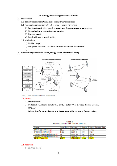
RF Energy harvesting (Possible Outline)1.Introduction1.1C onvert the received RF signals into electricity in various forms1.2Features (in comparison with other kinds of energy harvesting)(1)Far-field: in contrast of inductive coupling and magnetic resonance coupling;(2)Controllable and constant energy transfer;(3)Distance based;(4)Predictable and relatively stable;1.3Motivations:(1)Mobile charge(2)For special scenarios: like sensor network and health-care network(3)…2.Architecture (information source, energy source and receiver node)2.1Sources(1)Static/ dynamic(2)Dedicated / Ambient (Cellular BS/ DMB/ Router/ User Devices/ Radar/ Stellite /FM&AM)(please find the transmit power and frequency for different energy harvest system)2.2Receivers(1)Abstract modela)The application,b)low-power microcontroller: data processingc)low-power RF transceiverd)energy harvester: without power sourceantenna- a range of frequency; impedance matching; voltage multiplier (AC-DC)e)power management module: harvest-use and harvest-store-usef)energy storage or battery(2)Mathematical Model (four types/ SWIPT or seperated)a)Seperated ReceiverReasons: information reception and RF energy harvesting work on very different power sensitivity (e.g., -10 dBm for energy harvesters versus -60 dBm for informationreceivers)??? 为什么敏感度不同就用不同的天线b)Co-located Receiver Architecture: (Time-switching and power splitting, lower powerconsuming circuit)i)Time-switching:Power harvest model:Datarate:ii)Power-splittingPower harvest model:Datarate:c)Integrated Receiver Architecture: (Dynamic Power-Splitting)d)Ideal Type (Unrealistic)The current circuit designs are not yet able to extract RF energy directly from thedecoded information carrier.2.3Channel Model (Propagation Model, refer to the specific scenario)(1)Free space model: one single path(2)Two ray ground model: line-of-sight and a reflection path(3)Probabilistic model: Rayleigh Model3.Open Issues in System Design3.1Device Design(1)Passive Matching Circuit(2)Energy Harvester Circuit(3)Receiver Operation Policy3.2MAC Design(1)Energy Harvest Adaptive CSMA/CA(2)…3.3Multi-User Scheduling(1)Fairness scheduling (maximize the minimum datarate)(2)Throughput maximization scheduling(3)Utilization optimization scheduling3.4Routing Protocol4.Open Application Issues4.1Multiple Antenna System and Beam Forming(1)SWIPT Beamforming Optimization without Secure Communication Requirement (tableV page 15)(2)SWIPT beamforming for Secure Communication (table VI page 18)(3)Energy Beamforming(4)Special Issue: Information Feedback4.2Cooperative Relay Networks(1)Relay operation policy (one source, one relay(one way or two way), one destination)(2)Relay Selection(3)Power Allcoation(4)Precoding(5)Network Coding4.3RF-powered cognitive radio network(1)Dynamic Spectrum Access(2)Mode Selection(3)Channel Selection(4)CRN D2D4.4Wireless Sensor Network(1)…4.5Healthy carelow-power medical devices can achieve real-time work-on-demand power from dedicated RF sources, which further enables a battery-free circuit with reduced size;(可穿戴不用带电池，让电池无线供电)4.6RFID4.7Battery-free devices powered by ambient energy from WiFi [72], [73], GSM [74]–[77] andDTV bands [78]–[83] as well as ambient mobile electronic devices [84]5.Future Directions and Practical Challenges5.1Distributed Energy BeamformingDistributed energy beamforming enables a cluster of distributed energy sources to cooperatively emulate an antenna array by transmitting RF energy simultaneously in the same direction to an intended energy harvester for better diversity gains.5.2Interference ManagementHowever, with RF energy harvesting, harmful interference can be turned into useful energy through a scheduling policy. In this context, how to mitigate interference as well as facilitate energy transfer, which may be conflicting, is the problem to be addressed.5.3Energy TradingThe RF energy market can be established to economically manage this energy resource jointly with radio resource. For example, wireless charging service providers may act as RF energy suppliersto meet the energy demand from network nodes. The wireless energy service providers can decide on pricing and guarantee the quality of charging service.5.4Mobility Factor5.5Network CodingDuring the time slots when relays or senders are not transmitting, they can harvest ambient RF signals. A pioneer study in [234] analyzes the network lifetime gain for a two-way relay network with network coding.5.6Impact on Health5.7Practical Challenge(1)Short transfer distanceHowever, as shown in [35], to realize 5.5u W energy transfer rate with a 4W power (FCUPPER BOUND) source, only the distance of 15 meters is possible.(2)Harvesting rateNeed high gain antenna(3)Circuit design for impedance matching(4)The RF-to-DC conversion efficiency(5)Must be small size, (but only uW/cm^2) how to be small size?(6)Therefore, the RF energy source must be optimally placed to support multiple receivers tobe charged.(7)SWIPT is not suitable when a receiver located at a distance away from an RF transmittermay be able only to decode information and fail to extract energy from the RF signals.(8)Hence, power consumption is always a serious concern in RF-powered devices, whichmay require the re-design of existing schemes and algorithms for conventional networks.(with low computational complexity).。

DOI: 10.12086/oee.2021.200319基于石墨烯超表面的效率可调太赫兹聚焦透镜王俊瑶，樊俊鹏，舒 好，刘 畅，程用志*武汉科技大学信息科学与工程学院，湖北 武汉 430081摘要：本文提出了一种基于石墨烯超表面的效率可调太赫兹聚焦透镜。

该超表面单元结构由两层对称的圆形镂空石墨烯和中间介质层组成，其中镂空圆形中间由长方形石墨烯片连接。

该结构可实现偏振转换，入射到超表面的圆偏振波将以其正交的形式出射，如左旋圆到右旋圆偏振转换。

利用几何相位原理，通过旋转长方形条的方向，透射波会携带额外的附加相位并能满足2π范围内覆盖。

合适地排列石墨烯超表面的单元结构，以实现太赫兹聚焦透镜。

仿真结果表明：通过改变石墨烯的费米能级，可以对超表面圆偏振转换幅度进行调节，进而超透镜的聚焦效率也可以动态调节。

因此，这种基于石墨烯超表面的效率可调聚焦透镜不用改变单元结构的尺寸，只需通过改变费米能级便可实现，可以广泛地应用到能量收集、成像等太赫兹应用领域。

关键词：超表面；聚焦透镜；石墨烯；太赫兹中图分类号：TH74；TQ127.11 文献标志码：A王俊瑶，樊俊鹏，舒好，等. 基于石墨烯超表面的效率可调太赫兹聚焦透镜[J]. 光电工程，2021，48(4): 200319Wang J Y , Fan J P , Shu H, et al. Efficiency-tunable terahertz focusing lens based on graphene metasurface[J]. Opto-Electron Eng , 2021, 48(4): 200319Efficiency-tunable terahertz focusing lens based on graphene metasurfaceWang Junyao, Fan Junpeng, Shu Hao, Liu Chang, Cheng Yongzhi *School of Information Science and Engineering, Wuhan University of Science and Technology, Wuhan, Hubei 430081, China Abstract: This paper proposes an efficiency-tunable terahertz focusing lens based on the graphene metasurface. The unit cell is composed of two symmetrical circular graphene hollows and an intermediate dielectric layer, wherein the hollow circular middle is connected by a rectangular graphene sheet. This structure can realize polarization conversion, for example, when an incidence with left-hand circular polarization emitted on the metasurface the po-larization of the transmitted light is right-hand circular polarization. According to the principle of geometric phase, by rotating the direction of the rectangular bar, the transmitted wave will carry an additional phase and can cover the range of 2π. An THz focusing lens can be realized by properly arranging the unit structure of the graphene metasurface. The simulation results show that the conversion amplitude of circular polarized light can be adjusted by changing the Fermi level of graphene, and the focusing efficiency of the metalens can also be dynamically adjusted.LCPRCP(cross-polarization)xy zV g——————————————————收稿日期：2020-08-27； 收到修改稿日期：2020-10-26基金项目：湖北省教育厅科技研究计划重点项目(D2*******)；武汉科技大学研究生创新基金项目(JCX201959)；大学生创新基金项目资助课题(20ZA083)作者简介：王俊瑶(2000-)，女，主要从事电子科学与技术专业。

仿生鱼鳍单元设计及运动仿真分析何建慧;章永华【摘要】Based on motor-cam-slider-crank mechanism,a biomimetic fish fin unit was developed.Then,the kinematics of biomimetic fish fin unit was analyzed,the relationship between cam and fin ray was also established.In combination with Adams simulation software,the change of angular displacement,angular velocity and angle acceleration of fin ray was presented under different cam angular velocities of π/6 rad·s-1 and 2π/3 rad·s-1.The results indicate that:the curves of angular displacement,angular velocity and angle acceleration with time present the same undulating rule with equal frequency.However,the ray angular acceleration time curve presents small asymmetry relative to the zero line.Moreover,the frequency and the amplitude of angular displacement,angular velocity and angle acceleration increase with the increase of motor rotation velocity.This motion characteristics coincide with the motion law of biological fins.The development of current biomimetic fish fin unit provides a reference for the further research on bio-propulsor.%利用电机-凸轮-滑块-曲柄机构,设计了一款仿生鱼鳍单元.对仿生鱼鳍单元的运动学进行分析,建立了凸轮运动参数与鳍条运动参数之间的关系.结合Adams仿真软件,分析凸轮角速度分别为π/6和2π/3 rad·s-1时鳍条运动角位移、角速度和角加速度随时间的变化.结果显示:鳍条角位移、角速度和角加速度曲线均呈现等频率波动规律,但鳍条角加速度时间曲线相对零位呈现小幅度的不对称性;随着电机转速增加,鳍条角位移、角速度和角加速度的变化频率增大,幅值也随之增大.上述运动特征与生物鱼鳍的运动规律相符,该仿生鱼鳍单元结构设计为进一步研制仿生鳍推进器提供参考.【期刊名称】《系统仿真技术》【年(卷),期】2017(013)002【总页数】5页(P170-174)【关键词】仿生鱼鳍;鳍条;凸轮;曲柄-滑块机构【作者】何建慧;章永华【作者单位】台州职业技术学院机电工程学院,浙江台州 318000;台州职业技术学院机电工程学院,浙江台州 318000【正文语种】中文【中图分类】TP242.6鱼类因非凡的运动能力使其能够在复杂的水下环境中生存[1],这一点引起了研究人员广泛的关注,并于近二十年内开发了大量的仿生机器鱼推进器。

a r X i v :h e p -t h /0609116v 1 17 S e p 2006Casimir energy of two plates inside a cylinder.∗Valery N.Marachevsky †V.A.Fock Institute of Physics,St.Petersburg State University,198504St.Petersburg,RussiaFebruary 2,2008AbstractThe new exact formulas for the attractive Casimir force acting on each of the two perfectly conducting plates moving freely inside an infinite perfectly conducting cylinder with the same cross section are derived at zero and finite temperatures by making use of zeta function technique.The short and long distance behaviour of the plates’free energy is investigated.1IntroductionRecently a new geometry in the Casimir effect[1],a piston geometry,has been introduced in a 2D Dirichlet model [2].Generally the piston is located in a semi-infinite cylinder closed at its head.The piston is perpendicular to the walls of the cylinder and can move freely inside it.The cross sections of the piston and cylinder coincide.Physically this means that the approximation is valid when the distance between the piston and the walls of a cylinder is small in comparison with the piston size.In paper [3]a perfectly conducting square piston at zero temperature was investigated in 3D model in the electromagnetic and scalar case.The exact formula (Eq.(6)in [3])for the force on a piston was written in the electromagnetic case.Also the limit of short distances was found for arbitrary cross sections (Eq.(7)in [3]).This result was generalized in [4].In paper [4]the exact formula for the free energy of two perfectly conducting plates ofan arbitrary cross section inside the waveguide(or infinite cylinder)with the same cross section was written(Eq.(118)in[4]or(30)here).In the zero temperature case and square cross section of the waveguide our general result for the force(35)coincides with Eq.(6)in[3].It is interesting that our result resembles the result for the interquark potential in a rigid string model[5].A dilute circular piston and cylinder were studied perturbatively in[6]. In this case the force on two plates inside a waveguide and the force in a piston geometry differ essentially.The force in a piston geometry can even change sign in this approximation for thin enough walls of the material. Other examples of repulsive pistons were presented in[7].In Sec.2we derive the new exact result(30)for the free energy of two parallel plates inside an infinite cylinder by making use of the zeta function technique[8,9].We consider a perfectly conducting case,the plates move freely inside the cylinder with the same cross section,which is arbitrary. The plates are perpendicular to the walls of the cylinder.In Sec.3we apply the heat kernel technique[10,11,4]to derive the leading short distance behaviour of the free energy.In the short distance limit we prove that there are no temperature corrections to the leading terms obtained in[3](Eq.(7)in [3]).The long distance limit result(40)(the high temperature limit result) is new.We take =c=1.2DerivationOur aim is to calculate the Casimir energy of interaction and the force be-tween the two parallel plates of an arbitrary cross section inside an infinite cylinder of the same cross section(the plates are perpendicular to the walls of the cylinder).T E and T M eigenfrequencies of the perfectly conducting cylindrical res-onator with an arbitrary cross section can be written as follows.For T E modes(E z=0)inside the perfectly conducting cylindrical resonator of the length a with an arbitrary cross section the magneticfield B z(x,y,z)and2eigenfrequenciesωT E are determined by:B z(x,y,z)=+∞i=1,n=1B in sin πnz∂n ∂M=0(3)ω2T E= πna f k(x,y),(5)∆(2)f k(x,y)=−λ2kD f k(x,y)(6) f k(x,y)|∂M=0(7)ω2T M= πn2 ω1−s T E+ ω1−s T M s=0,(9)where the sum has to be calculated for large positive values of s and after that an analytical continuation to the value s=0is performed.Alternatively one can define the Casimir energy via a zero temperature one loop effective action W(T1is a time interval here):W=−ET1(10) E=−ζ′(0)(11)ζ(s)=12) +∞0dt t s2πexp−t aIn every Casimir sum it is convenient to write:+∞n=1exp(−tn2)=12=1π −1√x (14)and the value of the integral+∞dt tα−1exp −p t−q p αpq)(15) for nonzero values of n to rewrite the Neumann zeta functionζN(s)(arising from TE modes)in the form:ζN(s)= λiN +∞−∞dpπΓ (s−1)/2 λ2iN+p2πa 2K s−1λ2iN+p2 −− λiN√4aΓ(s/2) aλiN2π1λ2iN+p2) ++a2π λ2iN+p21−s4λiNλ1−siN s=0.(17)Here we used K−1/2(x)=2π1λ2kD+p2) ++a2π λ2kD+p21−s4λkDλ1−skD s=0.(18)4The electromagnetic Casimir energy of a perfectly conducting resonator of the length a and an arbitrary cross section is given by the sum of (17)and (18):E = λiN +∞−∞dp2ln 1−exp(−2a2π1λ2kD +p 2) +(20)+a 2π λ2iN+p 21−s 2 λkD+∞−∞dp 2s =0+(22)+14 λiNλ1−s iNs =0.(23)The termsE waveguide =12πλ2iN +p21−s2 λkD+∞−∞dp2s =0(25)yield the electromagnetic Casimir energy for a unit length of a perfectlyconducting infinite cylinder with the same cross section as the resonator under consideration.For the experimental check of the Casimir energy for the rectangular cavity one should measure the force somehow.We think about the following possibility:one should insert two parallel perfectly conducting plates inside an infinite perfectly conducting cylinder and measure the force acting on one of the plates as it is being moved through the cylinder.The distance between the inserted plates is a .To calculate the force on each plate the following gedanken experiment is useful.Imagine that 4parallel plates are inserted inside an infinite cylinder and then 2exterior plates are moved to spatial infinity.This situation is exactly equivalent to 3perfectly conducting cavities touching each other.From the energy of this system one has to subtract the Casimir energy of an infinite cylinder,only then do we obtain the energy of interaction between the interior parallel plates,the one that can be measured in the proposed5experiment.Doing so we obtain the attractive force on each interior plate inside the cylinder:F(a)=−∂E arb(a)2ln(1−exp(−2aωwave)),(27)the sum here is over all T E and T M eigenfrequenciesωwave for the cylinder with an arbitrary cross section and an infinite length.Thus it can be said that the exchange of photons with the eigenfrequencies of an infinite cylin-der between the inserted plates always yields the attractive force between the plates.For rectangular boxes it was generally believed[12,13]that the repulsive contribution to the force acting on two parallel opposite sides of a single box(separated by a distance a)and resulting here from(21-22)could be measured in experiment.However,it is not possible to use the expression (19-23)directly to calculate the force since it includes the self-energy Casimir parts(21-22)of the other sides of the resonator.Nevertheless the expression (19-23)can be used to derive a measurable force(26)between the freely moving parallel plates inserted inside an infinite cylinder of the same cross section as the plates.To get the free energy F arb(a,β)for bosons at nonzero temperatures(β= 1/T)one has to make the substitutions:p→p m=2πm2π→1β λkD +∞m=−∞1λ2kD+p2m) ++12ln 1−exp(−2aplate inside the cylinder):∆(2)f k(x,y)=−λ2kD f k(x,y)(31)f k(x,y)|∂M=0,(32)∆(2)g i(x,y)=−λ2iN g i(x,y)(33)∂g i(x,y)∂a=−1exp(2aωT D )−1−1exp(2aωT N)−1.(35)HereωT D= p2m+λ2iN.3Asymptotic casesIt is convenient to apply the technique of the heat kernel to obtain the short distance behaviour of the free energy(30).It can be done by noting that if the heat kernel expansionλi e−tλ2i∼t→0+∞ k=0t−n+ktλi∼t→0n−1 k=02Γ(n−k)2c k(37)by making use of the analytical structure of the zeta function.The strategy is the following:one expands the logarithms in the formula(30)in series and then applies the expansion(37)to each term.For a≪β/(4π)one obtains from(30)and(37)the leading terms for the free energy:F arb(a,β)|a≪β/(4π)=−ζR(4)a3−ζR(2)whereχ=i1αi−αi12πγjL aa (γj )dγj .(39)Here αi is the interior angle of each sharp corner and L aa (γj )is the curvature of each smooth section described by the curve γj .The force calculated from (38)coincides with F C in [3],(Eq.7).In the opposite long distance limit a ≫β/(4π)one has to keep only m =0term in (30).Thus the free energy of the plates inside a cylinder in this limit (the high temperature limit)is equal to:F arb (a,β)|a ≫β/(4π)=12βλiNln 1−exp(−2aλiN )(40)This result is new.One can check that the limit a →0in (40)immediately yields the high temperature result for two parallel perfectly conducting plates separated by a distance a .One expands logarithms in series and uses (37)and c 0D =c 0N =S/(4π)in two dimensions (n =2)to obtain:F arb (a,β)|a ≫β/(4π),a →0==−λkD1na →0− λiN1na →0==+∞ n =1−1n1βa 2S[2]R.M.Cavalcanti,Phys.Rev.D72,065015(2004)[arXiv:quant-ph/0310184].[3]M.P.Hertzberg,R.L.Jaffe,M.Kardar and A.Scardicchio,Phys.Rev.Lett.95,250402(2005)[arXiv:quant-ph/0509071].[4]V.N.Marachevsky,One loop boundary effects:techniques and applica-tions[arXiv:hep-th/0512221].[5]V.V.Nesterenko and I.G.Pirozhenko,J.Math.Phys.38,6265(1997)[arXiv:hep-th/9703097].[6]G.Barton,Phys.Rev.D73,065018(2006).[7]S.A.Fulling and J.H.Wilson,Repulsive Casimir Pistons[arXiv:quant-ph/0608122].[8]E.M.Santangelo,Theor.Math.Phys.131,527(2002);Teor.Mat.Fiz.131,98(2002)[arXiv:hep-th/0104025].[9]E.Elizalde,S.D.Odintsov,A.Romeo,A.Bytsenko and S.Zerbini,”Zetaregularization with applications”,World Sci.,Singapore,1994.[10]D.V.Vassilevich,Phys.Rept.388,279(2003)[arXiv:hep-th/0306138].[11]P.B.Gilkey,”Invariance theory,the heat equation,and the Atiyah-Singer index theorem”,CRC Press,1994.[12]W.Lukosz,Physica(Amsterdam)56,109(1971).[13]M.Bordag,U.Mohideen,V.M.Mostepanenko,Phys.Rept.353,1(2001)[arXiv:quant-ph/0106045].[14]I.Brevik,S.A.Ellingsen and ton,Thermal corrections to theCasimir effect[arXiv:quant-ph/0605005].[15]F.Sauer,PhD Thesis Gottingen,1962.[16]E.M.Lifshitz,Zh.Eksp.Teor.Fiz.29,94(1956)[Soviet Phys.JETP2,73];I.D.Dzyaloshinskii,E.M.Lifshitz and L.P.Pitaevskii,Usp.Fiz.Nauk 73,381(1961)[Soviet p.4,153].9。

去参观农场英语作文优秀9篇（经典版）编制人：__________________审核人：__________________审批人：__________________编制单位：__________________编制时间：____年____月____日序言下载提示：该文档是本店铺精心编制而成的，希望大家下载后，能够帮助大家解决实际问题。

文档下载后可定制修改，请根据实际需要进行调整和使用，谢谢!并且，本店铺为大家提供各种类型的经典范文，如工作资料、求职资料、报告大全、方案大全、合同协议、条据文书、教学资料、教案设计、作文大全、其他范文等等，想了解不同范文格式和写法，敬请关注!Download tips: This document is carefully compiled by this editor.I hope that after you download it, it can help you solve practical problems. The document can be customized and modified after downloading, please adjust and use it according to actual needs, thank you!In addition, this shop provides you with various types of classic model essays, such as work materials, job search materials, report encyclopedia, scheme encyclopedia, contract agreements, documents, teaching materials, teaching plan design, composition encyclopedia, other model essays, etc. if you want to understand different model essay formats and writing methods, please pay attention!去参观农场英语作文优秀9篇在生活、工作和学习中，大家都写过作文吧，写作文可以锻炼我们的独处习惯，让自己的心静下来，思考自己未来的'方向。

E nergy Procedia 48 ( 2014 )524 – 534Available online at ScienceDirect1876-6102 © 2014 The Authors. Published by Elsevier Ltd.Selection and peer review by the scienti fi c conference committee of SHC 2013 under responsibility of PSE AGdoi: 10.1016/j.egypro.2014.02.062D aniel Carbonell et al. /E nergy Procedia 48 ( 2014 )524 – 534 5251.IntroductionThe need for reducing fossil fuel dependency is pushing the combination of different technologies in order to increase the renewable energy usage at worldwide level. Among them, the combination of solar thermal and heat pumps is an attractive option for heating and domestic hot water preparation with a high share of local renewable energy use. Nevertheless, when combining the solar thermal technology with heat pumps several problems may occur that need to be avoided. The combination leads to a more complex system where poor design can lead to a significantly lower performance than expected. Control strategies and system hydraulics, in particular the combination of heat pumps with combi-storage tanks, can strongly influence the system performance and have been identified as a possible source of poor performance [1]. System analyses are of importance to provide recommendations for system design and standard solutions, which are key aspects to allow these combined technologies to spread worldwide.In this work both parallel and series combined solar and heat pump systems are considered. Parallel systems have the advantage of being less complex than the series ones in terms of hydraulic connections and system control and therefore, parallel systems may be more robust and reliable. Nevertheless, some series systems based on solar assisted heat pumps with brine or ice storages are also of interest. A system with an ice storage can be an attractive alternative to a ground source heat pump when, for example, regulations forbid to drill a borehole. These systems can also be seen as an alternative to air source systems when efficiency or noise problems are of importance. Therefore, one type of these systems based on a large ice storage with immersed flat plate heat exchangers that can be de-iced is also studied in this work. Moreover, a reference case without solar is used to determine the potential benefits of using solar collectors compared to a system with a heat pump alone. In order to have the whole picture of the benefits of adding solar thermal to a heat pump, it is necessary to simulate the systems under several climates. This is out of the scope of the present work and has been presented in a separate paper [2].Reference conditions defined in the framework of the International Energy Agency (IEA), Solar Heating and Cooling programme (SHC Task 44) and Heat Pump programme (HPP Annex 38) “Solar and Heat Pumps”[3], known under the combined name Task44/Annex38 (T44/A38) are employed in order to analyze different systems combining solar and heat pumps under the same boundary conditions. Results are presented for three buildings and the typical Central European moderate climate of Strasbourg.The need for reliability in the results when modeling different systems is a key aspect and since validation with experimental data for all systems is very time consuming, two simulation environments have been employed: TRNSYS-17 () and Polysun-6® (http://www.polysun.ch). The simulation with both tools is not only useful to find inconsistencies in each simulation, but also it forces to analyze possible sources of difference and therefore helping to understand the different hypothesis used that may cause the discrepancies. Furthermore, it is also important to validate and analyze modeling tools used for planners and engineers since most of the people who will install these systems will not use TRNSYS, which more widely employed in the research community, and reliable and robust modeling tools are very important for a correct design of these systems.2.MethodologySimulations have been conducted using two simulation platforms: TRNSYS-17 (TN) and Polysun-6® (PS). The present TN simulations are carried out using the state of the art of the component models that have been validated separately in different works. The system configuration in TN is being extensively used and improved by several research institutes, most currently in the framework of the ongoing EU-FP7 project “MacSheep” (http://macsheep.spf.ch/).The space heating (SH) loads have been introduced as a heat sink element in PS. The heating loads were previously calculated with TN building model Type-56. The domestic hot water (DHW) tapping profile is obtained from T44/A38 [4], the DHW set temperature is 45°C and the cold water temperature is 10o C.Results have been obtained for three buildings SFH15, SFH45 and SFH100 of T44/A38 (see [4,5] for details) in Strasbourg. The three buildings represent a low (SFH15), medium (SFH45) and high (SFH100) building energy526D aniel Carbonell et al. / E nergy Procedia 48 ( 2014 )524 – 534demand (Q d), where SFH stands for Single Family House and the numbers, 15 for example, for the yearly energy demand in kWh/m2 per building heated surface area in the city of Strasbourg. The buildings SFH15 and SFH45 have low temperature heat distribution systems (T flow,max=35°C and T return,max=30°C) and the building SFH100 has a higher temperature heat distribution system (T flow,max=55°C and T return,max=45°C).The combined parallel systems consist of a combi-storage as a connecting component between the heat delivered from the heat pump, the solar thermal heat input, and the useful energy delivered to DHW or SH. The considered parallel systems are a combination of a Solar thermal system with an Air Source Heat Pump (SASHP) and a Solar thermal system with a Ground Source Heat Pump (SGSHP). In the series systems analyzed here, the solar energy can be directed to the combi-storage or to the heat pump, either directly or indirectly through an ice storage.Therefore, strictly speaking, the system concept is based on a combination of parallel and series. For simplifications reasons the concept of this system will be referred to as series. This system is labeled as a combined Solar and Ice storage Source Heat Pump (SISHP). In order to show the possible energy flows within the systems the energy flow chart of T44/A38 introduced by Frank et al. [6] is used in Fig.1 to present the scheme of the parallel SASHP (left) and the series SISHP (right) systems.The combi-storage has separate connections for charging the storage DHW and SH zones by the heat pump. As recommended by Haller et al. [1], the return line from the storage to the heat pump in DHW charging mode is above the zone affected by SH operation, and the position of the sensor used for DHW charging control is well above the space heating zone of the combi-storage. For PS simulations it is important to have the return line from the storage to the heat pump in the DHW section at least one layer above the inlet of the heat pump to the SH section of the combi-storage. Otherwise some numerical mixing occurs due to the low and fixed number of control volumes (n cv=12) included in the PS storage tank.Fig. 1 Energy flow chart visualization scheme [4] for parallel SASHP (left) and SISHP (right).The "heat pump only" reference system is defined similar as the combined system (same components) but without the solar part. Since systems using only heat pumps will most likely be installed without a combi-storage, the reference system is designed with two storage tanks; one 300 l tank for DHW and another 200 l tank for SH.Polysun-6® has a very versatile user defined control function that allows implementing the control used in TN more easily. Therefore the same control strategies were implemented in the two simulation platforms.All results presented using PS have been obtained from hourly results data with a validated post-processing tool.The post-processing has been used to recalculate some values as for example the electricity consumption of circulating pumps or control units for the heat pump and the solar thermal system. Moreover, user defined performance indicators, as the ones defined in section 2.1, were calculated from hourly values. For the electricity consumption of the control unit a constant value of 3 W during all the year has been assumed. Energy balances for every loop are also calculated to ensure proper use of values when computing the performance indicators. The same post-processing is also employed for TN simulations in order to avoid differences in the post-processing task.D aniel Carbonell et al. /E nergy Procedia 48 ( 2014 ) 524 – 534 527Performance Factor calculated as described in [8] by: T el SH DHW T el SH SHP Q Q dt P dt Q Q ,,)( is the time step in [s];Q is the heat load power in [W] and is the yearly heat load energy and P and SH stand for solar and heat pump, domestic hot water electricity consumption is calculated as:el cu el hp el pu el P P P P , where the subscripts pu , , cu respectively. The symbol "+" in the SHP+ from Eq.1 refers to the consideration of the heat distribution circulating pump in the electricity consumption. Therefore the term The seasonal performance factor of the heat pump alone is defined as:dt P dt Q hp con HP is the heat delivered by the condenser of the heat pump. In order to compare results from one simulationof a particular system (SHP+) to the reference system (ref) the relative increase of SPF is used:SHP SHP SPF SPF SPF SPF Another figure for the comparison between systems is the fractional solar electricity savings defined as: SHPsave P f ((1 The absolute electricity savings are calculated as follows:SHP el P P ((528 D aniel Carbonell et al. / E nergy Procedia 48 ( 2014 ) 524 – 534calculated in PS because including a new system is much easier with this simulation tool. Despite of the fact that TN and PS can predict different system performance in absolute terms, the relative difference between two simulations, i.e. combined solar and heat pump and “heat pump alone” systems, within the same platform are not expected to be very different between TN and PS. Therefore the study with only one simulation platform should be enough in this case.3.1. Analysis of parallel systems. Comparison between TRNSYS and Polysun-6®A comparison task between TN and PS simulations for combined SASHP and SGSHP parallel systems has been undertaken to obtain insights into the capabilities and limitations of each modeling platform. Numerical results for all buildings and simulation environments are presented in Table 1. All this simulations are obtained using 15 m 2 of collector area (C A ). The first two columns of the central section of Table 1 are used to present the amount of energy the heat pump provides to DHW, DHW HP Q , and to SH, SH HP Q ,. These terms are particularly important for the heat pump performance and mostly depend on control settings and positions of the inlet and outlet connections between the heat pump and the storage, as well as on the stratification capabilities of the storage [1]. For SFH15 and SFH45 the DHW section of the combi-storage is at higher temperatures compared to the SH section. However, this is not the case for SFH100 because of the high temperature (T flow =55°C) of the distribution system (see section 2). For this reason, providing more energy at DHW level decrease the heat pump performance for SFH15 and SFH45, but it does not for SFH100. These two terms are quite similar between TN and PS for SFH15 and SFH45 for both SASHP and SGSHP, but not for SFH100.In the right section of Table 1 relative differences between the two simulation tools are shown for the SPF of the heat pump and of the system performance as described in section 2.1. In this case TN simulations are considered to be the reference. PS tends to predict lower values of HP SPF for both SASHP and SGSHP systems (see the sign of the HP SPF ) with relative differences always below 3% for SASHP and below 13.5% for SGSHP systems. The HP SPF of SASHP systems is quite similar between TN and PS. However for SGSHP systems, the discrepancies of heat pump alone performance are more significant. The main reason for this is thought to be the lower source (borehole) temperature predicted by PS when compared to TN. This is surprising since both platforms use the same ground heat exchanger model (EWS [10]). However, PS is using a newer version of the EWS model, while TN-EWS model is quite old. Nevertheless it would be surprising if the modifications of the newer version are the cause of such differences.The differences in system performance SHP SPF are below 4.6% for SASHP (quite good result) and below 13.5% for SGSHP systems.Table 1. Results of SASHP and SGSHP for different building loads as simulation software: TRNYS-17 (TN) and Polysun-6® (PS).System Platformc A Building DHW HP Q , SH HP Q ,d Q T el P , HP SPF SHP SPF HP SPF SHP SPF[m 2] SFH [MWh] [MWh] [MWh] [MWh] [−] [−] [%] [%] S ASHPTN 15 15 0.57 2.14 4.55 1.15 2.87 3.83 - - SASHPPS 15 15 0.55 2.02 4.65 1.05 2.80 4.00 -2.38 4.5 SASHPTN 15 45 0.75 5.58 8.55 2.26 3.14 3.69 - - SASHPPS 15 45 0.63 5.37 8.39 2.10 3.07 3.56 -2.22 -3.68 SASHPTN 15 100 0.53 13.00 16.12 5.93 2.43 2.69 - - SASHPPS 15 100 0.00 13.77 15.84 5.82 2.50 2.65 2.76 -1.44 SGSHPTN 15 15 0.57 2.15 4.55 0.73 4.90 5.90 - - SGSHPPS 15 15 0.60 2.09 4.64 0.72 4.44 5.73 -9.36 -2.97 SGSHPTN 15 45 0.73 5.60 8.55 1.41 5.39 5.83 - - SGSHPPS 15 45 0.72 5.51 8.45 1.37 5.04 5.06 -6.44 -13.31 SGSHPTN 15 100 0.90 12.65 16.12 3.60 4.26 4.40 - - SGSHPPS 15 100 0.00 13.90 15.81 3.96 3.69 3.85 -13.29 -12.34D aniel Carbonell et al. /E nergy Procedia 48 ( 2014 ) 524 – 534 529The SHP SPF depends on the HP SPF and T el P ,. Therefore the difference in one term may be compensated by the other, see for example that SHP SPF for SGSHP and SHF15 is lower than the HP SPF for the same case.In order to understand the possible source of differences, main yearly heat flows are presented for SASHP in Fig. 1(a) and for SGSHP in Fig. 1(b) for all building load demands. In Fig. 1 it can be seen that the solar yield is very similar between both simulation tools with a larger difference for the SFH100 building. SH demands are almost the same because a heat sink has been used in PS in order to meet reference system heating loads (see section 2). Storage losses are also in the same range of magnitude between both platforms. Piping losses in these simulations are lower in PS. Losses due to frosting and auxiliary heating of the heat pump are accounted in PS. Nevertheless, cycling and thermal losses are neglected in PS. This may be the reason the evaporator heat reported for TN is much higher than for PS. Consequently, the operating hours of the heat pump and of circulation pumps in the heat pump loop are also higher in TN. These heat pump losses are, however, more important in a series system where the source of the heat pump is the collector field (more collector area will be needed if heat pump losses would be accounted for in PS). In the case of SGSHP the higher evaporation needs are obtained from the ground so this will imply higher extraction from the ground. Heat pump losses are lower for GSHP systems than for ASHP as it can be seen in comparing this term from Fig. 1(a) and Fig. 1(b).Fig. 2. Yearly energy balances comparison between TN (left bar) and PS (right bar) simulations for (a) SASGP and (b) SGSGP systems. The electricity consumption distribution terms for SASHP SFH15 are shown in Fig.3 (left) for TN. Most of the energy consumed is from the heat pump compressor. In this case the backup heating is included as a heating rod in the heat pump unit to provide extra energy for DHW when needed. The ventilator is also part of the heat pump unit. Circulating pumps are in second position of importance. The controller units consumption are independent of the heating demand, therefore it is a relevant factor for SFH15 but not very important for SFH100. The controller unit and circulating pumps consumption losses share on total electricity demand decrease for higher energy demand buildings.In Fig. 3(b) it can be observed that PS predicts lower values for the electricity consumption of pumps. This is the reason, besides the high share of the circulating pumps respect to the total, of having higher discrepancies for SFH15 in SASHP. In particular, the number of operating hours of the collector pump is constantly much lower in PS than in TN. The authors found that the outlet temperature of the collector in PS shows short term oscillations that lead to on/off cycling of the solar pump. The hourly averaged values for outlet temperature and power are similar to TN,530 D aniel Carbonell et al. / E nergy Procedia 48 ( 2014 ) 524 – 534but not the running time of the solar pump. In SASHP, as commented before, the number of operating hours of theheat pump is higher because of the neglected losses of the heat pump, this also affects the circulation pumps of theheat pump loop. In SGSHP the circulation pumps have a much closer value in terms of operating hours between both simulation tools because heat pump losses are less important. Nevertheless, the pumps consumption depends on nominal flow conditions and these are different for both simulation tools because of different manufacturers heat pump models used. Using mass flow rates that deviate substantially from the nominal conditions produced unrealistic results in PS and it is therefore not recommended.Fig. 3. Yearly electricity consumption distribution using TN for SASHP-SFH15 (left). Comparison between TN and PS for SFH45 and bothSASHP and SGSHP systems (right).3.2. Comparison of parallel systems against reference “heat pump alone” systemsThe comparisons between coupled solar and heat pump systems against a reference system using only a heat pump, labeled as “heat pump alone” systems has been performed using PS.Simulation results for the solar thermal and heat pump combinations SGSHP and SASHP, as well as for the “heat pump alone” systems GSHP and ASHP are presented in Table 2. In the right section of Table 2 the change of performance indicators (see section 2.1) with respect to the reference "heat pump only" system are shown.Table 2. Results of (S)ASHP and (S)GSHP for different building loads.System Building DHW HP Q , SH HP Q , d Q T el P ,HP SPF SHP SPF HP SPF SHP SPF el save f , el save P , SFH [MWh] [MWh][−] [−] [%] [%] [%] [MWh] ASHP 15 2.57 2.66 4.64 1.783.23 2.61 - - - - SASHP 15 0.55 2.024.65 1.052.80 4.00 -13.34 53.13 40.86 0.73 ASHP 45 2.61 6.19 8.14 2.793.37 2.92 - - - - SASHP 45 0.63 5.37 8.39 2.103.07 3.56 -8.81 21.89 24.67 0.69 ASHP 100 2.61 14.21 15.956.932.58 2.30 - - - - SASHP 100 0.00 13.77 15.84 5.822.50 2.65 -3.04 15.18 16.05 1.11 GSHP 15 2.59 2.684.68 1.334.35 3.52 - - - - SGSHP 15 0.60 2.10 4.65 0.724.445.73 0.21 62.90 45.88 0.61 GSHP 45 2.606.55 8.55 2.004.91 4.27 - - - - SGSHP 45 0.725.51 8.45 1.375.04 5.06 2.00 18.41 31.43 0.63 GSHP 100 2.60 14.06 15.86 4.603.80 3.45 - - - - SGSHP 100 0.00 13.93 15.82 3.963.69 3.85 -2.87 11.70 13.84 0.64D aniel Carbonell et al. /E nergy Procedia 48 ( 2014 ) 524 – 534 531For all simulations, the improvement in terms of fractional electricity savings el save f , is significant when the solar thermal system is added and it tends to be higher for low energy buildings and for SGSHP compared to SASHP systems.For the ASHP (see upper part of Table 2), the heat pump performance (HP SPF ) decreases when the solar thermal system is added being a more important effect for low energy demand buildings. Despite of this, the SHP SPF increases because the solar thermal system has a much higher ratio of heat delivered to electricity consumed compared to the heat pump. As observed in [2], when the solar thermal system is added to an air source “heat pump alone system”, two opposite effects in terms of performance can be observed in the behavior of the heat pump. On one hand the heat pump performance (HP SPF ) decreases because the solar thermal system covers part or all of the loads at times when the ambient temperature is moderately high, i.e. spring and summer periods, where also the performance of the air source heat pump is best. On the other hand, the performance of the heat pump alone (HP SPF ) slightly increases when the solar system is added because the solar thermal collectors cover some of the DHW loads at high temperature and therefore the heat pump works less time at high sink temperatures (see differences of DHW HP Q , between combined and “heat pump alone” systems). The share of DHW on the total heat demand also plays a role here. On a yearly basis the decrease of the heat pump alone performance for not working at the best periods is usually dominant and therefore the combined system SASHP, has a lower HP SPF compared to the ASHP.For the GSHP system (see bottom part of Table 2), the performance of the heat pump alone (HP SPF ) increases when the solar system is added for SFH15 and SFH45 because, as commented above, the heat pump works less time at high sink temperatures. However, for SFH100 this effect is not observed because of the high flow temperature of the heating distribution system and the lower share of DHW on the total heat demand.The potential benefit in terms of el save f , is higher for SGSHP compared to SASHP systems. However the absolute electricity savings depend on the combination of the fractional savings el save f ,and total electricity consumption of the reference “heat pump only” system. Since the latter is quite higher for ASHP than for GSHP, the absolute electricity savings of SASHP is higher than for SGSHP systems as can be observed in Table 2. In a study conducted in several cities around Europe [2] it has been shown that SASHP in general achieve higher el save P ,compared to SGSHP systems.3.3. Analysis of a SISHP systemIn this section, an ice storage system based on immersed flat plate heat exchangers that can be de-iced is presented and simulated. The system concept has been explained by Philippen et al. [11] and the ice storage model description and validation has been provided by Carbonell et al. [9]. A short explanation of the ice system concept is provided hereafter.When the heat pump extracts heat from the ice storage the growing ice layers on the heat exchanger decrease the overall heat transfer coefficient from the ice forming layer to the brine in the heat exchanger. As a result lower brine temperatures and heat pump performance are obtained. A strategy to prevent the effect of a decreasing overall heat transfer coefficient is to remove the ice layers periodically. The heat exchanger is de-iced before reaching too low brine temperatures by melting a small amount of ice that is in contact with the heat exchanger when the heat pump is switched off. When the melted ice thickness is large enough, the ice layers separate from the heat exchangers and due to buoyancy forces they are accumulated at the water surface of the ice storage.Since ice storages can be considered as an alternative to ground source heat pump systems, the SGSHP system is used here a as reference. Systems based on large ice storages as the ones proposed here would not make sense for low energy buildings due to cost and space reasons, therefore only SFH45 and SFH100 are simulated in this case. As an illustrative example of the behavior of the ice storage tank, a monthly energy balance plot (left axis) has been presented in Fig. 4 for SISHP-I20A20 (see Table 3 for nomenclature) case and building SFH45. The terms presented in the legend from top to bottom are: the heat input from the collector field (heat Q ), the gains (positive y-axis) and losses (negative y-axis) due to ice storage and ground exchange (loss gain Q ,), the heat released gains (positive y-axis) and accumulated (negative y-axis) in the ice storage in form of sensible heat (acum release Q ,), the532D aniel Carbonell et al. / E nergy Procedia 48 ( 2014 )524 – 534energy of ice formation (formiceQ,), the energy extracted from the heat pump (coolQ), the energy used to melt the icein the heat exchangers (hxmeltQ,), the energy used to melt de floating ice at the surface of the ice storage ( floatingmeltQ,).Ice is formed from December to February when the solar energy is not able to balance the heat extraction of the heat pump and the ice storage is still not charged of sensible energy. Notice for example that in October and November, no ice is formed because the ice storage is full of sensible energy from the summer and therefore theheat released term of the ice storage is very high (see acumreleaseQ,term on the positive y-axis of Fig. 4).Fig. 4. Monthly and yearly energy balances of and ice storage for the SISHP-I20A25 and building SFH45 using TN.The solar collector input (heatQ) increase from November to February, where the maximum solar energy is used by the ice storage, and afterwards the solar energy decreases until October where the minimum solar energy input is found. The time of maximum usage of solar energy correspond the month of maximum ice melted. From January to March the solar input correlates well with the floating ice melting. In summer the ice storage is almost charged of sensible heat (average temperature in August is around 65°C), and during these months most of the solar energy is used for balancing the losses to the ground. From November to March the storage gains energy from the ground, and from April to October the storage losses energy to the ground.Table 3. Results of several SISHP systems compared against SGSHP reference system for different building loads.System BuildingiceV c A uncA d Q T el P,HPSPF SHPSPF HPSPF SHPSPFSFH [m2] [m2] [m2] MWh] [MWh] [−][−][%] [%]SGSHP 45 - 15 0 8.55 1.41 5.39 5.83 - -SISHP-I20A20 45 20 20 5 8.52 1.41 5.42 5.53 0.64 -8.31SISHP-I20A30 45 20 30 5 8.52 1.26 5.61 5.90 4.12 1.13SISHP-I25A15 45 25 15 5 8.52 1.52 5.35 5.01 -0.82 -14.17SGSHP 100 - 15 0 16.12 3.60 4.26 4.40 - -SISHP-I30A45 100 30 45 5 16.06 2.98 4.57 5.10 7.40 15.93SISHP-I40A30 100 40 30 5 16.05 3.19 4.53 4.78 6.47 8.76D aniel Carbonell et al. /E nergy Procedia 48 ( 2014 ) 524 – 534 533The ratio between the maximum volume of ice and the volume of ice storage is shown as solid line in the right axis of Fig. 4 for each month. It can be observed that there is no ice in the storage from April to November. The maximum value of 60% is found in January. As a design criterion it is not allowed to have more that 70% of ice because, in this case, the ice layers may not be detached from the heat exchanger surface anymore and the evaporator temperature of the heat pump may be too low to run.Results for different ice storage based systems and a SGSHP system used as reference here are presented in Table3. Results presented with SISHP systems include 5 m 2 of uncovered collectors, mostly for de-icing reasons in cases where sun is not shining. For SFH45 (see upper part of Table 3) the system performance of a SGSHP system is very high, with a SHP SPF of 5.8. Using an ice storage of 25 m 3 with the same collector area as the SGSHP a lower SHP SPF of 5.01 compared to a SASGP is obtained. Increasing the collector area, from 15 to 30 m 2 (see SISHP-I20A30) the system performance increases to 5.9 and the volume of the storage can be reduced to 20 m 3 without ever having the storage at 70% of the ice capacity. With 20 m 3 of ice storage volume the collector area can be reduced until 20 m 2 with an SHP SPF of 5.53.Results for SFH100 are shown in the bottom part of Table 3. Both SISHP simulations perform with higher efficiency compared to a SGSHP system under these specific conditions because the collector area is much higher for the SISHP systems. In this case reducing the storage volume from 40 to 30 m 3 and increasing the collector area from 30 to 45 m 2 also improves system efficiency reaching a SHP SPF of 5.1.4. ConclusionsThree different combined solar thermal and heat pumps systems, using air source, ground source and ice source, (SASHP, SGSHP and SISHP systems respective) have been numerically investigated. Three buildings representing low, medium and high energy demand have been simulated using the reference conditions defined in T44/A38.A detailed comparison between TRNSYS-17 and Polysun-6® has been performed for SASHP and SGSHP systems. In general terms, differences in heat pump and system seasonal performance factors up to 4% can be expected for SASHP systems and higher differences, up to 14%, are found in SGSHP systems.The potential benefit has been studied by comparing the combined systems with their respective "heat pump only" reference solutions for air source and ground source based systems (ASHP and GSHP respectively). The system performance improvements of the combined systems are significant in all simulations. The fractional electricity savings are in general higher for SGSHP compared to SASHP systems. Nevertheless, the absolute electricity savings of SASHP are found to be usually higher compared to the SGSHP systems.Ice source based systems are capable to reach system performances of the order of SGSHP systems. Increasing collector area between two SISHP simulations leads to a better system performance and it allows reducing the ice storage volume significantly.AcknowledgementsMany thanks are given to the Swiss Federal Office of Energy (SFOE) for the financial support within the project SOL-HEAP and HIGH-ICE. The authors also wish to thank the T44/A38 participants for the discussions in the task meetings.References[1] Haller MY, Haberl R, Mojic I and Frank E. Hydraulic integration and control of heat pump and combi-storage: Same components, big differences. Proceedings of the Solar Heating and Cooling Conference, Freiburg, Germany, 2013.[2] Carbonell D, Haller MY and Frank E. Potential benefits of combining heat pumps with solar thermal for heating and domestic hot water preparation. In Proceedings of ISES Solar World Congress, Cancun, Mexico, 2013.。