武大电气matlab电路仿真实验报告
- 格式:docx
- 大小:133.21 KB
- 文档页数:23
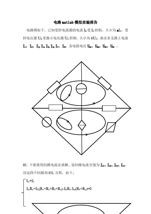
实验一:直流电路1.电阻电路的计算程序:1电阻电路的计算第1题%本题选用回路法,列出的方程为Z*I=U的形式,求出回路电流,然后进一步求解Z=[ 20 -12 0; %阻抗矩阵-12 32 -12;0 -12 18];U=[10 0 0]'; %电压向量I=inv(Z)*U; %回路电路向量i3=I(1)-I(2); %求i3u4=I(2)*8; %求u4u7=I(3)*2; %求u7fprintf('(1) i3= %8.4fA\n u4= %8.4fV\n U7= %8.4fV\n',i3,u4,u7)us=10/u4*4; %根据电路线性性质,由上题的u4变化的倍数求出usUb=[us 0 0]'; %变化后的电压向量Ib=inv(Z)*Ub; %变化后的回路电流向量ib3=Ib(1)-Ib(2); %变化后的i3ub7=Ib(3)*2; %变化后的u7fprintf('(2) us= %8.4fV\n i3= %8.4fA \n U7= %8.4fV\n',us,ib3,ub7)输出结果:(1) i3= 0.3571Au4= 2.8571VU7= 0.4762V(2) us= 14.0000Vi3= 0.5000AU7= 0.6667V2、求解电路里的电压程序:%导纳矩阵AA=[ 0.6 0.125 -0.125 -0.1 0 -5 01 -1 0 0 0 0 -100 -0.125 0.325 -0.2 0 0 00 0 1 -1 0 0 5-0.1 0 -0.2 0.55 -0.25 0 00 0 0 0 1 0 01 0 0 -1 0 -1 0];%电流矩阵BB=[0 0 5 0 0 24 0]';V=inv(A)*B;fprintf('V(1)=%f V\nV(2)=%f V\nV(3)=%f V\nV(4)=%f V\nV(5)=%f V\n',V(1),V(2),V(3),V(4),V(5));输出结果:V(1)=117.479167V(2)=299.770833V(3)=193.937500V(4)=102.791667V(5)=24.0000001.求解含有受控源的电路里的电流程序:%A为阻抗方程A=[ 0 0 1 0 0 04 0 -4 12 -4 -4-4 0 0 -4 8 00 0.5 0 0 0 10 -1 0 0 1 0-1 0 0 1 0 -1];B=[2 0 0 0 0 0]';%B为电压方程I=inv(A)*B;fprintf('i1= %.0f A\ni2= %.0f A\n',I(1),I(2));输出结果:i1= 1 Ai2= 1 A实验二:直流电路(2)1.求最大功率损耗程序:A=[ 1 0-1/10000 1/10000];is=0;B=[10 is]'x 104-3V=A\B; Uoc=V(2); is=1;B=[0 is]'; V=A\B;Req=[V(2)-V(1)]/is; Pmax=Uoc.^2/(4.*Req)fprintf('The maximum power occurs at %f ¦¸\n',Req) fprintf('The maximum powerdissipation is %f W',Pmax) RL=0:50000;VL=10.*RL./(10000+RL); PL=VL.^2./RL;figure(1),plot(RL,PL),grid输出结果:The maximum power occurs at 10000.000000 ΩThe maximum powerdissipation is 0.002500 W输出图形如下则从图上可验证当RL 为10K Ω时,最大功率约为2.5×W2. 求消耗的功率程序: A=[1 0 0 0-1/5 1/5+1/2+1/20 -1/2 0 0 -1/2 1/2+1/24+1/1.2 -1/1.2 0 0 -1/1.2 1/1.2]; V1=inv(A)*[75 0 0 0]'; Uoc=V1(4); is=1;V2=inv(A)*[0 0 0 is]'; Req=V2(4)/is;RL=[0 2 4 6 10 18 24 42 90 186];REQ=[Req Req Req Req Req Req Req Req Req Req];B=REQ+RL;for i=1:1:10;UL=Uoc.*RL(i)/B(i);IL=Uoc./B(i);PL=UL.*IL;fprintf('(%2d)',i);fprintf(' RL= %6.0f ¦¸',RL(i));fprintf(' IL= %6.3f A',IL);fprintf(' UL= %6.3f V',UL);fprintf(' PL= %6.3f W\n',PL);end输出结果:( 1) RL= 0 Ω IL= 8.000 A UL= 0.000 V PL= 0.000 W ( 2) RL= 2 Ω IL= 6.000 A UL= 12.000 V PL= 72.000 W( 3) RL= 4 Ω IL= 4.800 A UL= 19.200 V PL= 92.160 W( 4) RL= 6 Ω IL= 4.000 A UL= 24.000 V PL= 96.000 W( 5) RL= 10 Ω IL= 3.000 A UL= 30.000 V PL= 90.000 W( 6) RL= 18 Ω IL= 2.000 A UL= 36.000 V PL= 72.000 W( 7) RL= 24 Ω IL= 1.600 A UL= 38.400 V PL= 61.440 W( 8) RL= 42 Ω IL= 1.000 A UL= 42.000 V PL= 42.000 W( 9) RL= 90 Ω IL= 0.500 A UL= 45.000 V PL= 22.500 W(10) RL= 186 Ω IL= 0.250 A UL= 46.500 V PL= 11.625 W 实验三:正弦稳态1.求各支路的电流相量和电压相量程序:%设置变量R1=2;R2=3;R3=4;XL=2;XC1=3;XC2=5;Us1=8;Us2=6;Us3=8;Us4=15;%求阻抗Z1=(j*XL*R1)/(j*XL+R1);Z2=R2*(-j*XC1)/[(R2-j*XC1)];Z3=R3*(-j*XC2)/(R3-j*XC2);Y1=1/Z1;Y2=1/Z2;Y3=1/Z3;%导纳矩阵YY=[Y1+Y2 -Y2-Y2 Y2+Y3];%电流矩阵II=[Us1/(j*XL)+Us2/R2902701800 Us3/R3-Us4/(j*XC2)-Us2/R2]; U=inv(Y)*I;ua=U(1),ub=U(2),I1=ua*Y1,I2=(ub-ua)*Y2,I3=-ub*Y3, I1R=ua/R1,I1L=(ua)/(j*XL), I2R=-(ua-ub)/R2,I2C=-(ua-ub)/(-j*XC1), I3R=(ub)/R3, I3C=ub/(-j*XC2),compass([ua,ub,I1,I2,I3,I1R,I1L,I2R,I2C,I3R,I3C]); 输出结果:ua = 3.7232 - 1.2732i ub = 4.8135 + 2.1420iI1 = 1.2250 - 2.4982iI2 = -0.7750 + 1.5018i I3 = -0.7750 - 1.4982i I1R = 1.8616 - 0.6366i I1L = -0.6366 - 1.8616iI2R = 0.3634 + 1.1384i I2C = -1.1384 + 0.3634i I3R = 1.2034 + 0.5355i I3C = -0.4284 + 0.9627i输出图形为:2. 含互感的电路:复功率程序: %设置变量R1=4;R2=2;R3=2;XL1=10;XL2=8;XM=4;XC=8;US=10;IS=10;Z1=R1*(-j*XC)/(R1-j*XC);Z2=j*(XL1-XM);Z3=j*XM;Z4=j*(XL2-XM)+R2;Z5=R3;Y1=1/Z1;Y2=1/Z2;Y3=1/Z3;Y4=1/Z4;Y5=1/Z5;%导纳矩阵YY=[Y1+Y2 -Y2 0-Y2 Y2+Y3+Y4 -Y40 -Y4 Y4+Y5];I=[US/R1 0 IS]';U=inv(Y)*I;ua=U(1);ub=U(2);uc=U(3);i1=(US-ua)/R1;Pus=US*conj(i1),Pis=uc*conj(IS)输出结果:Pus = -4.0488 - 9.3830iPis = 1.7506e+02 + 3.2391e+01i3.正弦稳态电路:求未知参数程序:US=100;I1=0.1;P=6;XL1=1250;XC=750;P=6;Z1=j*XL1;Z2=-j*XC;cos_a=P/(US*I1);a=acos(cos_a);I1=0.1*exp(-a*1i);UL1=I1*Z1;UC2=US-UL1;IC2=UC2/Z2;IL3=I1-IC2;ZL=UC2/IL3;IC2=UC2/Z2;IZ3=I1-IC2;Z3=UC2/IZ3R3=real(Z3)XL3=imag(Z3)输出结果:Z3 = 7.5000e+02 + 3.7500e+02iR3 = 750.0000XL3 = 375.00004.正弦稳态电路,利用模值求解程序:%变量初始化syms XL;U2=200;IR=10;XC=10;R=U2/IR;%解方程的语句f=R*XL-sqrt((XC*XL)^2+[R*(XL-XC)]^2);XL=solve(f,XL);XL1=XL(1)XL2=XL(2)输出结果:XL1 = 20*3^(1/2) + 40XL2 = 40 - 20*3^(1/2)实验四:交流分析和网络函数1.求解电流和电压程序:%本程序计算回路电流I1,I2%Z是阻抗矩阵,U是电压向量,I是电流矩阵Z=[10-7.5i -6+5i-6+5i 16+3i];Zc=-10i;U1=5;U2=-2*exp(75i*pi/180);U=[U1 U2]';I=Z\U;I1_abs=abs(I(1));I1_ang=angle(I(1))*180/pi;Ic=I(1)-I(2);Uc=Ic*Zc;Uc_abs=abs(Uc);Uc_ang=angle(Uc)*180/pi;fprintf('current I1,magnitude: %f \n current I1,angle in degree:%f\n',I1_abs,I1_ang);fprintf('voltage Uc,magnitude: %f \n voltage Uc,angle in degree:%f\n',Uc_abs,Uc_ang);运行结果:current i1,magnitude: 0.387710current i1, angle in degree: 15.019255voltage vc,magnitude: 4.218263voltage vc,angle in degree:-40.8616912.求解三相不平衡相电压程序:%U为电压矩阵,I为电流矩阵,Z为总阻抗矩阵,ZL为负载阻抗矩阵U1=110;U2=110*exp(-120i*pi/180);U3=110*exp(120i*pi/180);U=[U1 U2 U3]';Z1=[6+13i 4+2i 6-12.5i]';ZL=[5+12i 3+4i 5-12i]';I=U./Z1;Vn=I.*ZL;Vna_abs=abs(Vn(1));Vna_ang=angle(Vn(1))*180/pi;Vnb_abs=abs(Vn(2));Vnb_ang=angle(Vn(2))*180/pi;Vnc_abs=abs(Vn(3));Vnc_ang=angle(Vn(3))*180/pi;fprintf('phasor vlotage Vna,magnitude:%f \n phasor voltage Vna,angle in dgree: %f \n',Vna_abs,Vna_ang);fprintf('phasor vlotage Vnb,magnitude:%f \n phasor voltage Vnb,angle in dgree: %f \n',Vnb_abs,Vnb_ang);fprintf('phasor vlotage Vnc,magnitude:%f \n phasor voltage Vnc,angle in dgree: %f \n',Vnc_abs,Vnc_ang);运行结果:phasor vlotage Vna,magnitude:99.875532phasor voltage Vna,angle in dgree: -2.155276phasor vlotage Vnb,magnitude:122.983739phasor voltage Vnb,angle in dgree: 93.434949phasor vlotage Vnc,magnitude:103.134238phasor voltage Vnc,angle in dgree: -116.978859实验五:动态电路1.正弦激励的一阶电路程序:%变量初始化R=2;C=0.5;Uc0=4;Um=10;Ulong=Um;%作图t=0:0.01:20;time=R*C;Uct=Ulong+(Uc0-Ulong)*exp(-t/time); figure(1),plot(t,Uct),grid运行结果:2.二阶欠阻尼电路的零输入响应程序:L=0.5;R=1;C=0.02;%输入元件参数 Uc0=1;IL0=0;alpha=R/2/L;wn=sqrt(1/(L*C));%输入给定参数 p1=-alpha+sqrt(alpha^-wn^2);%方程的两个根 p2=-alpha-sqrt(alpha^2-wn^2) dt=0.01;t=0:dt:1; %设定时间组 %用公式Uc1=(p2*Uc0-IL0/C)/(p2-p1)*exp(p1*t);%Uc 的第一个分量 Uc2=-(p1*Uc0-IL0/C)/(p2-p1)*exp(p2*t);%Uc 的第二个分量 IL1=p1*C*(p2*Uc0-IL0/C)/(p2-p1)*exp(p1*t); IL2=-p2*C*(p1*Uc0-IL0/C)/(p2-p1)*exp(p2*t); Uc=Uc1+Uc2; IL=IL1+IL2;%分别画出两种数据曲线subplot(2,1,1),plot(t,Uc),grid subplot(2,1,2),plot(t,IL),grid运行结果:0246810121416182045678910R=1R=200.10.20.30.40.50.60.70.80.91-1-0.500.5100.10.20.30.40.50.60.70.80.910.511.52R=300.10.20.30.40.50.60.70.80.91-0.06-0.04-0.0200.0200.10.20.30.40.50.60.70.80.9100.20.40.60.81R=400.10.20.30.40.50.60.70.80.91-0.06-0.04-0.0200.0200.10.20.30.40.50.60.70.80.9100.20.40.60.8100.10.20.30.40.50.60.70.80.91-0.08-0.06-0.04-0.0200.0200.10.20.30.40.50.60.70.80.9100.20.40.60.81R=60.10.20.30.40.50.60.70.80.91-0.08-0.06-0.04-0.0200.0200.10.20.30.40.50.60.70.80.9100.20.40.60.8100.10.20.30.40.50.60.70.80.91-0.08-0.06-0.04-0.0200.0200.10.20.30.40.50.60.70.80.9100.20.40.60.81R=80.10.20.30.40.50.60.70.80.91-0.08-0.06-0.04-0.0200.0200.10.20.30.40.50.60.70.80.9100.20.40.60.8100.10.20.30.40.50.60.70.80.91-0.08-0.06-0.04-0.0200.0200.10.20.30.40.50.60.70.80.91-0.50.51R=100.10.20.30.40.50.60.70.80.91-0.08-0.06-0.04-0.0200.0200.10.20.30.40.50.60.70.80.91-0.50.5100.10.20.30.40.50.60.70.80.91-0.08-0.06-0.04-0.02000.10.20.30.40.50.60.70.80.9100.20.40.60.81实验六:频率响应1.一阶低通电路的频率响应程序:ww=0:0.2:4;%设定频率数组 ww=w/wcH=1./(i+j*ww);%求复频率响应figure(1)subplot(2,1,1),plot(ww,abs(H)),%绘制幅频特性grid,xlabel('ww'),ylabel('angle(H)')subplot(2,1,2),plot(ww,angle(H)),%绘制相频特性grid,xlabel('ww'),ylabel('angle(H)')figure(2) %绘制对数频率特性subplot(2,1,1),semilogx(ww,20*log10(abs(H)))%纵坐标为分贝grid,xlabel('ww'),ylabel('分贝')subplot(2,1,2),semilogx(ww,angle(H))%绘制相频特性grid,xlabel('ww'),ylabel('angle(H)')运行结果:00.51 1.52 2.53 3.540.20.40.60.81wwa n g l e (H )0.511.52 2.533.54-3-2.5-2-1.5-1-0.5wwa n g l e (H )100ww分贝10wwa n g l e (H )2.频率响应:二阶低通电路程序:for Q=[1/3,1/2,1/sqrt(2),1,2,5]ww=logspace(-1,1,50);%设无量纲频率数组ww=w/w0H=1./(1+j*ww/Q+(j*ww).^2);%求复频率响应figure(1)subplot(2,1,1),plot(ww,abs(H)),hold onsubplot(2,1,2),plot(ww,angle(H)),hold onfigure(2)subplot(2,1,1),semilogx(ww,20*log10(abs(H))),hold on%纵坐标为分贝subplot(2,1,2),semilogx(ww,angle(H)),hold on%绘制相频特性endfigure(1),subplot(2,1,1),grid,xlabel('w'),ylabel('abs(H)')subplot(2,1,2),grid,xlabel('w'),ylabel('angle(H)')figure(2),subplot(2,1,1),grid,xlabel('w'),ylabel('abs(H)')subplot(2,1,2),grid,xlabel('w'),ylabel('abs(H)')运行结果:012345678910246wa b s (H )012345678910-4-3-2-10wa n g l e (H )3. 频率响应:二阶带通电路程序:clear,format compact H0=1;wn=1;for Q=[5,10,20,50,100]w=logspace(-1,1,50);%设频率数组w H=H0./(1+j*Q*(w./wn-wn./w)); figure(1)%横坐标为线性坐标subplot(2,1,1),plot(w,abs(H)),grid,hold on %绘制幅频特性 subplot(2,1,2),plot(w,angle(H)),grid,hold on %绘制相频特性 figure(2)subplot(2,1,1),semilogx(w,20*log10(abs(H))),grid,hold on %纵坐标为分贝subplot(2,1,2),semilogx(w,angle(H)),grid,hold on %绘制相频特性 end运行结果:10-1100101-60-40-20020wa b s (H )10-1100101-4-3-2-10wa b s (H )01234567891000.20.40.60.81012345678910-2-112复杂谐振电路的计算程序:clear,format compactR1=2;R2=3;L1=0.75e-3;L2=0.25e-3;C=1000e-12;Rs=28200;L=L1+L2;R=R1+R2;Rse=Rs*(L/L1)^2%折算内阻f0=1/(2*pi*sqrt(C*L))Q0=sqrt(L/C)/R,R0=L/C/R;%空载Q0值Re=R0*Rse/(R0+Rse)%折算内阻与回路电阻的并联Q=Q0*Re/R0,B=f0/Q,%实际Q 值和带通s=log10(f0);f=logspace(s-.1,s+.1,501);w=2*pi*f;%设定计算的频率及范围及数组 z1e=R1+j*w*L;z2e=R2+1./(j*w*C);%等效单回路中量纲电抗支路的阻抗 ze=1./(1./z1e+1./z2e+1./Rse);%等效回路中三个支路的并联阻抗subplot(2,1,1),loglog(w,abs(ze)),grid%画对数幅频特性axis([min(w),max(w),0.9*min(abs(ze)),1.1*max(abs(ze))]) 10-1100101-60-40-202010-1100101-2-112subplot(2,1,2),semilogx(w,angle(ze)*180/pi)axis([min(w),max(w),-100,100]),gridfh=w(find(abs(1./(1./z1e+1./z2e))>50000))/2/pi;%求回路阻抗大于50千欧的频带fhmin=min(fh),fhmax=max(fh)运行结果:10610106。