宏观经济学 曼昆 习题答案 章节9

第9章经济增长Ⅱ：技术、经验和政策一、概念题1．劳动效率（efficiency of labor）答：劳动效率是指单位劳动时间的产出水平，反映了社会对生产方法的掌握和熟练程度。

当可获得的技术改进时，劳动效率会提高。

当劳动力的健康、教育或技能得到改善时，劳动效率也会提高。

在索洛模型中，劳动效率（E）是表示技术进步的变量，反映了索洛模型劳动扩张型技术进步的思想：技术进步提高了劳动效率，就像增加了参与生产的劳动力数量一样，所以在生产函数中的劳动力数量上乘以一个劳动效率变量，形成了有效工人概念，这使得索洛模型在稳态分析中纳入了外生的技术进步。

2．劳动改善型技术进步（labor-augmenting technological progress）答：劳动改善型技术进步是指技术进步提高了劳动效率，就像增加了参与生产的劳动力数量一样，所以在生产函数中的劳动力数量上乘以一个劳动效率变量，以反映外生技术进步对经济增长的影响。

劳动改善型技术进步实际上认为技术进步是通过提高劳动效率而影响经济增长的。

它的引入形成了有效工人的概念，从而使得索洛模型能够以单位有效工人的资本和产量来进行稳定状态研究。

3．内生增长理论（endogenous growth theory）答：内生增长理论是用规模收益递增和内生技术进步来说明一个国家长期经济增长和各国增长率差异的一种经济理论，其重要特征就是试图使增长率内生化。

根据其依赖的基本假定条件的差异，可以将内生增长理论分为完全竞争条件下的内生增长模型和垄断竞争条件下的内生增长模型。

按照完全竞争条件下的内生增长模型，使稳定增长率内生化的两条基本途径就是：①将技术进步率内生化；②如果可以被积累的生产要素有固定报酬，那么可以通过某种方式使稳态增长率受要素的积累影响。

内生增长理论是抛弃了索洛模型外生技术进步的假设，以更好地研究技术进步与经济增长之间的关系的理论。

它认为经济增长是可以内生持续的，不会达到索洛模型的稳定状态。

曼昆《宏观经济学》（第9版）章节习题精编详解第2篇古典理论：长期中的经济第7章失业一、概念题1．自然失业率（natural rate of unemployment）答：自然失业率又称“有保证的失业率”、“正常失业率”、“充分就业失业率”等，它是经济围绕其波动的平均失业率，是经济在长期中趋近的失业率，是充分就业时仍然保持的失业水平。

自然失业率是在没有货币因素干扰的情况下，让劳动市场和商品市场自发供求力量起作用时，总供给和总需求处于均衡状态时的失业率。

“没有货币因素干扰”是指失业率的高低与通货膨胀率的高低之间不存在替代关系。

自然失业率决定于经济中的结构性和摩擦性的因素，取决于劳动市场的组织状况、人口组成、失业者寻找工作的能力愿望、现有工作的类型、经济结构的变动、新加入劳动者队伍的人数等众多因素。

任何把失业降低到自然失业率以下的企图都将造成加速的通货膨胀。

任何时候都存在着与实际工资率结构相适应的自然失业率。

自然失业率是弗里德曼对菲利普斯曲线发展的一种观点，他将长期的均衡失业率称为“自然失业率”，它可以和任何通货膨胀水平相对应，且不受其影响。

2．摩擦性失业（frictional unemployment）答：摩擦性失业指劳动力市场运行机制不完善或者因为经济变动过程中的工作转换而产生的失业。

摩擦性失业是劳动力在正常流动过程中所产生的失业。

在一个动态经济中，各行业、各部门和各地区之间劳动需求的变动是经常发生的。

即使在充分就业状态下，由于人们从学校毕业或搬到新城市而要寻找工作，总是会有一些人的周转。

摩擦性失业量的大小取决于劳动力流动性的大小和寻找工作所需要的时间。

由于在动态经济中，劳动力的流动是正常的，所以摩擦性失业的存在也是正常的。

3．部门转移（sectoral shift）答：部门转移是指劳动力在不同部门和行业的重新配置。

由于许多原因，企业和家庭需要的产品类型一直在变动。

随着产品需求的变动，对生产这些产品的劳动力的需求也在改变，因此就出现劳动力在部门之间的转移。

第4篇 经济周期理论：短期中的经济第9章 经济波动导论课后习题详解跨考网独家整理最全经济学考研真题，经济学考研课后习题解析资料库，您可以在这里查阅历年经济学考研真题，经济学考研课后习题，经济学考研参考书等内容，更有跨考考研历年辅导的经济学学哥学姐的经济学考研经验，从前辈中获得的经验对初学者来说是宝贵的财富，这或许能帮你少走弯路，躲开一些陷阱。

以下内容为跨考网独家整理，如您还需更多考研资料，可选择经济学一对一在线咨询进行咨询。

一、概念题1．奥肯定律（Okun ’s law ）答：奥肯定律是表示失业率与实际国民收入增长率之间关系的经验统计规律，由美国经济学家奥肯在20世纪60年代初提出。

其主要内容是：失业率每高于自然失业率1个百分点，实际GDP 将低于潜在GDP 2个百分点。

奥肯定律的一个重要结论是：实际GDP 必须保持与潜在GDP 同样快的增长，以防止失业率的上升。

如果政府想让失业率下降，那么，该经济社会的实际GDP 的增长必须快于潜在GDP 的增长。

根据奥肯的研究，在美国，失业率每下降1%，实际国民收入增长2%。

但应该指出的是：①奥肯定律表明了失业率与实际国民收入增长率之间是反方向变动的关系；②两者的数量关系1∶2是一个平均数，在不同的时期，这一比率并不完全相同；③这一规律适用于经济没有实现充分就业时的情况。

在经济实现了充分就业时，这一规律所表示的自然失业率与实际国民收入增长率之间的关系要弱得多，一般估算是1∶0.76。

2．领先指标（leading indicators ）答：领先指标是指一般先于整体经济变动的变量，可以帮助经济学家预测短期经济波动。

由于经济学家对前导指标可靠意见看法的不一致，导致经济学家给出不同的预测，其中就包括短期经济波动情况的预测。

领先指标的大幅度下降预示经济很可能会衰退，大幅度上升预示经济很可能会繁荣。

3．总需求（aggregate demand ）答：总需求是指整个经济社会在任何一个给定的价格水平下对产品和劳务的需求总量。

第1章宏观经济学科学一、概念题1．宏观经济学（macroeconomics）答：宏观经济学与微观经济学相对，是一种现代的经济分析方法。

它以国民经济总体作为考察对象，研究经济生活中有关总量的决定与变动，解释失业、通货膨胀、经济增长与波动、国际收支及汇率的决定与变动等经济中的宏观整体问题，所以又称之为总量经济学。

宏观经济学的中心和基础是总需求—总供给模型。

具体来说，宏观经济学主要包括总需求理论、总供给理论、失业与通货膨胀理论、经济增长与经济周期理论、开放经济理论、宏观经济政策等内容。

对宏观经济问题进行分析与研究的历史十分悠久，但现代意义上的宏观经济学直到20世纪30年代才得以形成和发展起来。

现代宏观经济学诞生的标志是凯恩斯于1936年出版的《就业、利息和货币通论》。

宏观经济学在20世纪30年代奠定基础，二战后逐步走向成熟并得到广泛应用，20世纪60年代后的“滞胀”问题使凯恩斯主义的统治地位受到严重挑战并形成了货币主义、供给学派、理性预期等学派对立争论的局面，20世纪90年代新凯恩斯主义的形成又使国家干预思想占据主流。

宏观经济学是当代发展最为迅猛，应用最为广泛，因而也是最为重要的经济学学科。

2．实际GDP（real GDP）答：实际GDP指用以前某一年的价格作为基期的价格计算出来的当年全部最终产品的市场价值。

它衡量在两个不同时期经济中的产品产量变化，以相同的价格或不变金额来计算两个时期所生产的所有产品的价值。

在国民收入账户中，以2010年的价格作为基期来计算实际GDP，意味着在计算实际GDP时，用现期的产品产量乘以2010年的价格，便可得到以2010年价格出售的现期产出的价值。

3．通货膨胀与通货紧缩（inflation and deflation）答：（1）通货膨胀是指在一段时期内，一个经济中大多数商品和劳务的价格水平持续显著地上涨。

它包含三层含义：①通货膨胀是经济中一般价格水平的上涨，而不是个别商品或劳务的价格上涨；②通货膨胀是价格的持续上涨，而非一次性上涨；③通货膨胀是价格的显著上涨，而非某些微小的上升，例如每年上升0.5%，不能视为通货膨胀。

思考与练习1．名词解释需求管理政策供给管理政策财政预算财政政策货币政策自动稳定器法定准备金率货币乘数基础货币再贴现公开市场业务政策效应财政财政效应货币政策效应挤出效应双松政策双紧政策2．试述宏观经济政策的目标及其相互关系。

3．功能财政思想与平衡预算的财政思想有何区别？4．试述财政政策的自动稳定器功能？是否税率越高，税收作为自动稳定器的作用越大? 5．什么是权衡性的财政政策?如何操作?6．什么是货币乘数，它是如何起作用的？7．说明货币政策的传导机制与内容。

8．中央银行的货币政策工具主要有哪些？9．试述货币创造乘数及影响因素.10．试述财政政策效果及影响因素。

11．试述货币政策效果及影响因素。

12．试述货币财政政策挤出效应的制约因素.13．什么是挤出效应？挤出效应的制约因素有哪些？14．试述货币政策的局限性。

15．画图说明IS曲线斜率对财政政策效果的影响。

16．画图说明LM曲线斜率对财政政策效果的影响.17．画图说明IS曲线斜率对货币政策效果的影响。

18．画图说明LM曲线斜率对货币政策效果的影响。

19．试述财政政策和货币政策配合使用具体有哪几种方式？20．货币是否存在挤出效应?为什么?21．画图说明双松的政策效应。

22．画图说明双紧的政策效应。

23．画图说明财政松货币紧的政策效应。

24．画图说明财政紧货币松的政策效应。

25．假定经济起初处于充分就业状态，现在政府要改变总需求构成,增加私人投入而减少消费支出，但不改变总需求水平，试问应当实行一种什么样的混合政策？并用IS-LM图形表示这一政策建议。

25．假定政府要削减税收，试用IS-LM模型表示以下两种情况下减税的影响：（1)用适应性货币政策保持利率不变。

（2）货币存量不变.1．名词解释（1）需求管理政策：指通过调节总需求来达到一定宏观经济目标的政策措施。

（2)供给管理政策:通过调节总供给来达到一定的宏观经济目标的政策措施。

（3)财政预算：指政府逐年估算未来财政年度的收入与支出，以促进宏观经济目标的实现。

宏观经济学课后习题答案(共9篇)宏观经济学课后习题答案（一）: 这是曼昆的宏观经济学的24章的课后习题，求高手解答，我要详细的计算过程！答案我已经知道，是变动0.4美元在长期中，糖果的价格从0．10美元上升到0．60美元。

在同一时期中，消费物价指数从150上升到300。

根据整体通货膨胀进行调整后，糖果的价格变动了多少我要详细的解答过程，怎么算的就行了！由CPI可知，通货膨胀率=（300-150）/150*100%=100%糖果的原始价格P=0.1在这段时间通过通货膨胀变为0.1*（1+通货膨胀率）=0.2实际上糖果在后来卖到了0.6，所以糖果实际价格变动了0.6-0.2=0.4美元宏观经济学课后习题答案（二）: 曼昆宏观经济学26章课后题答案是不是错了假设政府明年借债比今年多了200亿美元,对于可贷资金市场的利率和投资,供给和需求曲线的变动,答案是不是有错答案说是供给曲线不变,需求曲线右移,我认为是需求曲线不动,供给曲线左移……财政政策当然变动的是需求,供给怎么可能变动,你可能是总供给和总需求有些混淆,我开始的时候也不是很清楚,多看几遍就明白了,供给曲线可能因为劳动力变动,而合财政货币政策无关.这些政策变动的都是需求.另外右移就是借钱多了,就是投资需求多了,就是G多了,那就是需求曲线右移了宏观经济学课后习题答案（三）: 谁有高鸿业版《西方经济学》宏观部分——第十七章课后题答案第十七章总需求——总供给模型1、（1）总需求是经济社会对产品和劳务的需求总量,这一需求总量通常以产出水平来表示.一个经济社会的总需求包括消费需求、投资需求、.政府购买和国外需求.总需求量受多种因素的影响,其中价格水平是一个重要的因素.在宏观经济学中,为了说明价格对总需求量的影响,引入了总需求曲线的概念,即总需求量与价格水平之间关系的几何表示.在凯恩斯主义的总需求理论中,总需求曲线的理论来源主要由产品市场均衡理论和货币市场均衡理论来反映.（2）在IS—LM模型中,一般价格水平被假定为一个常数（参数）.在价格水平固定不变且货币供给为已知的情况下,IS曲线和LM曲线的交点决定均衡的收入水平.现用图1—62来说明怎样根据IS—LM图形推导总需求曲线.图1—62分上下两部.上图为IS—LM图.下图表示价格水平和需求总量之间的关系,即总需求曲线.当价格P的数值为时,此时的LM曲线与IS曲线相交于点 , 点所表示的国民收入和利率顺次为和 .将和标在下图中便得到总需求曲线上的一点 .现在假设P由下降到 .由于P的下降,LM曲线移动到的位置,它与IS曲线的交点为点. 点所表示的国民收入和利率顺次为和 .对应于上图的点 ,又可在下图中找到 .按照同样的程序,随着P的变化,LM曲线和IS曲线可以有许多交点,每一个交点都代表着一个特定的y和p.于是有许多P与的组合,从而构成了下图中一系列的点.把这些点连在一起所得到的曲线AD便是总需求曲线.从以上关于总需求曲线的推导中看到,总需求曲线表示社会中的需求总量和价格水平之间的相反方向的关系.即总需求曲线是向下方倾斜的.向右下方倾斜的总需求曲线表示,价格水平越高,需求总量越小；价格水平越低,需求总量越大.2、财政政策是政府变动税收和支出,以便影响总需求,进而影响就业和国民收入的政策.货币政策是指货币当局即中央银行通过银行体系变动货币供应量来调节总需求的政策.无论财政政策还是货币政策,都是通过影响利率、消费和投资进而影响总需求,使就业和国民收入得到调节的,通过对总需求的调节来调控宏观经济,所以称为需求管理政策.3、总供给曲线描述国民收入与一般价格水平之间的依存关系.根据生产函数和劳动力市场的均衡推导而得到.资本存量一定时,国民收入水平碎就业量的增加而增加,就业量取决于劳动力市场的均衡.所以总供给曲线的理论来源于生产函数和劳动力市场均衡的理论.4、总供给曲线的理论主要由总量生产函数和劳动力市场理论来反映的.在劳动力市场理论中,经济学家对工资和价格的变化和调整速度的看法是分歧的.古典总供给理论认为,劳动力市场运行没有阻力,在工资和价格可以灵活变动的情况下,劳动力市场得以出清,使经济的就业总能维持充分就业状态,从而在其他因素不变的情况下,经济的产量总能保持在充分就业的产量或潜在产量水平上.因此,在以价格为纵坐标,总产量为横坐标的坐标系中,古典供给曲线是一条位于充分就业产量水平的垂直线.凯恩斯的总供给理论认为,在短期,一些价格是粘性的,从而不能根据需求的变动而调整.由于工资和价格粘性,短期总供给曲线不是垂直的,凯恩斯总供给曲线在以价格为纵坐标,收入为横坐标的坐标系中是一条水平线,表明经济中的厂商在现有价格水平上,愿意供给所需的任何数量的商品.作为凯恩斯总供给曲线基础的思想是,作为工资和价格粘性的结果,劳动力市场不能总维持在充分就业状态,由于存在失业,厂商可以在现行工资下获得所需劳动.因而他们的平均生产成本被认为是不随产出水平变化而变化.一些经济学家认为,古典的和凯恩斯的总供给曲线分别代表着劳动力市场的两种极端的说法.在现实中工资和价格的调整经常介于两者之间.在这种情况下以价格为纵坐标,产量为横坐标的坐标系中,总供给曲线是向右上方延伸的,这即为常规的总需求曲线.总之,针对总量劳动市场关于工资和价格的不同假设,宏观经济学中存在着三种类型的总供给曲线.5、解答：宏观经济学在用总需求—总供给说明经济中的萧条,高涨和滞涨时,主要是通过说明短期的收入和价格水平的决定来完成的.如图1—63所示. 从图1—63可以看到,短期的收入和价格水平的决定有两种情况.第一种情况是,AD是总需求曲线, 使短期供给曲线,总需求曲线和短期供给曲线的交点E决定的产量或收入为y,价格水平为P,二者都处于很低的水平,第一种情况表示经济处于萧条状态.第二种情况是,当总需求增加,总需求曲线从AD向右移动到时,短期总供给曲线和新的总需求曲线的交点决定的产量或收入为 ,价格水平为 ,二者都处于很高的水平,第二种情况表示经济处于高涨状态.现在假定短期供给曲线由于供给冲击（如石油价格和工资等提高）而向左移动,但总需求曲线不发生变化.在这种情况下,短期收入和价格水平的决定可以用图1—64表示.在图1—64中,AD是总需求曲线,是短期总供给曲线,两者的交点E决定的产量或收入为,价格水平为P.现在由于出现供给冲击,短期总供给曲线向左移动到,总需求曲线和新的短期总供给曲线的交点决定的产量或收入为,价格水平为,这个产量低于原来的产量,而价格水平却高于原来的价格水平,这种情况表示经济处于滞涨状态,即经济停滞和通货膨胀结合在一起的状态.6、二者在“形式”上有一定的相似之处.微观经济学的供求模型主要说明单个商品的价格和数量的决定.宏观经济中的AD—AS模型主要说明总体经济的价格水平和国民收入的决定.二者在图形上都用两条曲线来表示,在价格为纵坐标,数量为横坐标的坐标系中,向右下方倾斜的为需求曲线,向右上方延伸的为供给曲线.但二者在内容上有很大的不同：其一,两模型涉及的对象不同.微观经济学的供求模型是微观领域的事物,而宏观经济中的AD—AS模型是宏观领域的事物.其二,各自的理论基础不同.微观经济学中的供求模型中的需求曲线的理论基础是消费者行为理论,而供给曲线的理论基础主要是成本理论和市场理论,它们均属于微观经济学的内容.宏观经济学中的总需求曲线的理论基础主要是产品市场均衡和货币市场均衡理论,而供给曲线的理论基础主要是劳动市场理论和总量生产函数,它们均属于宏观经济学的内容.其三,各自的功能不同.微观经济学中的供求模型在说明商品的价格和数量的决定的同时,还可以来说明需求曲线和供给曲线移动对价格和商品数量的影响,充其量这一模型只解释微观市场的一些现象和结果.宏观经济中的AD—AS模型在说明价格和产出决定的同时,可以用来解释宏观经济的波动现象,还可以用来说明政府运用宏观经济政策干预经济的结果.7、（1）由得；2023 + P = 2400 - P于是 P=200, =2200即得供求均衡点.（2）向左平移10%后的总需求方程为：于是,由有：2023 + P = 2160 – PP=80 , =2080与（1）相比,新的均衡表现出经济处于萧条状态.（3）向右平移10%后的总需求方程为：于是,由有：2023 + P = 2640 – PP=320 , =2320与（1）相比,新的均衡表现出经济处于高涨状态.（4）向左平移10%后的总供给方程为：于是,由有：1800 + P = 2400 – PP=300 , =2100与（1）相比,新的均衡表现出经济处于滞涨状态.（5）总供给曲线向右上方倾斜的直线,属于常规型.宏观经济学课后习题答案（四）: 宏观经济学问题题号:11 题型:单选题（请在以下几个选项中选择唯一正确答案）本题分数:5内容:一般把经济周期分为四个阶段,这四个阶段为（）.选项:a、兴旺,停滞,萧条和复苏b、繁荣,停滞,萧条和恢复c、繁荣,衰退,萧条和复苏d、兴旺,衰退,萧条和恢复题号:12 题型:单选题（请在以下几个选项中选择唯一正确答案）本题分数:5内容:“面粉是中间产品”这一命题（）选项:a、一定是对的b、一定是不对的c、可能是对的也可能是不对的d、以上三种说法全对.题号:13 题型:单选题（请在以下几个选项中选择唯一正确答案）本题分数:5内容:下列哪种情况下执行财政政策的效果较好（选项:a、LM陡峭而IS平缓b、LM平缓而IS陡峭c、LM和IS一样平缓d、LM和IS一样陡峭题号:14 题型:单选题（请在以下几个选项中选择唯一正确答案）本题分数:5内容:政府财政政策通过哪一个变量对国民收入产生影响（）.选项:a、进口b、消费支出c、出口d、政府购买.题号:15 题型:单选题（请在以下几个选项中选择唯一正确答案）本题分数:5内容:在国民收入核算体系中,计入GDP的政府支出是指（）.选项:a、政府购买物品的支出b、政府购买物品和劳务的支出c、政府购买物品和劳务的支出加上政府的转移支出之和d、政府工作人员的薪金和政府转移支出题号:16 题型:是非题本题分数:5内容:长期总供给曲线所表示的总产出是经济中的潜在产出水平选项:1、错2、对题号:17 题型:是非题本题分数:5内容:GDP中扣除资本折旧,就可以得到NNP选项:1、错2、对题号:18 题型:是非题本题分数:5内容:在长期总供给水平,由于生产要素等得到了充分利用,因此经济中不存在失业选项:1、错2、对题号:19 题型:是非题本题分数:5内容:个人收入即为个人可支配收入,是人们可随意用来消费或储蓄的收入选项:1、错2、对题号:20 题型:是非题本题分数:5内容:GNP折算指数是实际GDP与名义GDP的比率选项:1、错2、对C,C,A,D,B对,对（NNP国民生产净值）,错（可能还有摩擦失业）,错,错宏观经济学课后习题答案（五）: 一道宏观经济学的习题，求答案及解析7、将一国经济中所有市场交易的货币价值进行加总a、会得到生产过程中所使用的全部资源的市场价值b、所获得的数值可能大于、小于或等于GDP的值c、会得到经济中的新增价值总和d、会得到国内生产总值`b 正确市场交易的可能有中间产品，如此中间产品加上最终产品，则重复计算的结果大于GDP;不在国内市场交易，出口销往国外的漏算，则计算结果会小于gdp；如果重复的和漏算的正好相等，则结果可能等于gdp。

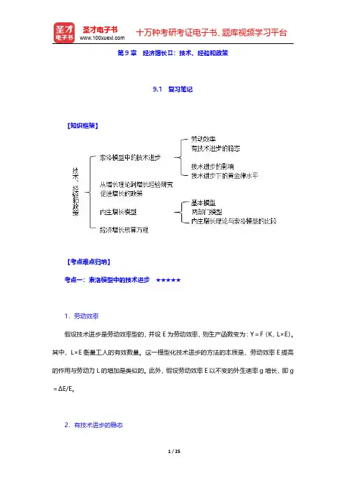
第9章经济增长Ⅱ：技术、经验和政策9.1复习笔记【知识框架】【考点难点归纳】考点一：索洛模型中的技术进步★★★★★1．劳动效率假设技术进步是劳动效率型的，并设E为劳动效率，则生产函数变为：Y＝F（K，L×E）。

其中，L×E衡量工人的有效数量。

这一模型化技术进步的方法的本质是，劳动效率E提高的作用与劳动力L的增加是类似的。

此外，假设劳动效率E以不变的外生速率g增长，即g ＝ΔE/E。

2．有技术进步的稳态设y＝Y/（L×E），k＝K/（L×E），对生产函数两边同除以L×E，可得单位效率工人产出函数，即y＝f（k）。

该函数形式虽然与上一章完全相同，但是意义已经发生了改变。

因为单位效率工人的储蓄（投资）为：sy＝sf（k），而单位效率工人的补偿投资（资本扩展化）为：（δ＋n＋g）k。

因此，当单位效率工人的储蓄和补偿投资相等时，即Δk＝sf （k）－（δ＋n＋g）k＝0，经济达到稳定状态。

如图9-1所示，k*表示稳态的资本存量，在这一水平，有效工人的人均资本和有效工人的人均产出保持不变。

图9-1技术进步和索洛模型3．技术进步的影响（见表9-1）表9-1技术进步的影响4．技术进步下的黄金律水平因为c*＝y*－i*＝f（k*）－（δ＋n＋g）k*，当c*达到最大化时，有：MPK＝δ＋n＋g 或MPK－δ＝n＋g。

这说明，在黄金律资本水平，资本的边际产出减去折旧率等于人口增长率与技术进步的和。

由于现实经济既有人口增长，又有技术进步，所以，必须用这个标准来评价经济的资本存量与黄金律稳态水平的关系。

考点二：从增长理论到增长经验研究★1．平衡的增长平衡的增长是指技术进步引起许多变量在稳态的数值一起上升。

根据索洛模型，在稳态，人均产出Y/L和人均资本存量K/L以技术进步的速率g增长。

技术进步也影响要素价格。

在稳态，实际工资以技术进步的速率增长。

而资本的实际租赁价格随着时间的推移是不变的。

曼昆宏观经济经济学第九版英文原版答案完整版曼昆宏观经济经济学第九版英文原版答案集团标准化办公室：[VV986T-J682P28-JP266L8-68PNN]A n s w e r s t o T e x t b o o k Q u e s t i o n s a n d P r o b l e m sCHAPTER 7Unemployment and the Labor MarketQuestions for Review1. The rates of job separation and job finding determine the naturalrate of unemployment. The rate of job separation is the fraction of people who lose their job each month. The higher the rate of jobseparation, the higher the natural rate of unemployment. The rate of job finding is the fraction of unemployed people who find a job each month. The higher the rate of job finding, the lower the natural rate of unemployment.2. Frictional unemployment is the unemployment caused by the time ittakes to match workers and jobs. Finding an appropriate job takes time because the flow of information about job candidates and job vacancies is not instantaneous. Because different jobs requiredifferent skills and pay different wages, unemployed workers may not accept the first job offer they receive.In contrast, structural unemployment is the unemployment resulting from wage rigidity and job rationing. These workers are unemployed not because they are actively searching for a job that best suits their skills (as in the case of frictional unemployment), but because at the prevailing real wage thequantity of labor supplied exceeds the quantity of labor demanded. If the wage does not adjust to clear the labor market, then these workers must wait for jobs to become available. Structural unemployment thus arises because firms fail to reduce wages despite an excess supply of labor.3. The real wage may remain above the level that equilibrates laborsupply and labor demand because of minimum wage laws, the monopoly power of unions, and efficiency wages.Minimum-wage laws cause wage rigidity when they prevent wages from falling to equilibrium levels. Although most workers are paid a wage above the minimum level, for some workers, especially the unskilled and inexperienced, the minimum wage raises their wage above theequilibrium level. It therefore reduces the quantity of their labor that firms demand, and creates an excess supply of workers, which increases unemployment.The monopoly power of unions causes wage rigidity because the wages of unionized workers are determined not by the equilibrium of supply and demand but by collective bargaining between union leaders and firm management. The wage agreement often raises the wage abovethe equilibrium level and allows the firm to decide how many workers to employ. These high wages cause firms to hire fewer workers than at the market-clearing wage, so structural unemployment increases.Efficiency-wage theories suggest that high wages make workers more productive. The influence of wages on worker efficiency may explain why firms do not cut wages despite an excess supply of labor. Even though a wage reduction decreasesthe firm’s wage bill, it may also lower worker productivity and therefore the firm’s profits.4. Depending on how one looks at the data, most unemployment can appearto be either short term or long term. Most spells of unemployment are short; that is, most of those who became unemployed find jobs quickly.On the other hand, most weeks of unemployment are attributable to the small number of long-term unemployed. By definition, the long-term unemployed do not find jobs quickly, so they appear on unemployment rolls for many weeks or months.5. Europeans work fewer hours than Americans. One explanation is thatthe higher income tax rates in Europe reduce the incentive to work. A second explanation is a larger underground economy in Europe as aresult of more people attempting to evade the high tax rates.A third explanation is the greater importance of unions in Europe and their ability to bargain for reduced work hours. A final explanation isbased on preferences, whereby Europeans value leisure more thanAmericans do, and therefore elect to work fewer hours.Problems and Applications1. a. In the example that follows, we assume that during the school yearyou look for a part-time job, and that, on average, it takes 2 weeks to find one. We also assume that the typical job lasts 1semester, or 12 weeks.b. If it takes 2 weeks to find a job, then the rate of job finding in weeks isf = (1 job/2 weeks) = 0.5 jobs/week.If the job lasts for 12 weeks, then the rate of job separation in weeks iss = (1 job/12 weeks) = 0.083 jobs/week.c. From the text, we know that the formula for the natural rate of unemployment is(U/L) = [s/(s + f )],where U is the number of people unemployed, and L is the number of people in the labor force.Plugging in the values for f and s that were calculated in part (b), we find(U/L) = [0.083/(0.083 + 0.5)] = 0.14.Thus, if on average it takes 2 weeks to find a job that lasts 12 weeks, the natural rate of unemployment for this population ofcollege students seeking part-time employment is 14 percent.2. Call the number of residents of the dorm who are involved I, thenumber who are uninvolved U, and the total number of students T = I + U. In steady state the total number of involved students is constant.For this to happen we need the number of newly uninvolved students,(0.10)I, to be equal to the number of students who just becameinvolved, (0.05)U. Following a few substitutions:(0.05)U = (0.10)I= (0.10)(T – U),soWe find that two-thirds of the students are uninvolved.3. To show that the unemployment rate evolves over time to thesteady-state rate, let’s begin by defining how the number of people unemployed changes over time. The change in the number of unemployed equals the number of people losing jobs (sE) minus the number finding jobs (fU). In equation form, we can express this as:U–U t= ΔU t + 1 = sE t–fU t.t + 1Recall from the text that L = E t + U t, or E t = L –U t, where L is the total labor force (we will assume that L is constant). Substituting for E t in the above equation, we findΔU t + 1 = s(L –U t) –fU t.Dividing by L, we get an expression for the change in the unemployment rate from t to t + 1:ΔU t + 1/L = (U t + 1/L) –(U t/L) = Δ[U/L]t + 1 = s(1 –U t/L) –fU t/L.Rearranging terms on the right side of the equation above, we end up with line 1 below. Now take line 1 below, multiply the right side by (s + f)/(s + f) and rearrange terms to end up with line 2 below:Δ[U/L]t + 1= s – (s + f)U t/L= (s + f)[s/(s + f) – U/L].tThe first point to note about this equation is that in steady state, when the unemployment rate equals its natural rate, the left-handside of this expression equals zero. This tells us that, as we found in the text, the natural rate of unemployment (U/L)n equals s/(s + f).We can now rewrite the above expression, substituting (U/L)n for s/(s + f), to get an equation that is easier to interpret: Δ[U/L]t + 1 = (s + f)[(U/L)n–U t/L].This expression shows the following:If U t/L > (U/L)n (that is, the unemployment rate is above its natural rate), then Δ[U/L]t + 1 is negative: the unemployment rate falls.If U t/L < (U/L)n (that is, the unemployment rate is below its natural rate), then Δ[U/L]t + 1 is positive: the unemployment raterises.This process continues until the unemployment rate U/L reaches the steady-state rate (U/L)n.4. Consider the formula for the natural rate of unemployment,If the new law lowers the chance of separation s, but has no effect on the rate of job finding f, then the natural rate of unemployment falls.For several reasons, however, the new law might tend to reduce f.First, raising the cost of firing might make firms more careful about hiring workers, since firms have a harder time firing workers who turn out to be a poor match. Second, if job searchers think that the new legislation will lead them to spend a longer period of time on a particular job, then they might weigh morecarefully whether or not to take that job. If the reduction in f is large enough, then the new policy may even increase the natural rate of unemployment.5. a. The demand for labor is determined by the amount of labor that aprofit-maximizing firm wants to hire at a given real wage. The profit-maximizing condition is that the firm hire labor until the marginal product of labor equals the real wage,The marginal product of labor is found by differentiating the production function with respect to labor (see Chapter 3 for more discussion),In order to solve for labor demand, we set the MPL equal to the real wage and solve for L:Notice that this expression has the intuitively desirable feature that increases in the real wage reduce the demand for labor.b. We assume that the 27,000 units of capital and the 1,000 units oflabor are supplied inelastically (i.e., they will work at anyprice). In this case we know that all 1,000 units of labor and 27,000 units of capital will be used in equilibrium, so we can substitute these values into the above labor demand function and.solve for WPIn equilibrium, employment will be 1,000, and multiplying this by10 we find that the workers earn 10,000 units of output. The totaloutput is given by the production function:Y=5Y13Y23Y=5(27,00013)(1,00023)Y=15,000.Notice that workers get two-thirds of output, which is consistent with what we know about the Cobb–Douglas production function from Chapter 3.c. The real wage is now equal to 11 (10% above the equilibrium levelof 10).Firms will use their labor demand function to decide how manyworkers to hire at the given real wage of 11 and capital stock of 27,000:So 751 workers will be hired for a total compensation of 8,261units of output. To find the new level of output, plug the new value for labor and the value for capital into the production function and you will find Y = 12,393.d. The policy redistributes output from the 249 workers who becomeinvoluntarily unemployed to the 751 workers who get paid more than before. The lucky workers benefit less than the losers lose as the total compensation to the working class falls from 10,000 to 8,261 units of output.e. This problem does focus on the analysis of two effects of theminimum-wage laws: they raise the wage for some workers whiledownward-sloping labor demand reduces the total numberof jobs.Note, however, that if labor demand is less elastic than in this example, then the loss of employment may be smaller, and thechange in worker income might be positive.6. a. The labor demand curve is given by the marginal product of laborschedule faced by firms. If a country experiences a reduction inproductivity, then the labor demand curve shifts to the left as in Figure 7-1. If labor becomes less productive, then at any givenreal wage, firms demand less labor.b. If the labor market is always in equilibrium, then, assuming afixed labor supply, an adverse productivity shock causes adecrease in the real wage but has no effect on employment orunemployment, as in Figure 7-2.c. If unions constrain real wages to remain unaltered, then asillustrated in Figure 7-3, employmentfalls to L1 and unemployment equals L –L1.This example shows that the effect of a productivity shock on aneconomy depends on the role of unions and the response of collective bargaining to such a change.7. a. If workers are free to move between sectors, then the wage in each sector will be equal. If thewages were not equal then workers would have an incentive to move to the sector with the higherwage and this would cause the higher wage to fall, and the lower wage to rise until they wereequal.b. Since there are 100 workers in total, L S = 100 – L M. We cansubstitute this expression into the labor demand for services equation, and call the wage w since it is the same in bothsectors:L S = 100 – LM= 100 – 4wLM= 4w.Now set this equal to the labor demand for manufacturing equation and solve for w:4w = 200 – 6ww = $20.Substitute the wage into the two labor demand equations to find L M is 80 and L S is 20.c. If the wage in manufacturing is equal to $25 then L M is equal to 50.d. There are now 50 workers employed in the service sector and the wage w S is equal to $12.50.e. The wage in manufacturing will remain at $25 and employment will remain at 50. If thereservation wage for the service sector is $15 then employment in the service sector will be 40. Therefore, 10 people are unemployed and the unemployment rate is 10 percent.8. Real wages have risen over time in both the United Statesand Europe,increasing the reward for working (the substitution effect) but also making people richer, so they want to “buy” more leisure (theincome effect). If the income effect dominates, then people want to work less as real wages go up. This could explain the Europeanexperience, in which hours worked per employed person have fallen over time. If the income and substitution effects approximatelycancel, then this could explain the U.S. experience, in which hours worked per person have stayed about constant. Economists do not have good theories for why tastes might differ, so they disagree onwhether it is reasonable to think that Europeans have a larger income effect than do Americans.9. The vacant office space problem is similar to the unemploymentproblem; we can apply the same concepts we used in analyzingunemployed labor to analyze why vacant office space exists. There isa rate of office separation: firms that occupy offices leave, eitherto move to different offices or because they go out of business.There is a rate of office finding: firms that need office space (either to start up or expand) find empty offices. It takes time to match firms with available space. Different types of firms require spaces with different attributes depending on what theirspecific needs are. Also, because demand for different goods fluctuates, there are “sectoral shifts”—changes in the composition of demand among industries and regions that affect the profitability and office needs of different firms.。