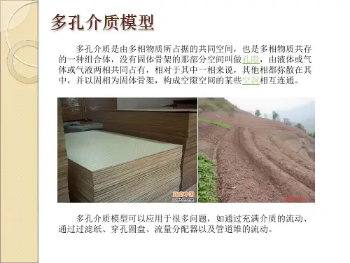
FLUENT帮助里自带的多孔介质算例-经典资料
- 格式:doc
- 大小:668.00 KB
- 文档页数:16
fluent多孔介质孔隙率FLUENT多孔介质是一个非常有用的数值模拟工具,因为它可以模拟各种多孔介质的过程。
其中,孔隙率是一个非常重要的参数,因为它可以影响多孔介质的物理和化学性质以及与周围环境的相互作用。
在本文中,我们将探讨FLUENT多孔介质中的孔隙率参数,帮助您更好地理解与其相关的内容。
步骤1:什么是孔隙率?孔隙率是指一个多孔介质中孔隙的总体积与样品总体积的比值。
可以用以下公式表示:φ = Vp / Vt × 100%其中,φ表示孔隙率,Vp表示孔隙的总体积,Vt表示样品的总体积。
步骤2:FLUENT多孔介质中的孔隙率参数在FLUENT中,我们可以使用两种方式来设置孔隙率参数:松散介质模型和实体多孔介质模型。
松散介质模型是一种将多孔介质视为连续介质的模型,其中孔隙率可以通过设置固体和流体的体积分数来确定。
在这种模型中,流体和固体的性质可以根据材料库选择或手动输入来确定。
实体多孔介质模型是一种将真实多孔介质视为离散孔隙和固体组成的模型。
在这种模型中,我们可以通过设置多孔介质的几何形状和孔隙率来模拟多孔介质的过程。
如果知道多孔介质的孔隙率,则可以手动输入。
如果不知道孔隙率,则可以使用体积渗透率来计算它。
步骤3:FLUENT多孔介质模拟中的应用FLUENT多孔介质模拟可以应用于许多领域,如环境保护,油藏开发,地下水资源管理等。
例如,在地下水资源管理中,孔隙率是一个非常重要的参数,因为它可以反映地下水含量和通透性。
使用FLUENT 多孔介质模拟可以确定地下水流量和渗透性,从而更好地管理我们的水资源。
类似的,FLUENT多孔介质也可以在油藏开发中估计原油储藏量和溢油模拟中模拟油污运移等。
总结FLUENT多孔介质模拟是一种非常强大的工具,可以帮助我们更好地理解多孔介质的物理和化学性质,以及与周围环境的相互作用。
孔隙率作为这个模拟过程中的一个重要参数,可以影响多孔介质的特性和FLUENT多孔介质模拟的精度。
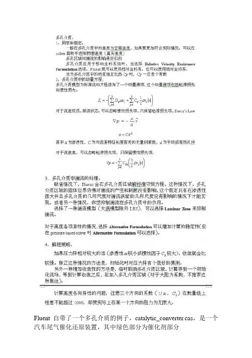
Fluent自带了一个多孔介质的例子,catalytic_converter.cas,是一个汽车尾气催化还原装置,其中绿色部分为催化剂部分其他设置就不说了,只说说与多孔介质有关的设置。
在建立模型时,必须将多孔介质单独划分为一个区域,然后才可以在设置边界条件时将这个区域设置为多孔介质。
1、在zone中选中该区域,在type中选中fluid,点set来到设置面板。
2、在Fluid面板中,选中Porous zone选项,如果忽略多孔区域对湍流的影响,选中Laminar zone。
3、首先是速度方向的设置,在2d中,在direction-1 vector中填入速度方向,在3d中,在direction-1 vector和direction-2 vector中填入速度方向,余下的未填方向,可以根据principal axis得到。
另外也可以用Update From Plane Tool来得到这两个量。
4、填入粘性阻力系数和惯性阻力系数,这两个系数可以通过经验公式得到。
在catalytic_converter.cas中可以看到x方向的阻力系数都比其他两个方向的阻力系数小1000倍,说明x方向是主要的压力降方向,其他两个方向不流通,压力降无限大。
(经验公式可以看帮助文件,其中有详细的介绍)。
随后的Power Law Model 中两个系数是另一种描述压力降的经验模型,一般不使用,可以保留缺省值0。
5、最后是Fluid Porosity,这个值只在模型选择了Physical Velocity 时才起作用,一般对计算没有影响,这个值要小于1。
补充:这个值在计算热传导时也起作用。
下面是改变一些参数后的比较。
1、速度方向的改变:原case:1、0、0 和0、1、0 y=0截面的速度矢量图修正case:-0.7366537、0.06852359、0.6727893 和0.6694272、-0.06727878、0.7398248 y=0速度矢量图2、修改Porosity值为0.5 原case,y=0截面修正case,y=0截面:修正case,且打开solver面板中的Physical Velocity选项:最后比较一下有多孔介质和无多孔介质对流场的影响。
ANSYS Fluent多孔介质模型简介
多孔介质是指内部含有众多空隙的固体材料,如土壤、煤炭、木材、过滤器、催化床等。
若采用详细的模型结构及网格划分处理,则会因为过多的网格数目而使计算量非常大,不能满足工程上的实际需求,而多孔介质模型实质上是将多孔介质区域结合了以经验假设为主的流动阻力,即动量源项。
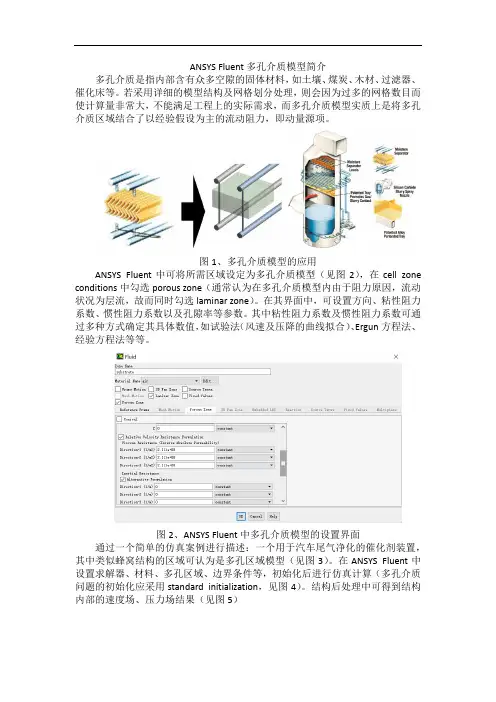
图1、多孔介质模型的应用
ANSYS Fluent中可将所需区域设定为多孔介质模型(见图2),在cell zone conditions中勾选porous zone(通常认为在多孔介质模型内由于阻力原因,流动状况为层流,故而同时勾选laminar zone)。
在其界面中,可设置方向、粘性阻力系数、惯性阻力系数以及孔隙率等参数。
其中粘性阻力系数及惯性阻力系数可通过多种方式确定其具体数值,如试验法(风速及压降的曲线拟合)、Ergun方程法、经验方程法等等。
图2、ANSYS Fluent中多孔介质模型的设置界面通过一个简单的仿真案例进行描述:一个用于汽车尾气净化的催化剂装置,其中类似蜂窝结构的区域可认为是多孔区域模型(见图3)。
在ANSYS Fluent中设置求解器、材料、多孔区域、边界条件等,初始化后进行仿真计算(多孔介质问题的初始化应采用standard initialization,见图4)。
结构后处理中可得到结构内部的速度场、压力场结果(见图5)
图3、汽车尾气净化器流动仿真
图4、ANSYS Fluent初始化界面
图5、不同截面的速度场云图、压力场云图及压力曲线。
Fluent自带了一个多孔介质的例子,catalytic_converter.cas,是一个汽车尾气催化还原装置,其中绿色部分为催化剂部分其他设置就不说了,只说说与多孔介质有关的设置。
在建立模型时,必须将多孔介质单独划分为一个区域,然后才可以在设置边界条件时将这个区域设置为多孔介质。
1、在zone中选中该区域,在type中选中fluid,点set来到设置面板。
2、在Fluid面板中,选中Porous zone选项,如果忽略多孔区域对湍流的影响,选中Laminar zone。
3、首先是速度方向的设置,在2d中,在direction-1 vector中填入速度方向,在3d中,在direction-1 vector和direction-2 vector中填入速度方向,余下的未填方向,可以根据principal axis得到。
另外也可以用Update From Plane Tool来得到这两个量。
4、填入粘性阻力系数和惯性阻力系数,这两个系数可以通过经验公式得到。
在catalytic_converter.cas中可以看到x方向的阻力系数都比其他两个方向的阻力系数小1000倍,说明x方向是主要的压力降方向,其他两个方向不流通,压力降无限大。
(经验公式可以看帮助文件,其中有详细的介绍)。
随后的Power Law Model 中两个系数是另一种描述压力降的经验模型,一般不使用,可以保留缺省值0。
5、最后是Fluid Porosity,这个值只在模型选择了Physical Velocity 时才起作用,一般对计算没有影响,这个值要小于1。
补充:这个值在计算热传导时也起作用。
下面是改变一些参数后的比较。
1、速度方向的改变:原case:1、0、0 和0、1、0 y=0截面的速度矢量图修正case:-0.7366537、0.06852359、0.6727893 和0.6694272、-0.06727878、0.7398248 y=0速度矢量图2、修改Porosity值为0.5 原case,y=0截面修正case,y=0截面:修正case,且打开solver面板中的Physical Velocity选项:最后比较一下有多孔介质和无多孔介质对流场的影响。
多孔介质系数的计算方法1.STAR-CCM+中的多孔介质系数(文中所述的Excel文档以及模型源文件均可通过文中图片获取下载地址)在STAR-CCM+中主要需要设置多孔惯性阻力、多孔粘性阻力、孔隙率等参数。
孔隙率为流体在多孔介质中所占的分数,由标量分布法指定,取值介于0-1之间。
通过多孔介质的流量可根据达西定律描述,它基于渗透力度量以使流速与压力梯度相关联。
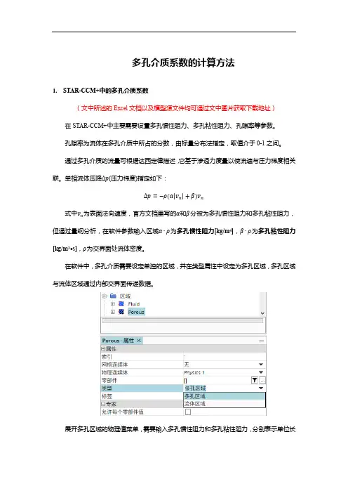
单相流体压降Δp(压力梯度)指定如下:Δp=−ρ(α|v n|+β)v n式中v n为表面法向速度,官方文档里写的α和β分被为多孔惯性阻力和多孔粘性阻力,但通过量纲分析,在软件参数输入区域α∙ρ为多孔惯性阻力[kg/m4],β∙ρ为多孔粘性阻力[kg/m3·s],ρ为交界面处流体密度。
在软件中,多孔介质需要设定单独的区域,并在类型属性中设定为多孔区域,多孔区域与流体区域通过内部交界面传递数据。
展开多孔区域的物理值菜单,需要输入多孔惯性阻力和多孔粘性阻力,分别表示单位长度的惯性量和粘性量值。
下图以正交各项异性参数为例展示需要输入参数的位置。
多孔惯性阻力和多孔粘性阻力的值通过试验数据的拟合求得,以散热器为例,对散热器芯体进行单体性能试验,得到所通过的气体(密度为1.18415kg/m3)流量和总压降的关系,转化为速度和总压降的关系如下所示。
在Excel中对数据进行拟合,将总压力转换为压力梯度,通过计算可得多孔惯性阻力和多孔粘性阻力。
得到的多孔惯性阻力和多孔粘性阻力是沿流动方向的阻力系数,另外两个方向通常取为比主流方向阻力系数大2-3个数量级的值,以阻止流体在这两个方向上的流动,但取值过大可能会影响收敛性。
下图为计算的Excel文件,填入试验数据即可得两个阻力系数。
下载本文档,将扩展名docx改为rar,得到一个压缩包文件,双击打开,再依次打开word、media文件夹。
然后将media文件夹下的image4.jpg拖拽至桌面或某个文件夹,将其扩展名jpg改为rar,解压缩可得一个包含模型和Excel文件下载地址的txt文本文档download.txt。
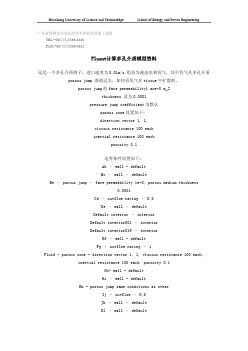
广东省深圳市宝安区沙井辛养社区西部工业园 TEL:+86-755-3366-8888 FAX:+86-755-3366-0612Fluent计算多孔介质模型资料这是一个多孔介质例子,进口速度为0.01m/s,组份为液态水和氧气,其中氧气从多孔介质porous jump 渗透过去,如何看氧气在tissue中扩散的。
porous jump的face permeability1 a=e-8 m_2thickness 设为0.0001pressure jump coefficient为默认porous zone设置如下:direction vector 1, 1,viscous resistance 100 eachinertial resistance 100 eachporosity 0.1边界条件设置如下:Ab – wall - defaultBc – wall – defaultBe – porous jump – face permeability 1e-8, porous medium thickness0.0001Cd – outflow rating – 0.5De – wall – defaultDefault interior – interiorDefault interior001 – interiorDefault interior019 – interiorEf – wall - defaultFg – outflow rating – 1Fluid - porous zone - direction vector 1, 1, viscous resistance 100 each,inertial resistance 100 each, porosity 0.1Gh- wall - defaultHi – wall - defaultHk - porous jump same conditions as otherIj – outflow – 0.5Jk – wall – defaultKl – wall – defaultLa – velocity inlet – 0.01 m/s, temperature 300K, 0.5 mass fraction O2 Lfluid – porous zone - direction vector 1, 1, viscous resistance 100 each,inertial resistance 100 each, porosity 0.1Pipefluid – fluid – default (no porous zone)Models – species transport – water and oxygen mixtureVariations – different boundary conditions at top and bottom (outflow, wall ect)注意,其中porous zone在gambit中设置为fluid,在fluent中设置为porous zone边界条件设置如下:Ab – wall - defaultBc – wall – defaultBe – porous jump – face permeability 1e-8, porous medium thickness0.0001Cd – outflow rating – 0.5De – wall – defaultDefault interior – interiorDefault interior001 – interiorDefault interior019 – interiorEf – wall - defaultFg – outflow rating – 1Fluid - porous zone - direction vector 1, 1, viscous resistance 100 each,inertial resistance 100 each, porosity 0.1Gh- wall - defaultHi – wall - defaultHk - porous jump same conditions as otherIj – outflow – 0.5Jk – wall – defaultKl – wall – defaultLa – velocity inlet – 0.01 m/s, temperature 300K, 0.5 mass fraction O2 Lfluid – porous zone - direction vector 1, 1, viscous resistance 100 each,inertial resistance 100 each, porosity 0.1Pipefluid – fluid – default (no porous zone)Models – species transport – water and oxygen mixtureVariations – different boundary conditions at top and bottom (outflow, wall ect) 注意,其中porous zone在gambit中设置为fluid,在fluent中设置为porous zone。
fluent 多孔介质厄根公式Fluent多孔介质厄根公式是描述流体在多孔介质中流动行为的重要公式之一。
它是由荷兰物理学家Darcy和德国物理学家厄根分别在19世纪中叶和20世纪初提出的,被广泛应用于地下水、石油开采、土壤水分运动等领域的研究和工程实践中。
Fluent多孔介质厄根公式的基本形式为:u = -K(∇P)/μ其中,u代表流体的平均流速,K代表多孔介质的渗透率,∇P代表压力梯度,μ代表流体的动力粘度。
多孔介质厄根公式的推导基于一系列假设和简化。
首先,假设多孔介质是均匀各向同性的,即渗透率在空间上是均匀分布的;其次,假设流体是层流流动,即流体的速度分布是稳定的;最后,假设流体的粘度是恒定的,即不随流速和温度的变化而变化。
根据多孔介质厄根公式,流速u与压力梯度∇P成正比,与渗透率K 成反比,与流体的动力粘度μ成正比。
这意味着,在相同的压力梯度下,流速与渗透率呈反比关系,即渗透率越大,流速越小;而在相同的渗透率下,流速与流体的动力粘度成正比,即流体的粘度越大,流速越小。
多孔介质厄根公式的应用范围广泛。
在地下水领域,它被用来描述地下水的流动行为,如地下水的渗流速度、地下水的排泄量等。
在石油开采领域,它被用来研究油藏中原油的渗流行为,如原油的采收率、油井的产能等。
在土壤水分运动领域,它被用来分析土壤中水分的流动规律,如土壤中水分的运移速率、土壤的水分保持能力等。
然而,多孔介质厄根公式也有其局限性。
首先,它基于一系列的假设和简化,因此只适用于特定条件下的流动问题。
其次,它忽略了多孔介质中的微观结构和孔隙分布的影响,因此在非均匀介质和复杂多孔介质中的应用存在一定的误差。
为了更准确地描述多孔介质中的流动行为,研究者们提出了一系列改进和扩展的模型和方法。
例如,根据多孔介质的孔隙结构和流体的物理性质,可以建立更精细的渗透率模型;利用数值模拟方法,可以模拟多孔介质中复杂的流动过程;通过实验和观测,可以获取更准确的渗透率和流速数据。
多孔介质条件多孔介质模型可以应用于很多问题,如通过充满介质的流动、通过过滤纸、穿孔圆盘、流量分配器以及管道堆的流动。
当你使用这一模型时,你就定义了一个具有多孔介质的单元区域,而且流动的压力损失由多孔介质的动量方程中所输入的内容来决定。
通过介质的热传导问题也可以得到描述,它服从介质和流体流动之间的热平衡假设,具体内容可以参考多孔介质中能量方程的处理一节。
多孔介质的一维化简模型,被称为多孔跳跃,可用于模拟具有已知速度/压降特征的薄膜。
多孔跳跃模型应用于表面区域而不是单元区域,并且在尽可能的情况下被使用(而不是完全的多孔介质模型),这是因为它具有更好的鲁棒性,并具有更好的收敛性。
详细内容请参阅多孔跳跃边界条件。
1、多孔介质模型的限制如下面各节所述,多孔介质模型结合模型区域所具有的阻力的经验公式被定义为“多孔”。
事实上多孔介质不过是在动量方程中具有了附加的动量损失而已。
因此,下面模型的限制就可以很容易的理解了。
● 流体通过介质时不会加速,因为事实上出现的体积的阻塞并没有在模型中出现。
这对于过渡流是有很大的影响的,因为它意味着FLUENT 不会正确的描述通过介质的过渡时间。
● 多孔介质对于湍流的影响只是近似的。
详细内容可以参阅湍流多孔介质的处理一节。
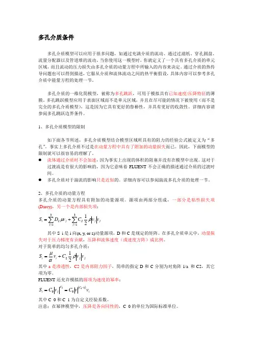
2、多孔介质的动量方程多孔介质的动量方程具有附加的动量源项。
源项由两部分组成,一部分是粘性损失项 (Darcy),另一个是内部损失项:∑∑==+=313121j j j j ijj ij i v v C v D S ρμ 其中S_i 是i 向(x, y, or z)动量源项,D 和C 是规定的矩阵。
在多孔介质单元中,动量损失对于压力梯度有贡献,压降和流体速度(或速度方阵)成比例。
对于简单的均匀多孔介质:j j i i v v C v S ραμ212+= 其中a 是渗透性,C2是内部阻力因子,简单的指定D 和C 分别为对角阵1/a 和C2,其它项为零。
FLUENT 还允许模拟的源项为速度的幂率:()i C C j i v v C v C S 10011-==其中C_0和C_1为自定义经验系数。
FLUENT多孔介质数值模拟设置C=对于不同D/t的不同雷诺数范围被列成不同的表的系数A_p=圆盘的面积(固体和洞)如果你选择在多孔介质中模拟热传导,你必须指定多孔介质中的材料以及多孔性。
要定义多孔介质的材料,向下拉流体面板中阻力输入底下的滚动条,然后在多孔热传导的固体材料下拉列表中选中适当的固体。
另一个处理收敛性差的要领是临时取消多孔介质模型(在流体面板中关闭多孔区域)然后获取一个不受多孔区域影响的初始流场。
取消多孔区域后,FLUENT会将多孔区域处理为流体区域并按响应的流体区域来计算。
一旦获取了初始解,或者计算很容易收敛,你就可以激活多孔模型继续计算包罗多孔区域的流场(对于大阻力多孔介质不保举使用该要领)。
这些变量会在后处理面板的变量选择下拉菜谱制定类别中出现。
然后在多孔热传导下设定多孔性。
多孔性f是多孔介质中流体的体积分数(即介质的开放体积分数)。
多孔性用于介质中的热传导预测,处理要领请参阅多孔介质能量方程的处理一节。
它还对介质中的反应源项和体力的计算有影响。
这个源项和介质中流体的体积成比例。
如果你想要模拟完全开放的介质(固体介质没有影响),你应该设定多孔性为1.0。
当多孔性为1.0时,介质的固体部门对于热传导和(或)热源项/反应源项没有影响。
注意:多孔性永远不会影响介质中的流体速率,这已经在多孔介质的动量方程一节中介绍了。
不管你将多孔性设定为何值,,FLUENT所预测的速率都是介质中的外貌速率。
对于多孔介质动量源项(多孔介质动量方程中的方程5),如果你使用幂律模型近似,你只要在流体面板的幂律模型中输入系数C_0和C_1就可以了。
如果C_0或C_1为非零值,解算器会忽略面板中除了多孔介质幂律模型之外的所有输入。
定义源项一般说来,在模拟多孔介质时,你可以使用标准的解算步骤以及解参数的设置。
然而你会发现如果多孔区域在流动方向上压降至关大(比如:渗透性a很低或者内部因数C_2很大)的话,解的收敛速率就会变慢。
FLUENT多孔介质数值模拟设置多孔介质条件多孔介质模型可以应用于很多问题,如通过充满介质的流动、通过过滤纸、穿孔圆盘、流量分配器以及管道堆的流动。
当你使用这一模型时,你就定义了一个具有多孔介质的单元区域,而且流动的压力损失由多孔介质的动量方程中所输入的内容来决定。
通过介质的热传导问题也可以得到描述,它服从介质和流体流动之间的热平衡假设,具体内容可以参考多孔介质中能量方程的处理一节。
多孔介质的一维化简模型,被称为多孔跳跃,可用于模拟具有已知速度/压降特征的薄膜。
多孔跳跃模型应用于表面区域而不是单元区域,并且在尽可能的情况下被使用(而不是完全的多孔介质模型),这是因为它具有更好的鲁棒性,并具有更好的收敛性。
详细内容请参阅多孔跳跃边界条件。
多孔介质模型的限制如下面各节所述,多孔介质模型结合模型区域所具有的阻力的经验公式被定义为“多孔”。
事实上多孔介质不过是在动量方程中具有了附加的动量损失而已。
因此,下面模型的限制就可以很容易的理解了。
流体通过介质时不会加速,因为事实上出现的体积的阻塞并没有在模型中出现。
这对于过渡流是有很大的影响的,因为它意味着FLUENT不会正确的描述通过介质的过渡时间。
多孔介质对于湍流的影响只是近似的。
详细内容可以参阅湍流多孔介质的处理一节。
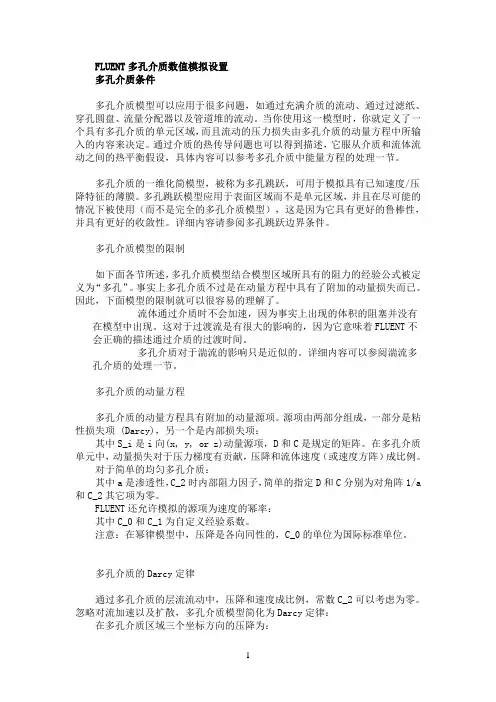
多孔介质的动量方程多孔介质的动量方程具有附加的动量源项。
源项由两部分组成,一部分是粘性损失项 (Darcy),另一个是内部损失项:其中S_i是i向(x, y, or z)动量源项,D和C是规定的矩阵。
在多孔介质单元中,动量损失对于压力梯度有贡献,压降和流体速度(或速度方阵)成比例。
对于简单的均匀多孔介质:其中a是渗透性,C_2时内部阻力因子,简单的指定D和C分别为对角阵1/a 和C_2其它项为零。
FLUENT还允许模拟的源项为速度的幂率:其中C_0和C_1为自定义经验系数。
注意:在幂律模型中,压降是各向同性的,C_0的单位为国际标准单位。
多孔介质的Darcy定律通过多孔介质的层流流动中,压降和速度成比例,常数C_2可以考虑为零。
(整理)多孔介质-Fluent模拟7.19多孔介质边界条件多孔介质模型适用的范围非常广泛,包括填充床,过滤纸,多孔板,流量分配器,还有管群,管束系统。
当使用这个模型的时候,多孔介质将运用于网格区域,流场中的压降将由输入的条件有关,见Section 7.19.2.同样也可以计算热传导,基于介质和流场热量守恒的假设,见Section 7.19.3.通过一个薄膜后的已知速度/压力降低特性可以简化为一维多孔介质模型,简称为“多孔跳跃”。
多孔跳跃模型被运用于一个面区域而不是网格区域,而且也可以代替完全多孔介质模型在任何可能的时候,因为它更加稳定而且能够很好地收敛。
见Section 7.22.7.19.1 多孔介质模型的限制和假设多孔介质模型就是在定义为多孔介质的区域结合了一个根据经验假设为主的流动阻力。
本质上,多孔介质模型仅仅是在动量方程上叠加了一个动量源项。
这种情况下,以下模型方面的假设和限制就可以很容易得到:因为没有表示多孔介质区域的实际存在的体,所以fluent默认是计算基于连续性方程的虚假速度。
做为一个做精确的选项,你可以适用fluent中的真是速度,见section7.19.7。
多孔介质对湍流流场的影响,是近似的,见7.19.4。
当在移动坐标系中使用多孔介质模型的时候,fluent既有相对坐标系也可以使用绝对坐标系,当激活相对速度阻力方程。
这将得到更精确的源项。
相关信息见section7.19.5和7.19.6。
当需要定义比热容的时候,必须是常数。
7.19.2 多孔介质模型动量方程多孔介质模型的动量方程是在标准动量方程的后面加上动量方程源项。
源项包含两个部分:粘性损失项(达西公式项,方程7.19-1右边第一项),和惯性损失项(方程7.19-1右边第二项)(7.19-1)式中,si是i(x,y,z)动量方程的源项,是速度大小,D和C 是矩阵。
动量源项对多孔介质区域的压力梯度有影响,生成一个与速度大小(速度平方)成正比的压降。
7.19多孔介质边界条件多孔介质模型适用的范围非常广泛,包括填充床,过滤纸,多孔板,流量分配器,还有管群,管束系统。
当使用这个模型的时候,多孔介质将运用于网格区域,流场中的压降将由输入的条件有关,见Section 7.19.2.同样也可以计算热传导,基于介质和流场热量守恒的假设,见Section 7.19.3.通过一个薄膜后的已知速度/压力降低特性可以简化为一维多孔介质模型,简称为“多孔跳跃”。
多孔跳跃模型被运用于一个面区域而不是网格区域,而且也可以代替完全多孔介质模型在任何可能的时候,因为它更加稳定而且能够很好地收敛。
见Section 7.22.7.19.1 多孔介质模型的限制和假设多孔介质模型就是在定义为多孔介质的区域结合了一个根据经验假设为主的流动阻力。
本质上,多孔介质模型仅仅是在动量方程上叠加了一个动量源项。
这种情况下,以下模型方面的假设和限制就可以很容易得到:•因为没有表示多孔介质区域的实际存在的体,所以fluent默认是计算基于连续性方程的虚假速度。
做为一个做精确的选项,你可以适用fluent中的真是速度,见section7.19.7。
•多孔介质对湍流流场的影响,是近似的,见7.19.4。
•当在移动坐标系中使用多孔介质模型的时候,fluent既有相对坐标系也可以使用绝对坐标系,当激活相对速度阻力方程。
这将得到更精确的源项。
相关信息见section7.19.5和7.19.6。
•当需要定义比热容的时候,必须是常数。
7.19.2 多孔介质模型动量方程多孔介质模型的动量方程是在标准动量方程的后面加上动量方程源项。
源项包含两个部分:粘性损失项(达西公式项,方程7.19-1右边第一项),和惯性损失项(方程7.19-1右边第二项)(7.19-1)式中,si是i(x,y,z)动量方程的源项,是速度大小,D和C是矩阵。
动量源项对多孔介质区域的压力梯度有影响,生成一个与速度大小(速度平方)成正比的压降。
经过痛苦的一段经历,终于将局部问题真相大白,为了使保位同仁不再经过我之痛苦,现在将本人多孔介质经验公布如下,希望各位能加精:1。
Gambit 中划分网格之后,定义需要做为多孔介质的区域为fluid, 与缺省的fluid 分别开来,再定义其名称,我习惯将名称定义为porous;2。
在fluent 中定义边界条件define-boundary condition-porous(刚定义的名称),将其设置边界条件为fluid, 点击set 按钮即弹出与fluid 边界条件一样的对话框,选中porous zone 与laminar 复选框, 再点击porous zone 标签即出现一个带有滚动条的界面;3。
porous zone 设置方法:1)定义矢量:二维定义一个矢量,第二个矢量方向不用定义,是与第一个矢量方向正交的;三维定义二个矢量,第三个矢量方向不用定义,是与第一、二个矢量方向正交的;(如何知道矢量的方向:打开grid 图,看看X,Y,Z 的方向,如果是X 向,矢量为1,0,0, 同理Y 向为0,1,0 ,Z 向为0,0,1, 如果所需要的方向与坐标轴正向相反,则定义矢量为负)圆锥坐标与球坐标请参考fluent 帮助。
2)定义粘性阻力1/a 与内部阻力C2:请参看本人上一篇博文“ 终于搞清fluent 中多孔粘性阻力与内部阻力的计算方法”,此处不赘述;3)如果了定义粘性阻力1/a 与内部阻力C2,就不用定义C1 与C0,因为这是两种不同的定义方法,C1与C0 只在幂率模型中出现,该处保持默认就行了;4)定义孔隙率porousity ,默认值1 表示全开放,此值按实验测值填写即可。
完了,其他设置与普通k-e 或RSM相同。
总结一下,与君共享!Tutorial 7. Modeling Flow Through Porous MediaIntroductionMany industrial applications involve the modeling of flow through porous media, such as filters, catalyst beds, and packing. This tutorial illustrates how to set up and solve a problem involving gas flow through porous media.The industrial problem solved here involves gas flow through a catalytic converter. Catalytic converters are commonly used to purify emissions from gasoline and diesel engines by converting environmentally hazardous exhaust emissions to acceptable substances.Examples of such emissions include carbon monoxide (CO), nitrogen oxides (NOx), and unburned hydrocarbon fuels. These exhaust gas emissions are forced through a substrate, which is a ceramic structure coated with a metal catalyst such as platinum or palladium.The nature of the exhaust gas flow is a very important factor in determining the performance of the catalytic converter. Of particular importance is the pressure gradient and velocity distribution through the substrate. Hence CFD analysis is used to design efficient catalytic converters: by modeling the exhaust gas flow, the pressure drop and the uniformity of flow through the substrate can be determined. In this tutorial, FLUENT is used to model the flow of nitrogen gas through a catalytic converter geometry, so that the flow field structure may be analyzed.This tutorial demonstrates how to do the following:_ Set up a porous zone for the substrate with appropriate resistances._ Calculate a solution for gas flow through the catalytic converter using the pressure based solver._ Plot pressure and velocity distribution on specified planes of the geometry._ Determine the pressure drop through the substrate and the degree of non-uniformity of flow through cross sections of the geometry using X-Y plots and numerical reports.Problem DescriptionThe catalytic converter modeled here is shown in Figure 7.1. The nitrogen flows in through the inlet with a uniform velocity of 22.6 m/s, passes through a ceramic monolith substrate with square shaped channels, and then exits through the outlet.While the flow in the inlet and outlet sections is turbulent, the flow through the substrate is laminar and is characterized by inertial and viscous loss coefficients in the flow (X) direction. The substrate is impermeable in other directions, which is modeled using loss coefficients whose values are three orders of magnitude higher than in the X direction.Setup and SolutionStep 1: Grid1. Read the mesh file (catalytic converter.msh).File /Read /Case...2. Check the grid. Grid /CheckFLUENT will perform various checks on the mesh and report the progress in the console. Make sure that the minimum volume reported is a positive number.3. Scale the grid.Grid! Scale...(a) Select mm from the Grid Was Created In drop-down list.(b) Click the Change Length Units button. All dimensions will now be shown in millimeters.(c) Click Scale and close the Scale Grid panel.4. Display the mesh. Display /Grid...(a) Make sure that inlet, outlet, substrate-wall, and wall are selected in the Surfaces selection list.(b) Click Display.(c) Rotate the view and zoom in to get the display shown in Figure 7.2.(d) Close the Grid Display panel.The hex mesh on the geometry contains a total of 34,580 cells.Step 2: Models1. Retain the default solver settings. Define /Models /Solver...2. Select the standard k-ε turbulence model. Define/ Models /Viscous...Step 3: Materials1. Add nitrogen to the list of fluid materials by copying it from the Fluent Database for materials. Define /Materials...(a)Click the Fluent Database... button to open the Fluent Database Materials panel.(a) Select nitrogen from the Material Name drop-down list.(b)Click OK to close the Fluid panel.2. Set the boundary conditions for the substrate (substrate).i. Select nitrogen (n2) from the list of Fluent Fluid Materials.ii. Click Copy to copy the information for nitrogen to your list of fluid materials. iii. Close the Fluent Database Materials panel. (b) Close the Materials panel. Step 4: Boundary Conditions.1. Set the boundary conditions for the fluid (fluid).Define /Boundary Conditions...(a) Select nitrogen from the Material Name drop-down list.(b) Enable the Porous Zone option to activate the porous zone model.(c) Enable the Laminar Zone option to solve the flow in the porous zone without turbulence.(d) Click the Porous Zone tab.i. Make sure that the principal direction vectors are set as shown in Table7.1. Use the scroll bar to access the fields that are not initially visible in the panel.ii. Enter the values in Table 7.2 for the Viscous Resistance and Inertial Resistance. Scroll down to access the fields that are not initially visible in the panel.(e) Click OK to close the Fluid panel.3. Set the velocity and turbulence boundary conditions at the inlet (inlet).(a) Enter 22.6 m/s for the Velocity Magnitude.(b) Select Intensity and Hydraulic Diameter from the Specification Method dropdown list in the Turbulence group box.(c) Retain the default value of 10% for the Turbulent Intensity.(d) Enter 42 mm for the Hydraulic Diameter.(e) Click OK to close the Velocity Inlet panel.4. Set the boundary conditions at the outlet (outlet).(a) Retain the default setting of 0 for Gauge Pressure.(b) Select Intensity and Hydraulic Diameter from the Specification Method dropdown list in the Turbulence group box.(c) Enter 5% for the Backflow Turbulent Intensity.(d) Enter 42 mm for the Backflow Hydraulic Diameter.(e) Click OK to close the Pressure Outlet panel.5. Retain the default boundary conditions for the walls (substrate-wall and wall) and close the Boundary Conditions panel.Step 5: Solution1. Set the solution parameters. Solve /Controls /Solution...(a) Retain the default settings for Under-Relaxation Factors.(b) Select Second Order Upwind from the Momentum drop-down list in the Discretization group box.(c) Click OK to close the Solution Controls panel.2. Enable the plotting of residuals during the calculation. Solve/Monitors /Residual...(a)Enable Plot in the Options group box.(b)Click OK to close the Residual Monitors panel.3.Enable the plotting of the mass flow rate at the outlet.Solve / Monitors /Surface...(a) Set the Surface Monitors to 1.(b) Enable the Plot and Write options for monitor-1, and click the Define... button to open the Define Surface Monitor panel.i. Select Mass Flow Rate from the Report Type drop-down list.ii. Select outlet from the Surfaces selection list.iii. Click OK to close the Define Surface Monitors panel.(c) Click OK to close the Surface Monitors panel.4. Initialize the solution from the inlet. Solve /Initialize /Initialize...(a) Select inlet from the Compute From drop-down list.(b) Click Init and close the Solution Initialization panel.5. Save the case file (catalytic converter.cas). File /Write /Case...6. Run the calculation by requesting 100 iterations. Solve /Iterate...(a) Enter 100 for the Number of Iterations.(b) Click Iterate.The FLUENT calculation will converge in approximately 70 iterations. By this point the mass flow rate monitor has attended out, as seen in Figure 7.3.(c) Close the Iterate panel.7. Save the case and data files (catalytic converter.cas and catalytic converter.dat). File /Write /Case & Data...Note: If you choose a file name that already exists in the current folder, FLUENT will prompt you for confirmation to overwrite the file.Step 6: Post-processing1. Create a surface passing through the centerline for post-processing purposes.Surface/Iso-Surface...(a) Select Grid... and Y-Coordinate from the Surface of Constant drop-down lists.(b) Click Compute to calculate the Min and Max values.(c) Retain the default value of 0 for the Iso-Values.(d) Enter y=0 for the New Surface Name.(e) Click Create.2. Create cross-sectional surfaces at locations on either side of the substrate, as well as at its center.Surface /Iso-Surface...(a) Select Grid... and X-Coordinate from the Surface of Constant drop-down lists.(b) Click Compute to calculate the Min and Max values.(c) Enter 95 for Iso-Values.(d) Enter x=95 for the New Surface Name.(e) Click Create.(f) In a similar manner, create surfaces named x=130 and x=165 with Iso-Values of 130 and 165, respectively. Close the Iso-Surface panel after all the surfaces have been created.3. Create a line surface for the centerline of the porous media.Surface /Line/Rake...(a) Enter the coordinates of the line under End Points, using the starting coordinate of (95, 0, 0) and an ending coordinate of (165, 0, 0), as shown.(b) Enter porous-cl for the New Surface Name.(c) Click Create to create the surface.(d) Close the Line/Rake Surface panel.4. Display the two wall zones (substrate-wall and wall). Display /Grid...(a) Disable the Edges option.(b) Enable the Faces option.(c) Deselect inlet and outlet in the list under Surfaces, and make sure that only substrate-wall and wall are selected.(d) Click Display and close the Grid Display panel.(e) Rotate the view and zoom so that the display is similar to Figure 7.2.5. Set the lighting for the display. Display /Options...(a) Enable the Lights On option in the Lighting Attributes group box.(b) Retain the default selection of Gourand in the Lighting drop-down list.(c) Click Apply and close the Display Options panel.6. Set the transparency parameter for the wall zones (substrate-wall and wall). Display/Scene...(a) Select substrate-wall and wall in the Names selection list.(b) Click the Display... button under Geometry Attributes to open the Display Properties panel.i. Set the Transparency slider to 70.ii. Click Apply and close the Display Properties panel.(c) Click Apply and then close the Scene Description panel.7. Display velocity vectors on the y=0 surface.Display /Vectors...(a) Enable the Draw Grid option. The Grid Display panel will open.i. Make sure that substrate-wall and wall are selected in the list under Surfaces.ii. Click Display and close the Display Grid panel.(b) Enter 5 for the Scale.(c) Set Skip to 1.(d) Select y=0 from the Surfaces selection list.(e) Click Display and close the Vectors panel.The flow pattern shows that the flow enters the catalytic converter as a jet, with recirculation on either side of the jet. As it passes through the porous substrate, it decelerates and straightens out, and exhibits a more uniform velocity distribution.This allows the metal catalyst present in the substrate to be more effective.Figure 7.4: Velocity Vectors on the y=0 Plane8. Display filled contours of static pressure on the y=0 plane.Display /Contours...(a) Enable the Filled option.(b) Enable the Draw Grid option to open the Display Grid panel.i. Make sure that substrate-wall and wall are selected in the list under Surfaces.ii. Click Display and close the Display Grid panel.(c) Make sure that Pressure... and Static Pressure are selected from the Contours of drop-down lists.(d) Select y=0 from the Surfaces selection list.(e) Click Display and close the Contours panel.Figure 7.5: Contours of the Static Pressure on the y=0 planeThe pressure changes rapidly in the middle section, where the fluid velocity changes as it passes through the porous substrate. The pressure drop can be high, due to the inertial and viscous resistance of the porous media. Determining this pressure drop is a goal of CFD analysis. In the next step, you will learn how to plot the pressure drop along the centerline of the substrate.9. Plot the static pressure across the line surface porous-cl.Display /Contours...Plot /XY Plot...(a) Make sure that the Pressure... and Static Pressure are selected from the Y Axis Function drop-down lists.(b) Select porous-cl from the Surfaces selection list.(c)Click Plot and close the Solution XY Plot panel.(a) Disable the Global Range option.Figure 7.6: Plot of the Static Pressure on the porous-cl Line SurfaceIn Figure 7.6, the pressure drop across the porous substrate can be seen to be roughly 300 Pa.10. Display filled contours of the velocity in the X direction on the x=95, x=130 and x=165 surfaces.(b) Select Velocity... and X Velocity from the Contours of drop-down lists.(c) Select x=130, x=165, and x=95 from the Surfaces selection list, and deselect y=0.(d) Click Display and close the Contours panel.The velocity profile becomes more uniform as the fluid passes through the porous media. The velocity is very high at the center (the area in red) just before the nitrogen enters the substrate and then decreases as it passes through and exits the substrate. The area in green, which corresponds to a moderate velocity, increases in extent.Figure 7.7: Contours of the X Velocity on the x=95, x=130, and x=165 Surfaces 11. Use numerical reports to determine the average, minimum, and maximum of the velocity distribution before and after the porous substrate.Report /Surface Integrals...(a) Select Mass-Weighted Average from the Report Type drop-down list.(b) Select Velocity and X Velocity from the Field Variable drop-down lists.(c) Select x=165 and x=95 from the Surfaces selection list.(d) Click Compute.(e) Select Facet Minimum from the Report Type drop-down list and click Compute again.(f) Select Facet Maximum from the Report Type drop-down list and click Compute again.(g) Close the Surface Integrals panel.The numerical report of average, maximum and minimum velocity can be seen in the main FLUENT console, as shown in the following example:The spread between the average, maximum, and minimum values for X velocity gives the degree to which the velocity distribution is non-uniform. You can also use these numbers to calculate the velocity ratio (i.e., the maximum velocity divided by the mean velocity) and the space velocity (i.e., the product of the mean velocity and the substrate length).Custom field functions and UDFs can be also used to calculate more complex measures of non-uniformity, such as the standard deviation and the gamma uniformity index.SummaryIn this tutorial, you learned how to set up and solve a problem involving gas flow through porous media in FLUENT. You also learned how to perform appropriate post-processing to investigate the flow field, determine the pressure drop across the porous media and non-uniformity of the velocity distribution as the fluid goes through the porous media.Further ImprovementsThis tutorial guides you through the steps to reach an initial solution. You may be able to obtain a more accurate solution by using an appropriate higher-order discretization scheme and by adapting the grid. Grid adaption can also ensure that the solution is independent of the grid. These steps are demonstrated in Tutorial 1.。
Chapter 10: Modeling Flow Through Porous MediaThis tutorial is divided into the following sections:10.1. Introduction10.2. Prerequisites10.3. Problem Description10.4. Setup and Solution10.5. Summary10.6. Further Improvements10.1. IntroductionMany industrial applications such as filters, catalyst beds and packing, involve modeling the flow through porous media.This tutorial illustrates how to set up and solve a problem involving gas flow through porous media.The industrial problem solved here involves gas flow through a catalytic converter. Catalytic converters are commonly used to purify emissions from gasoline and diesel engines by converting environmentally hazardous exhaust emissions to acceptable substances. Examples of such emissions include carbon monoxide (CO), nitrogen oxides (NOx), and unburned hydrocarbon fuels.These exhaust gas emissionsare forced through a substrate, which is a ceramic structure coated with a metal catalyst such as platinum or palladium.The nature of the exhaust gas flow is a very important factor in determining the performance of the catalytic converter. Of particular importance is the pressure gradient and velocity distribution throughthe substrate. Hence CFD analysis is used to design efficient catalytic converters. By modeling the exhaust gas flow, the pressure drop and the uniformity of flow through the substrate can be determined. Inthis tutorial, ANSYS FLUENT is used to model the flow of nitrogen gas through a catalytic converter geometry, so that the flow field structure may be analyzed.This tutorial demonstrates how to do the following:•Set up a porous zone for the substrate with appropriate resistances.•Calculate a solution for gas flow through the catalytic converter using the pressure-based solver.•Plot pressure and velocity distribution on specified planes of the geometry.•Determine the pressure drop through the substrate and the degree of non-uniformity of flow through cross sections of the geometry using X-Y plots and numerical reports.10.2. PrerequisitesThis tutorial is written with the assumption that you have completed one or more of the introductory tutorials found in this manual:•Introduction to Using ANSYS FLUENT in ANSYS Workbench: Fluid Flow and Heat Transfer in a Mixing Elbow (p.1)•Parametric Analysis in ANSYS Workbench Using ANSYS FLUENT (p.77)Chapter 10: Modeling Flow Through Porous Media•Introduction to Using ANSYS FLUENT: Fluid Flow and Heat Transfer in a Mixing Elbow (p.131)and that you are familiar with the ANSYS FLUENT navigation pane and menu structure. Some steps in the setup and solution procedure will not be shown explicitly.10.3. Problem DescriptionThe catalytic converter modeled here is shown in Figure 10.1 (p.448).The nitrogen flows through the inlet with a uniform velocity of 22.6 m/s, passes through a ceramic monolith substrate with square-shaped channels, and then exits through the outlet.Figure 10.1 Catalytic Converter Geometry for Flow ModelingWhile the flow in the inlet and outlet sections is turbulent, the flow through the substrate is laminar and is characterized by inertial and viscous loss coefficients along the inlet axis.The substrate is imper-meable in other directions.This characteristic is modeled using loss coefficients that are three orders of magnitude higher than in the main flow direction.10.4. Setup and SolutionThe following sections describe the setup and solution steps for this tutorial:10.4.1. Preparation10.4.2. Step 1: Mesh10.4.3. Step 2: General Settings10.4.4. Step 3: Models10.4.5. Step 4: Materials10.4.6. Step 5: Cell Zone Conditions10.4.7. Step 6: Boundary Conditions10.4.8. Step 7: Solution10.4.9. Step 8: PostprocessingSetup and Solution 10.4.1. Preparation1.Extract the file porous.zip from the ANSYS_Fluid_Dynamics_Tutorial_Inputs.zip archivewhich is available from the Customer Portal.NoteFor detailed instructions on how to obtain the ANSYS_Fluid_Dynamics_Tutori-al_Inputs.zip file, please refer to Preparation (p.3) in Introduction to Using ANSYSFLUENT in ANSYS Workbench: Fluid Flow and Heat Transfer in a Mixing Elbow (p.1).2.Unzip porous.zip to your working folder.The mesh file catalytic_converter.msh can be found in the porous directory created afterunzipping the file.e the FLUENT Launcher to start the 3D version of ANSYS FLUENT.For more information about FLUENT Launcher, see Starting ANSYS FLUENT Using FLUENTLauncher in the User’s Guide.4.Enable Double-Precision.NoteThe Display Options are enabled by default.Therefore, once you read in the mesh, itwill be displayed in the embedded graphics window.10.4.2. Step 1: Mesh1.Read the mesh file (catalytic_converter.msh).File¡Read¡Mesh...2.Check the mesh.General¡CheckANSYS FLUENT will perform various checks on the mesh and report the progress in the console. Makesure that the reported minimum volume is a positive number.3.Scale the mesh.General¡Scale...a.Select mm from the Mesh Was Created In drop-down list.b.Click Scale .c.Select mm from the View Length Unit In drop-down list.All dimensions will now be shown in millimeters.d.Close the Scale Mesh dialog box.4.Check the mesh.General ¡ CheckNoteIt is a good idea to check the mesh after you manipulate it (i.e., scale, convert to poly-hedra, merge, separate, fuse, add zones, or smooth and swap.) This will ensure thatthe quality of the mesh has not been compromised.5.Examine the mesh.Rotate the view and zoom in to get the display shown in Figure 10.2 (p.451).The hex mesh on the geometry contains a total of 34,580 cells.Chapter 10: Modeling Flow Through Porous MediaFigure 10.2 Mesh for the Catalytic Converter Geometry10.4.3. Step 2: General SettingsGeneral Setup and SolutionChapter 10: Modeling Flow Through Porous Media1.Retain the default solver settings.10.4.4. Step 3: ModelsModels1.Select the standard - turbulence model.Models¡Viscous¡Edit...Setup and Solutiona.Select k-epsilon (2eqn) in the Model list.The original Viscous Model dialog box will now expand.b.Retain the default settings for k-epsilon Model and Near-Wall Treatment and click OK to closethe Viscous Model dialog box.10.4.5. Step 4: MaterialsMaterials1.Add nitrogen to the list of fluid materials by copying it from the FLUENT Database of materials.Materials¡air¡Create/Edit...Chapter 10: Modeling Flow Through Porous Mediaa.Click the FLUENT Database... button to open the FLUENT Database Materials dialog box.Setup and Solutioni.Select nitrogen (n2) in the FLUENT Fluid Materials selection list.ii.Click Copy to copy the information for nitrogen to your list of fluid materials.iii.Close the FLUENT Database Materials dialog box.b.Click Change/Create and close the Create/Edit Materials dialog box.10.4.6. Step 5: Cell Zone ConditionsCell Zone ConditionsChapter 10: Modeling Flow Through Porous Media1.Set the cell zone conditions for the fluid (fluid ).Cell Zone Conditions¡fluid¡Edit...a.Select nitrogen from the Material Name drop-down list.b.Click OK to close the Fluid dialog box.2.Set the cell zone conditions for the substrate (substrate).Cell Zone Conditions¡substrate¡Edit...a.Select nitrogen from the Material Name drop-down list.b.Enable Porous Zone to activate the porous zone model.c.Enable Laminar Zone to solve the flow in the porous zone without turbulence.d.Click the Porous Zone tab.i.Make sure that the principal direction vectors are set as shown in Table 10.1:Values for thePrinciple Direction Vectors (p.459).ANSYS FLUENT automatically calculates the third (z-direction) vector based on your inputsfor the first two vectors.The direction vectors determine which axis the viscous and inertialresistance coefficients act upon.Table 10.1 Values for the Principle Direction VectorsAxisDirection-1 VectorDirection-2 Vector1XY1ZUse the scroll bar to access the fields that are not initially visible in the dialog box.ii.Enter the values in Table 10.2:Values for the Viscous and Inertial Resistance (p.459)Viscous Resistance and Inertial Resistance.Direction-2 and Direction-3 are set to arbitrary large numbers.These values are severalorders of magnitude greater than that of the Direction-1 flow and will make any radial flowinsignificant.Scroll down to access the fields that are not initially visible in the panel.Table 10.2 Values for the Viscous and Inertial ResistanceDirectionViscous Resistance (1/m2)Inertial Resistance (1/m)3.846e+07Direction-120.414Direction-23.846e+1020414Direction-33.846e+1020414e.Click OK to close the Fluid dialog box.10.4.7. Step 6: Boundary ConditionsBoundary Conditions1.Set the velocity and turbulence boundary conditions at the inlet (inlet).Boundary Conditions¡inlet¡Edit...a.Enter 22.6 m/s for Velocity Magnitude.b.Select Intensity and Hydraulic Diameter from the Specification Method drop-down list in theTurbulence group box.c.Retain the default value of 10% for the Turbulent Intensity.d.Enter 42 mm for the Hydraulic Diameter.e.Click OK to close the Velocity Inlet dialog box.2.Set the boundary conditions at the outlet (outlet).Boundary Conditions¡outlet¡Edit...a.Retain the default setting of 0 for Gauge Pressure.b.Select Intensity and Hydraulic Diameter from the Specification Method drop-down list in theTurbulence group box.c.Enter 5% for the Backflow Turbulent Intensity.d.Enter 42 mm for the Backflow Hydraulic Diameter.e.Click OK to close the Pressure Outlet dialog box.3.Retain the default boundary conditions for the walls (substrate-wall and wall).10.4.8. Step 7: Solution1.Set the solution parameters.Solution Methodsa.Select Coupled from the Scheme drop-down list.b.Retain the default selection of Least Squares Cell Based from the Gradient drop-down list inthe Spatial Discretization group box.c.Retain the default selection of Second Order Upwind from the Momentum drop-down list.d.Enable Pseudo Transient.2.Enable the plotting of residuals during the calculation.Monitors¡Residuals¡Edit...a.Retain the default settings.b.Click OK to close the Residual Monitors dialog box.3.Enable the plotting of the mass flow rate at the outlet.Monitors(Surface Monitors)¡Create...a.Enable Plot and Write.b.Select Mass Flow Rate from the Report Type drop-down list.c.Select outlet in the Surfaces selection list.d.Click OK to close the Surface Monitor dialog box.4.Initialize the solution from the inlet.Solution Initializationa.Retain the default selection of Hybrid Initialization from the Initialization Methods group box.b.Click Initialize.NoteA warning is displayed in the console stating that the convergence tolerance of1.000000e-06 not reached during Hybrid Initialization.This means that the defaultnumber of iterations is not enough.You will increase the number of iterations andre-initialize the flow. For more information refer to Hybrid Initialization in the User'sGuide.c.Click More Settings....i.Increase the Number of Iterations to 15.ii.Click OK to close the Hybrid Initialization dialog box.d.Click Initialize once more.NoteClick OK in the Question dialog box, where it asks to discard the current data.Theconsole displays that hybrid initialization is done.NoteFor flows in complex topologies, hybrid initialization will provide better initial velocityand pressure fields than standard initialization.This will improve the convergence be-havior of the solver.5.Save the case file (catalytic_converter.cas.gz).File¡Write¡Case...6.Run the calculation by requesting 100 iterations.Run Calculationa.Enter 100 for Number of Iterations.b.Click Calculate to begin the iterations.The ANSYS FLUENT calculation will converge in approximately 95 iterations.The mass flow rate monitor flattens out, as seen in Figure 10.3 (p.468).Figure 10.3 Surface Monitor Plot of Mass Flow Rate with Number of Iterations7.Save the case and data files (catalytic_converter.cas and catalytic_converter.dat).File¡Write¡Case & Data...NoteIf you choose a file name that already exists in the current folder, ANSYS FLUENT willprompt you for confirmation to overwrite the file.10.4.9. Step 8: Postprocessing1.Create a surface passing through the centerline for postprocessing purposes.Surface¡Iso-Surface...a.Select Mesh... and Y-Coordinate from the Surface of Constant drop-down lists.b.Click Compute to calculate the Min and Max values.c.Retain the default value of 0 for Iso-Values.d.Enter y=0 for New Surface Name.e.Click Create.NoteTo interactively place the surface on your mesh, use the slider bar in the Iso-Surfacedialog box.2.Create cross-sectional surfaces at locations on either side of the substrate, as well as at its center.Surface¡Iso-Surface...a.Select Mesh... and X-Coordinate from the Surface of Constant drop-down lists.b.Click Compute to calculate the Min and Max values.c.Enter 95 for Iso-Values.d.Enter x=95 for the New Surface Name.e.Click Create.f.In a similar manner, create surfaces named x=130 and x=165 with Iso-Values of 130 and 165,respectively.g.Close the Iso-Surface dialog box after all the surfaces have been created.3.Create a line surface for the centerline of the porous media.Surface¡Line/Rake...a.Enter the coordinates of the end points of the line in the End Points group box as shown.b.Enter porous-cl for the New Surface Name.c.Click Create to create the surface.d.Close the Line/Rake Surface dialog box.4.Display the two wall zones (substrate-wall and wall).Graphics and Animations¡Mesh¡Set Up...a.Disable Edges and enable Faces in the Options group box.b.Deselect inlet and outlet in the Surfaces selection list, and make sure that only substrate-walland wall are selected.c.Click Display and close the Mesh Display dialog box.d.Rotate the view and zoom so that the display is similar to Figure 10.2 (p.451).5.Set the lighting for the display.Graphics and Animations¡Options...a.Enable Lights On in the Lighting Attributes group box.b.Select Gouraud from the Lighting drop-down list.c.Click Apply and close the Display Options dialog box.6.Set the transparency parameter for the wall zones (substrate-wall and wall).Graphics and Animations¡Scene...a.Select substrate-wall and wall in the Names selection list.b.Click the Display... button in the Geometry Attributes group box to open the Display Propertiesdialog box.i.Make sure that Red,Green, and Blue sliders are set to the maximum position (i.e. 255).ii.Set the Transparency slider to 70.iii.Click Apply and close the Display Properties dialog box.c.Click Apply and close the Scene Description dialog box.7.Display velocity vectors on the y=0 surface (Figure 10.4 (p.475)).Graphics and Animations¡Vectors¡Set Up...a.Enable Draw Mesh in the Options group box to open the Mesh Display dialog box.i.Make sure that substrate-wall and wall are selected in the Surfaces selection list.ii.Click Display and close the Mesh Display dialog box.b.Enter 5 for Scale.c.Set Skip to 1.d.Select y=0 in the Surfaces selection list.e.Click Display and close the Vectors dialog box.Figure 10.4 Velocity Vectors on the y=0 PlaneThe flow pattern shows that the flow enters the catalytic converter as a jet, with recirculation on either side of the jet. As it passes through the porous substrate, it decelerates and straightens out, and exhibitsa more uniform velocity distribution.This allows the metal catalyst present in the substrate to be moreeffective.8.Display filled contours of static pressure on the y=0 plane (Figure 10.5 (p.477)).Graphics and Animations¡Contours¡Set Up...a.Enable Filled in the Options group box.b.Enable Draw Mesh to open the Mesh Display dialog box.i.Make sure that substrate-wall and wall are selected in the Surfaces selection list.ii.Click Display and close the Mesh Display dialog box.c.Make sure that Pressure... and Static Pressure are selected from the Contours of drop-downlists.d.Select y=0 in the Surfaces selection list.e.Click Display and close the Contours dialog box.The pressure changes rapidly in the middle section, where the fluid velocity changes as it passes through the porous substrate.The pressure drop can be high, due to the inertial and viscous resistance of the porous media. Determining this pressure drop is one of the goals of the CFD analysis. In the next step, you will learn how to plot the pressure drop along the centerline of the substrate.Figure 10.5 Contours of Static Pressure on the y=0 plane9.Plot the static pressure across the line surface porous-cl (Figure 10.6 (p.478)).Plots¡XY Plot¡Set Up...a.Make sure that Pressure... and Static Pressure are selected from the Y Axis Function drop-downlists.b.Select porous-cl in the Surfaces selection list.c.Click Plot and close the Solution XY Plot dialog box.Figure 10.6 Plot of Static Pressure on the porous-cl Line SurfaceAs seen in Figure 10.6 (p.478), the pressure drop across the porous substrate is approximately 300 Pa.10.Display filled contours of the velocity in the X direction on the x=95,x=130, and x=165 surfaces(Figure 10.7 (p.480)).Graphics and Animations¡Contours¡Set Up...a.Enable Filled in the Options group box.b.Enable Draw Mesh to open the Mesh Display dialog box.i.Make sure that substrate-wall and wall are selected in the Surfaces selection list.ii.Click Display and close the Mesh Display dialog box.c.Disable Global Range in the Options group box.d.Select Velocity... and X Velocity from the Contours of drop-down lists.e.Select x=130,x=165, and x=95 in the Surfaces selection list.f.Click Display and close the Contours dialog box.Figure 10.7 Contours of the X Velocity on the x=95, x=130, and x=165 SurfacesThe velocity profile becomes more uniform as the fluid passes through the porous media.The velocity is very high at the center (the area in red) just before the nitrogen enters the substrate and then de-creases as it passes through and exits the substrate.The area in green, which corresponds to a moderate velocity, increases in extent.e numerical reports to determine the average, minimum, and maximum of the velocity distributionbefore and after the porous substrate.Reports¡Surface Integrals¡Set Up...a.Select Mass-Weighted Average from the Report Type drop-down list.b.Select Velocity and X Velocity from the Field Variable drop-down lists.c.Select x=165 and x=95 in the Surfaces selection list.d.Click Compute.e.Select Facet Minimum from the Report Type drop-down list and click Compute.f.Select Facet Maximum from the Report Type drop-down list and click Compute.The numerical report of average, maximum and minimum velocity can be seen in the main ANSYS FLUENT console.g.Close the Surface Integrals dialog box.The spread between the average, maximum, and minimum values for X velocity gives the degree to which the velocity distribution is non-uniform.You can also use these numbers to calculate the velocity ratio (i.e., the maximum velocity divided by the mean velocity) and the space velocity (i.e., the product of the mean velocity and the substrate length).Custom field functions and UDFs can be also used to calculate more complex measures of non-uniformity, such as the standard deviation and the gamma uniformity index.Mass-Weighted AverageX Velocity (m/s)-------------------------------- --------------------x=165 4.0085778x=95 5.2300396---------------- --------------------Net 4.6152096Minimum of Facet ValuesX Velocity (m/s)-------------------------------- --------------------x=165 2.4166288x=95 0.32106033---------------- --------------------Net 0.32106033Maximum of Facet ValuesX Velocity (m/s)-------------------------------- --------------------x=165 6.1929517x=95 7.7427068---------------- --------------------Net 7.742706810.5. SummaryIn this tutorial, you learned how to set up and solve a problem involving gas flow through porous media in ANSYS FLUENT.You also learned how to perform appropriate postprocessing. Flow non-uniformities were rapidly discovered through images of velocity vectors and pressure contours. Surface integralsand xy-plots provided purely numeric data.For additional details about modeling flow through porous media (including heat transfer and reaction modeling), see Porous Media Conditions in the User's Guide.10.6. Further ImprovementsThis tutorial guides you through the steps to reach an initial solution.You may be able to obtain a more accurate solution by using an appropriate higher-order discretization scheme and by adapting the mesh. Mesh adaption can also ensure that the solution is independent of the mesh.These steps are demon-strated in Introduction to Using ANSYS FLUENT: Fluid Flow and Heat Transfer in a Mixing Elbow (p.131).。
fluent 多孔板阻力计算多孔板阻力计算是数学和物理学领域中的一个经典问题。
在流体力学中,研究流体通过多孔板的流动问题,是流体力学的一个重要分支。
通过对流体流动的规律和多孔板的特性进行研究和分析,可以更好地理解和描述多孔性介质中的流动规律。
多孔板可以看作是由一些细小的孔洞、间隙或管道组成的介质。
这些孔洞不仅可以使流体通过,还可以对流体的流动产生相应的阻力。
多孔板内部的流动组织结构非常复杂,针对不同的多孔性介质,需要选择不同的计算方法。
在一般情况下,多孔板的阻力计算可以分为以下几个步骤:首先,确定多孔板的形状和尺寸,然后选择合适的多孔板流动模型,确定流体流动的性质,根据多孔板流动模型计算出多孔板的阻力系数,最后,在实际应用中使用这个阻力系数进行计算。
在多孔板阻力计算中,经典的方法是采用达西-魏斯巴赫公式。
这个公式可以用来计算多孔板上方、下方流体的压力差。
公式如下:△P = f·ρ·U^2·H/2其中,△P表示多孔板上下流体的压差,f为多孔板阻力系数,ρ为流体密度,U为多孔板上方流体速度,H为多孔板的高度。
多孔板的阻力系数是一个很重要的参数,它决定了多孔板对流体流动的影响大小。
由于多孔板的内部结构对流体的流动有很大的影响,所以多孔板的阻力系数不是一个常数,而是与流速和孔隙率等因素有关。
美国工程师Ergun提出了一种通用的关系式,可以用来计算不同类型的多孔板阻力系数。
该关系式是:f=150(1-ε)^2(1-φ)^2/ε^3φ^2(1-ε+ε^2/3)(1-φ+φ^2/3)其中,ε为多孔板的孔隙率,φ为多孔板截面积内的有效流体流通面积比例。
多孔板阻力计算是流体力学中的一个重要问题,它具有一定的理论和实际应用价值。
通过对多孔板的阻力系数计算和实际应用进行研究,可以更好地理解和揭示物理世界中复杂的流动规律。
同时,在实际应用中,多孔板阻力系数的准确计算也可以为用户提供更为准确和可靠的流动参数,为产品设计和工程施工提供必要的指导和支持。
【Fluent案例】04:多孔介质现实生活中常会碰到多孔介质的问题,如水处理中常会碰到的筛网、过滤器,环境工程中的土壤等,此类问题的特点在于几何孔隙非常多,建立真实几何非常麻烦。
在流体计算中通常对此类问题进行简化,将多孔区域简化为增加了阻力源的流体区域,从而省去建立多孔几何的麻烦。
简化方式一般为在多孔区域提供一个与速度相关的动量汇,其表达形式为:式中,Si为第i(x,y,z)方向的动量方程源项;为速度值;D与C为指定的矩阵。
式中右侧第一项为粘性损失项,第二项为惯性损失项。
对于均匀多孔介质,则可改写为:式中,α为渗透率;C2为惯性阻力系数。
此时矩阵D为1/α。
动量汇作用于流体产生压力梯度,,即有,而Δn为多孔介质域的厚度。
本案例演示利用FLUENT模拟计算多孔介质流动问题。
如图所示。
流体介质为空气,其密度1.225kg/m3,动力粘度1.7854E-5Pa.s,实验测定气体通过多孔介质区域后的速度与压力降如表所示。
将表中的数据拟合为的形式。
数据拟合后的函数表达式为:因此,而密度ρ=1.225kg/m3,Δn=0.1m,可得到惯性阻力系数C2=4.439。
而动力粘度μ=1.7854e-5,换算得粘性阻力系数:Step 1:启动FLUENT启动FLUENT,并加载网格。
•以3D模式启动FLUENT•选择菜单【File】>【Read】>【Mesh…】,选择网格文件EX2-3.msh软件导入计算网格并显示在图形窗口中。
Step 2:检查网格包括计算域尺寸检查及负体积检查。
•选择模型树节点General•鼠标点击右侧设置面板中的Scale…按钮如图所示,查看Domain Extents下的计算域尺寸,确保计算域模型尺寸与实际要求一致,否则需要对计算域进行缩放。
本案例尺寸保持一致,无需进行额外操作。
点击Close按钮关闭对话框。
•点击General设置面板中的Check按钮,查看TUI窗口中的文本信息如图所示,确保minimum volume的值为正值。
Tutorial 7. Modeling Flow Through Porous Media IntroductionMany industrial applications involve the modeling of ow through porous media, such as _lters, catalyst beds, and packing. This tutorial illustrates how to set up and solve a problem involving gas ow through porous media.The industrial problem solved here involves gas ow through a catalytic converter. Catalytic converters are commonly usedto purify emissions from gasoline and diesel engines by converting environmentally hazardous exhaust emissions to acceptable substances.Examples of such emissions include carbon monoxide (CO), nitrogen oxides (NOx), and unburned hydrocarbon fuels. These exhaust gas emissions are forced through a substrate, which is a ceramic structure coated with a metal catalyst such as platinum or palladium.The nature of the exhaust gas ow is a very important factor in determining the performance of the catalytic converter. Of particular importance is the pressure gradient and velocity distribution through the substrate. Hence CFD analysis is used to designe_cient catalytic converters: by modeling the exhaust gas ow, the pressure drop and the uniformity of ow through the substrate can be determined. In this tutorial, FLUENTis used to model the ow of nitrogen gas through a catalytic converter geometry, so that the ow _eld structure may be analyzed.This tutorial demonstrates how to do the following:_ Set up a porous zone for the substrate with appropriate resistances._ Calculate a solution for gas ow through the catalytic converter using the pressurebased solver._ Plot pressure and velocity distribution on speci_ed planes of the geometry._ Determine the pressure drop through the substrate and the degree of non-uniformityof ow through cross sections of the geometry using X-Y plots and numerical reports.许多工业应用都涉及通过多孔介质(如过滤器,催化剂床和填料)的流动模型。
本教程说明如何建立和解决涉及气体通过多孔介质的问题。
这里解决的工业问题涉及通过催化转换器的气体流量。
催化转化器通常用于通过将对环境有害的废气排放物转化为可接受的物质来净化汽油和柴油发动机的排放物。
这种排放的例子包括一氧化碳(CO),氮氧化物(NOx)和未燃烧的碳氢化合物燃料。
这些废气排放物被迫通过衬底,该衬底是涂覆有诸如铂或钯的金属催化剂的陶瓷结构。
排气流量的性质是决定催化转化器性能的一个非常重要的因素。
特别重要的是通过基底的压力梯度和速度分布。
因此,使用CFD分析来设计催化转换器:通过对排气流量进行建模,可以确定通过基板的流量的压降和流量的均匀性。
在本教程中,FLUENT用于模拟通过催化转化器几何形状的氮气流量,从而可以分析流量结构。
本教程演示了如何执行以下操作:_设置具有适当阻力的基材的多孔区域。
_使用基于压力的解算器计算通过催化转化器的气体流量的解决方案。
_绘制几何体特定平面上的压力和速度分布。
_确定通过基材的压降和不均匀的程度通过使用X-Y图和数字报告的几何横截面的流量。
PrerequisitesThis tutorial assumes that you are familiar with the menu structure in FLUENT and thatyou have completed Tutorial 1. Some steps in the setup and solution procedure will notbe shown explicitly.本教程假设您熟悉FLUENT中的菜单结构您已完成教程1.设置和解决方案过程中的某些步骤不会明确显示。
Problem DescriptionThe catalytic converter modeled here is shown in Figure 7.1. The nitrogen ows inthrough the inlet with a uniform velocity of 22.6 m/s, passes through a ceramic monolithsubstrate with square shaped channels, and then exits through the outlet.图7.1所示为这里建模的催化转化器。
氮流入以22.6m / s的均匀速度通过入口,穿过陶瓷整体具有方形通道的基底,然后通过出口离开。
While the ow in the inlet and outlet sections is turbulent, the ow through the substrate is laminar and is characterized by inertial and viscous loss coe_cients in the ow (X) direction. The substrate is impermeable in other directions, which is modeled using losscoe_cients whose values are three orders of magnitude higher than in the X direction.当入口和出口段的湍流是湍流时,通过基底的流动是层流的,并且在流动(X)方向上具有惯性和粘性损失系数。
基材在其他方向上是不透水的,其使用的损失系数比在X方向上高三个数量级。
Setup and SolutionPreparation1. Download porous.zip from the Fluent Inc. User Services Center or copy it fromthe FLUENT documentation CD to your working folder (as described in Tutorial 1).2. Unzip porous.zip.catalytic converter.msh can be found in the porous folder created after unzippingthe _le.3. Start the 3D (3d) version of FLUENT.1.从Fluent Inc.用户服务中心下载porous.zip或从中复制FLUENT文档光盘放到您的工作文件夹中(如教程1所述)。
2.解压多孔.zip。
催化转换器.msh可以在解压后形成的多孔文件夹中找到。
3.启动FLUENT的3D(3D)版本。
Step 1: Grid1. Read the mesh _le (catalytic converter.msh).File ! Read !Case...2. Check the grid.Grid !CheckFLUENT will perform various checks on the mesh and report the progress in the console. Make sure that the minimum volume reported is a positive number.3. Scale the grid.Grid !Scale...(a) Select mm from the Grid Was Created In drop-down list.(b) Click the Change Length Units button. All dimensions will now be shown in millimeters.(c) Click Scale and close the Scale Grid panel.4. Display the mesh. Display !Grid...(a) Make sure that inlet, outlet, substrate-wall, and wall are selected in the Surfaces selection list.(b) Click Display.(c) Rotate the view and zoom in to get the display shown in Figure 7.2.(d) Close the Grid Display panel.The hex mesh on the geometry contains a total of 34,580 cells.Step 2: Models1. Retain the default solver settings. De_ne ! Models !Solver...2. Select the standard k-_ turbulence model.De_ne ! Models !Viscous...Step 3: Materials1. Add nitrogen to the list of uid materials by copying it from the Fluent Database for materials. De_ne !Materials...(a) Click the Fluent Database... button to open the Fluent Database Materials panel.i. Select nitrogen (n2) from the list of Fluent Fluid Materials.ii. Click Copy to copy the information for nitrogen to your list of uid materials. iii. Close the Fluent Database Materials panel.(b) Close the Materials panel.Step 4: Boundary Conditions De_ne !Boundary Conditions...1. Set the boundary conditions for the uid (uid).(a) Select nitrogen from the Material Name drop-down list.(b) Click OK to close the Fluid panel.2. Set the boundary conditions for the substrate (substrate).(a) Select nitrogen from the Material Name drop-down list.(b) Enable the Porous Zone option to activate the porous zone model.(c) Enable the Laminar Zone option to solve the ow in the porous zone without turbulence.(d) Click the Porous Zone tab.i. Make sure that the principal direction vectors are set as shown in Table7.1.Use the scroll bar to access the _elds that are not initially visible in thepanel.ii. Enter the values in Table 7.2 for the Viscous Resistance and Inertial Resistance. Scroll down to access the _elds that are not initially visible in the panel.(e) Click OK to close the Fluid panel.3. Set the velocity and turbulence boundary conditions at the inlet (inlet).(a) Enter 22.6 m/s for the Velocity Magnitude.(b) Select Intensity and Hydraulic Diameter from the Speci_cation Method dropdownlist in the Turbulence group box.(c) Retain the default value of 10% for the Turbulent Intensity.(d) Enter 42 mm for the Hydraulic Diameter.(e) Click OK to close the Velocity Inlet panel.4. Set the boundary conditions at the outlet (outlet).(a) Retain the default setting of 0 for Gauge Pressure.(b) Select Intensity and Hydraulic Diameter from the Speci_cation Method dropdown list in the Turbulence group box.(c) Enter 5% for the Backow Turbulent Intensity.(d) Enter 42 mm for the Backow Hydraulic Diameter.(e) Click OK to close the Pressure Outlet panel.5. Retain the default boundary conditions for the walls (substrate-wall and wall) andclose the Boundary Conditions panel.Step 5: Solution1. Set the solution parameters. Solve ! Controls !Solution...(a) Retain the default settings for Under-Relaxation Factors.(b) Select Second Order Upwind from the Momentum drop-down list in the Discretizationgroup box.(c) Click OK to close the Solution Controls panel.2. Enable the plotting of residuals during the calculation. Solve ! Monitors !Residual...(a) Enable Plot in the Options group box.(b) Click OK to close the Residual Monitors panel.3. Enable the plotting of the mass ow rate at the outlet.Solve ! Monitors !Surface...(a) Set the Surface Monitors to 1.(b) Enable the Plot and Write options for monitor-1, and click the De_ne... button to open the De_ne Surface Monitor panel.i. Select Mass Flow Rate from the Report Type drop-down list.ii. Select outlet from the Surfaces selection list.iii. Click OK to close the De_ne Surface Monitors panel.(c) Click OK to close the Surface Monitors panel.4. Initialize the solution from the inlet. Solve ! Initialize !Initialize...(a) Select inlet from the Compute From drop-down list.(b) Click Init and close the Solution Initialization panel.5. Save the case _le (catalytic converter.cas). File ! Write !Case...6. Run the calculation by requesting 100 iterations. Solve !Iterate...(a) Enter 100 for the Number of Iterations.(b) Click Iterate.The FLUENT calculation will converge in approximately 70 iterations. By this point the mass ow rate monitor has attened out, as seen in Figure 7.3.(c) Close the Iterate panel.7. Save the case and data _les (catalytic converter.cas and catalytic converter.dat).File ! Write !Case & Data...Note: If you choose a _le name that already exists in the current folder, FLUENTwill prompt you for con_rmation to overwrite the _le.Step 6: Postprocessing1. Create a surface passing through the centerline for postprocessing purposes.Surface !Iso-Surface...(a) Select Grid... and Y-Coordinate from the Surface of Constant drop-down lists.(b) Click Compute to calculate the Min and Max values.(c) Retain the default value of 0 for the Iso-Values.(d) Enter y=0 for the New Surface Name.(e) Click Create.2. Create cross-sectional surfaces at locations on either side of the substrate, as wellas at its center. Surface !Iso-Surface...(a) Select Grid... and X-Coordinate from the Surface of Constant drop-down lists.(b) Click Compute to calculate the Min and Max values.(c) Enter 95 for Iso-Values.(d) Enter x=95 for the New Surface Name.(e) Click Create.(f) In a similar manner, create surfaces named x=130 and x=165 with Iso-Values of 130 and 165, respectively. Close the Iso-Surface panel after all the surfaces have been created.3. Create a line surface for the centerline of the porous media.Surface !Line/Rake...(a) Enter the coordinates of the line under End Points, using the starting coordinate of (95, 0, 0) and an ending coordinate of(165, 0, 0), as shown.(b) Enter porous-cl for the New Surface Name.(c) Click Create to create the surface.(d) Close the Line/Rake Surface panel.4. Display the two wall zones (substrate-wall and wall). Display !Grid...(a) Disable the Edges option.(b) Enable the Faces option.(c) Deselect inlet and outlet in the list under Surfaces, and make sure that only substrate-wall and wall are selected.(d) Click Display and close the Grid Display panel.(e) Rotate the view and zoom so that the display is similar to Figure 7.2.5. Set the lighting for the display. Display !Options...(a) Enable the Lights On option in the Lighting Attributes group box.(b) Retain the default selection of Gourand in the Lighting drop-down list.(c) Click Apply and close the Display Options panel.6. Set the transparency parameter for the wall zones (substrate-wall and wall).Display !Scene...(a) Select substrate-wall and wall in the Names selection list.(b) Click the Display... button under Geometry Attributes to open the Display Properties panel.i. Set the Transparency slider to 70.ii. Click Apply and close the Display Properties panel.(c) Click Apply and then close the Scene Description panel.7. Display velocity vectors on the y=0 surface.Display !Vectors...(a) Enable the Draw Grid option. The Grid Display panel will open.i. Make sure that substrate-wall and wall are selected in the list under Surfaces.ii. Click Display and close the Display Grid panel.(b) Enter 5 for the Scale.(c) Set Skip to 1.(d) Select y=0 from the Surfaces selection list.(e) Click Display and close the Vectors panel.The ow pattern shows that the ow enters the catalytic converter as a jet, withrecirculation on either side of the jet. As it passes through the porous substrate, itdecelerates and straightens out, and exhibits a more uniform velocity distribution. This allows the metal catalyst present in the substrate to be more effective.Figure 7.4: Velocity Vectors on the y=0 Plane8. Display _lled contours of static pressure on the y=0 plane.Display !Contours...(a) Enable the Filled option.(b) Enable the Draw Grid option to open the Display Grid panel.i. Make sure that substrate-wall and wall are selected in the list under Surfaces.ii. Click Display and close the Display Grid panel.(c) Make sure that Pressure... and Static Pressure are selected from the Contoursof drop-down lists.(d) Select y=0 from the Surfaces selection list.(e) Click Display and close the Contours panel.Figure 7.5: Contours of the Static Pressure on the y=0 planeThe pressure changes rapidly in the middle section, where the uid velocity changesas it passes through the porous substrate. The pressure drop can be high, due to theinertial and viscous resistance of the porous media. Determining this pressure dropis a goal of CFD analysis. In the next step, you will learn how to plot the pressuredrop along the centerline of the substrate.9. Plot the static pressure across the line surface porous-cl.Plot !XY Plot...(a) Make sure that the Pressure... and Static Pressure are selected from the Y Axis Function drop-down lists.(b) Select porous-cl from the Surfaces selection list.(c) Click Plot and close the Solution XY Plot panel.Figure 7.6: Plot of the Static Pressure on the porous-cl Line SurfaceIn Figure 7.6, the pressure drop across the porous substrate can be seen to be roughly 300 Pa.10. Display _lled contours of the velocity in the X direction on the x=95, x=130 and x=165 surfaces.Display !Contours...(a) Disable the Global Range option.(b) Select Velocity... and X Velocity from the Contours of drop-down lists.(c) Select x=130, x=165, and x=95 from the Surfaces selection list, and deselecty=0.(d) Click Display and close the Contours panel.The velocity pro_le becomes more uniform as the uid passes through the porous media. The velocity is very high at the center (the area in red) just before the nitrogen enters the substrate and then decreases as it passes through and exitsthesubstrate. The area in green, which corresponds to a moderate velocity, increasesin extent.Figure 7.7: Contours of the X Velocity on the x=95, x=130, and x=165 Surfaces11. Use numerical reports to determine the average, minimum, and maximum of thevelocity distribution before and after the porous substrate.Report !Surface Integrals...(a) Select Mass-Weighted Average from the Report Type drop-down list.(b) Select Velocity and X Velocity from the Field Variable drop-down lists.(c) Select x=165 and x=95 from the Surfaces selection list.(d) Click Compute.(e) Select Facet Minimum from the Report Type drop-down list and click Compute again.(f) Select Facet Maximum from the Report Type drop-down list and click Compute again.(g) Close the Surface Integrals panel.The numerical report of average, maximum and minimum velocity can be seen inthe main FLUENT console, as shown in the following example:The spread between the average, maximum, and minimum values for X velocity gives the degree to which the velocity distribution is non-uniform. You can also use these numbers to calculate the velocity ratio (i.e., the maximum velocity divided by the mean velocity) and the space velocity (i.e., the product of the mean velocity and the substrate length). Custom _eld functions and UDFs can be also used to calculate more complex measures of non-uniformity, such as thestandard deviation and the gamma uniformityindex.SummaryIn this tutorial, you learned how to set up and solve a problem involving gas ow through porous media in FLUENT. You also learned how to perform appropriate postprocessing to investigate the ow _eld, determine the pressure drop across the porous media and non-uniformity of the velocity distribution as the uid goes through the porous media.See Section 7.19 of the User's Guide for additional details about modeling ow through porous media (including heat transfer and reaction modeling).Further ImprovementsThis tutorial guides you through the steps to reach an initial solution. You may be able to obtain a more accurate solution by using an appropriate higher-order discretization scheme and by adapting the grid. Grid adaption can also ensure that the solution is independent of the grid. These steps are demonstrated in Tutorial 1.Tutorial 8. Using a Single Rotating Reference Frame IntroductionThis tutorial considers the ow within a 2D, axisymmetric, co-rotating disk cavity system.Understanding the behavior of such ows is important in the design of secondary airpassages for turbine disk cooling.This tutorial demonstrates how to do the following:_ Set up a 2D axisymmetric model with swirl, using a rotating reference frame._ Use the standard k-_ and RNG k-_ turbulence models with the enhanced near-walltreatment._ Calculate a solution using the pressure-based solver._ Display velocity vectors and contours of pressure._ Set up and display XY plots of radial velocity._ Restart the solver from an existing solution.PrerequisitesThis tutorial assumes that you are familiar with the menu structure in FLUENT and thatyou have completed Tutorial 1. Some steps in the setup and solution procedure will notbe shown explicitly.Problem DescriptionThe problem to be considered is shown schematically in Figure 8.1. This case is similarto a disk cavity con_guration that was extensively studied by Pincombe [1].Air enters the cavity between two co-rotating disks. The disks are 88.6 cm in diameterand the air enters at 1.146 m/s through a circular bore 8.86 cm in diameter. The disks,which are 6.2 cm apart, are spinning at 71.08 rpm, and the air enters with no swirl. Asthe ow is diverted radially, the rotation of the disk has a signi_cant e_ect on the viscousow developing along the surface of the disk.。