公司理财英文版第十一章
- 格式:ppt
- 大小:683.00 KB
- 文档页数:31

精研学习>网>>>免费试用百分之20资料全国547所院校视频及题库全收集考研全套>视频资料>课后答案>历年真题>全收集本书是罗斯的《公司理财》(第11版)(机械工业出版社)的学习辅导书。
本书遵循该教材的章目编排,包括8篇,共分31章,每章由两部分组成:第一部分为复习笔记;第二部分为课(章)后习题详解。
本书具有以下几个方面的特点:(1)浓缩内容精华,整理名校笔记。
本书每章的复习笔记对本章的重难点进行了整理,并参考了国内名校名师讲授罗斯的《公司理财》的课堂笔记,因此,本书的内容几乎浓缩了经典教材的知识精华。
(2)精选考研真题,强化知识考点。
部分考研涉及到的重点章节,选择经典真题,并对相关重要知识点进行了延伸和归纳。
(3)解析课后习题,提供详尽答案。
国内外教材一般没有提供课(章)后习题答案或者答案很简单,本书参考国外教材的英文答案和相关资料对每章的习题进行了详细的分析。
(4)补充相关要点,强化专业知识。
一般来说,国外英文教材的中译本不太符合中国学生的思维习惯,有些语言的表述不清或条理性不强而给学习带来了不便,因此,对每章复习笔记的一些重要知识点和一些习题的解答,我们在不违背原书原意的基础上结合其他相关经典教材进行了必要的整理和分析。
本书提供电子书及打印版,方便对照复习。
第1篇概论第1章公司理财导论1.1复习笔记1.2课后习题详解第2章会计报表与现金流量2.1复习笔记2.2课后习题详解第3章财务报表分析与长期计划3.1复习笔记3.2课后习题详解第2篇估值与资本预算第4章折现现金流量估价4.1复习笔记4.2课后习题详解第5章净现值和投资评价的其他方法5.1复习笔记5.2课后习题详解第6章投资决策6.1复习笔记6.2课后习题详解第7章风险分析、实物期权和资本预算7.1复习笔记7.2课后习题详解第8章利率和债券估值8.1复习笔记8.2课后习题详解第9章股票估值9.1复习笔记9.2课后习题详解第3篇风险第10章收益和风险:从市场历史得到的经验10.1复习笔记10.2课后习题详解第11章收益和风险:资本资产定价模型11.1复习笔记11.2课后习题详解第12章看待风险与收益的另一种观点:套利定价理论12.1复习笔记12.2课后习题详解第13章风险、资本成本和估值13.1复习笔记13.2课后习题详解第4篇资本结构与股利政策第14章有效资本市场和行为挑战14.1复习笔记14.2课后习题详解第15章长期融资:简介15.1复习笔记15.2课后习题详解第16章资本结构:基本概念16.1复习笔记16.2课后习题详解第17章资本结构:债务运用的限制17.1复习笔记17.2课后习题详解第18章杠杆企业的估价与资本预算18.1复习笔记18.2课后习题详解第19章股利政策和其他支付政策19.1复习笔记19.2课后习题详解第5篇长期融资第20章资本筹集20.1复习笔记20.2课后习题详解第21章租赁21.1复习笔记21.2课后习题详解第6篇期权、期货与公司理财第22章期权与公司理财22.1复习笔记22.2课后习题详解第23章期权与公司理财:推广与应用23.1复习笔记23.2课后习题详解第24章认股权证和可转换债券24.1复习笔记24.2课后习题详解第25章衍生品和套期保值风险25.1复习笔记25.2课后习题详解第7篇短期财务第26章短期财务与计划26.1复习笔记26.2课后习题详解第27章现金管理27.1复习笔记27.2课后习题详解第28章信用和存货管理28.1复习笔记28.2课后习题详解第8篇理财专题第29章收购与兼并29.1复习笔记29.2课后习题详解第30章财务困境30.1复习笔记30.2课后习题详解第31章跨国公司财务31.1复习笔记31.2课后习题详解。
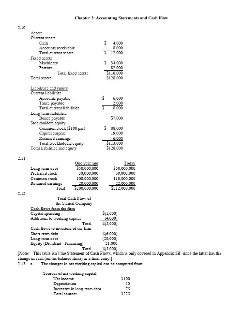
Chapter 2: Accounting Statements and Cash Flow2.10AssetsCurrent assetsCash $ 4,000Accounts receivable 8,000Total current assets $ 12,000Fixed assetsMachinery $ 34,000Patents 82,000Total fixed assets $116,000Total assets $128,000Liabilities and equityCurrent liabilitiesAccounts payable $ 6,000Taxes payable 2,000Total current liabilities $ 8,000Long-term liabilitiesBonds payable $7,000Stockholders equityCommon stock ($100 par) $ 88,000Capital surplus 19,000Retained earnings 6,000Total stockholders equity $113,000Total liabilities and equity $128,0002.11One year ago TodayLong-term debt $50,000,000 $50,000,000Preferred stock 30,000,000 30,000,000Common stock 100,000,000 110,000,000Retained earnings 20,000,000 22,000,000Total $200,000,000 $212,000,0002.12Total Cash Flow ofthe Stancil CompanyCash flows from the firmCapital spending $(1,000)Additions to working capital (4,000)Total $(5,000)Cash flows to investors of the firmShort-term debt $(6,000)Long-term debt (20,000)Equity (Dividend - Financing) 21,000Total $(5,000)[Note: This table isn’t the Statement of Cash Flows, which is only covered in Appendix 2B, since the latter has th e change in cash (on the balance sheet) as a final entry.]2.13 a. The changes in net working capital can be computed from:Sources of net working capitalNet income $100Depreciation 50Increases in long-term debt 75Total sources $225Uses of net working capitalDividends $50Increases in fixed assets* 150Total uses $200Additions to net working capital $25*Includes $50 of depreciation.b.Cash flow from the firmOperating cash flow $150Capital spending (150)Additions to net working capital (25)Total $(25)Cash flow to the investorsDebt $(75)Equity 50Total $(25)Chapter 3: Financial Markets and Net Present Value: First Principles of Finance (Advanced)3.14 $120,000 - ($150,000 - $100,000) (1.1) = $65,0003.15 $40,000 + ($50,000 - $20,000) (1.12) = $73,6003.16 a. ($7 million + $3 million) (1.10) = $11.0 millionb.i. They could spend $10 million by borrowing $5 million today.ii. They will have to spend $5.5 million [= $11 million - ($5 million x 1.1)] at t=1.Chapter 4: Net Present Valuea. $1,000 ⨯ 1.0510 = $1,628.89b. $1,000 ⨯ 1.0710 = $1,967.15c. $1,000 ⨯ 1.0520 = $2,653.30d. Interest compounds on the interest already earned. Therefore, the interest earned inSince this bond has no interim coupon payments, its present value is simply the present value of the $1,000 that will be received in 25 years. Note: As will be discussed in the next chapter, the present value of the payments associated with a bond is the price of that bond.PV = $1,000 /1.125 = $92.30PV = $1,500,000 / 1.0827 = $187,780.23a. At a discount rate of zero, the future value and present value are always the same. Remember, FV =PV (1 + r) t. If r = 0, then the formula reduces to FV = PV. Therefore, the values of the options are $10,000 and $20,000, respectively. You should choose the second option.b. Option one: $10,000 / 1.1 = $9,090.91Option two: $20,000 / 1.15 = $12,418.43Choose the second option.c. Option one: $10,000 / 1.2 = $8,333.33Option two: $20,000 / 1.25 = $8,037.55Choose the first option.d. You are indifferent at the rate that equates the PVs of the two alternatives. You know that rate mustfall between 10% and 20% because the option you would choose differs at these rates. Let r be thediscount rate that makes you indifferent between the options.$10,000 / (1 + r) = $20,000 / (1 + r)5(1 + r)4 = $20,000 / $10,000 = 21 + r = 1.18921r = 0.18921 = 18.921%The $1,000 that you place in the account at the end of the first year will earn interest for six years. The $1,000 that you place in the account at the end of the second year will earn interest for five years, etc. Thus, the account will have a balance of$1,000 (1.12)6 + $1,000 (1.12)5 + $1,000 (1.12)4 + $1,000 (1.12)3= $6,714.61PV = $5,000,000 / 1.1210 = $1,609,866.18a. $1.000 (1.08)3 = $1,259.71b. $1,000 [1 + (0.08 / 2)]2 ⨯ 3 = $1,000 (1.04)6 = $1,265.32c. $1,000 [1 + (0.08 / 12)]12 ⨯ 3 = $1,000 (1.00667)36 = $1,270.24d. $1,000 e0.08 ⨯ 3 = $1,271.25e. The future value increases because of the compounding. The account is earning interest on interest. Essentially, the interest is added to the account balance at the e nd of every compounding period. During the next period, the account earns interest on the new balance. When the compounding period shortens, the balance that earns interest is rising faster.The price of the consol bond is the present value of the coupon payments. Apply the perpetuity formula to find the present value. PV = $120 / 0.15 = $800a. $1,000 / 0.1 = $10,000b. $500 / 0.1 = $5,000 is the value one year from now of the perpetual stream. Thus, the value of theperpetuity is $5,000 / 1.1 = $4,545.45.c. $2,420 / 0.1 = $24,200 is the value two years from now of the perpetual stream. Thus, the value of the perpetuity is $24,200 / 1.12 = $20,000.pply the NPV technique. Since the inflows are an annuity you can use the present value of an annuity factor.ANPV = -$6,200 + $1,200 81.0= -$6,200 + $1,200 (5.3349)= $201.88Yes, you should buy the asset.Use an annuity factor to compute the value two years from today of the twenty payments. Remember, the annuity formula gives you the value of the stream one year before the first payment. Hence, the annuity factor will give you the value at the end of year two of the stream of payments.A= $2,000 (9.8181)Value at the end of year two = $2,000 20.008= $19,636.20The present value is simply that amount discounted back two years.PV = $19,636.20 / 1.082 = $16,834.88The easiest way to do this problem is to use the annuity factor. The annuity factor must be equal to $12,800 / $2,000 = 6.4; remember PV =C A T r. The annuity factors are in the appendix to the text. To use the factor table to solve this problem, scan across the row labeled 10 years until you find 6.4. It is close to the factor for 9%, 6.4177. Thus, the rate you will receive on this note is slightly more than 9%.You can find a more precise answer by interpolating between nine and ten percent.[ 10% ⎤[6.1446 ⎤a ⎡r ⎥bc ⎡6.4 ⎪ d⎣9%⎦⎣6.4177 ⎦By interpolating, you are presuming that the ratio of a to b is equal to the ratio of c to d.(9 - r ) / (9 - 10) = (6.4177 - 6.4 ) / (6.4177 - 6.1446)r = 9.0648%The exact value could be obtained by solving the annuity formula for the interest rate. Sophisticated calculators can compute the rate directly as 9.0626%.[Note: A standard financial calculator’s TVM keys can solve for this rate. With annuity flows, the IRR key on “advanced” financial c alculators is unnecessary.]a. The annuity amount can be computed by first calculating the PV of the $25,000 which youThat amount is $17,824.65 [= $25,000 / 1.075]. Next compute the annuity which has the same present value.A$17,824.65 = C 507.0$17,824.65 = C (4.1002)C = $4,347.26Thus, putting $4,347.26 into the 7% account each year will provide $25,000 five years from today.b. The lump sum payment must be the present value of the $25,000, i.e., $25,000 / 1.075 =$17,824.65The formula for future value of any annuity can be used to solve the problem (see footnote 11 of the text).Option one: This cash flow is an annuity due. To value it, you must use the after-tax amounts. Theafter-tax payment is $160,000 (1 - 0.28) = $115,200. Value all except the first payment using the standard annuity formula, then add back the first payment of $115,200 to obtain the value of this option.AValue = $115,200 + $115,200 30.010= $115,200 + $115,200 (9.4269)= $1,201,178.88Option two: This option is valued similarly. You are able to have $446,000 now; this is already on an after-tax basis. You will receive an annuity of $101,055 for each of the next thirty years. Those payments are taxable when you receive them, so your after-tax payment is $72,759.60 [= $101,055 (1 - 0.28)].AValue = $446,000 + $72,759.60 30.010= $446,000 + $72,759.60 (9.4269)= $1,131,897.47Since option one has a higher PV, you should choose it.et r be the rate of interest you must earn.$10,000(1 + r)12 = $80,000(1 + r)12= 8r = 0.18921 = 18.921%First compute the present value of all the payments you must make for your children’s educati on. The value as of one year before matriculation of one child’s education isA= $21,000 (2.8550) = $59,955.$21,000 415.0This is the value of the elder child’s education fourteen years from now. It is the value of the younger child’s education sixteen years from today. The present value of these isPV = $59,955 / 1.1514 + $59,955 / 1.1516= $14,880.44You want to make fifteen equal payments into an account that yields 15% so that the present value of the equal payments is $14,880.44.A= $14,880.44 / 5.8474 = $2,544.80Payment = $14,880.44 / 15.015This problem applies the growing annuity formula. The first payment is$50,000(1.04)2(0.02) = $1,081.60.PV = $1,081.60 [1 / (0.08 - 0.04) - {1 / (0.08 - 0.04)}{1.04 / 1.08}40]= $21,064.28This is the present value of the payments, so the value forty years from today is$21,064.28 (1.0840) = $457,611.46se the discount factors to discount the individual cash flows. Then compute the NPV of the project. NoticeYou can still use the factor tables to compute their PV. Essentially, they form cash flows that are a six year annuity less a two year annuity. Thus, the appropriate annuity factor to use with them is 2.6198 (= 4.3553 - 1.7355).Year Cash Flow Factor PV0.9091 $636.371$70020.8264 743.769003 1,000 ⎤4 1,000 ⎥ 2.6198 2,619.805 1,000 ⎥6 1,000 ⎦7 1,250 0.5132 641.508 1,375 0.4665 641.44Total $5,282.87NPV = -$5,000 + $5,282.87= $282.87Purchase the machine.Chapter 5: How to Value Bonds and StocksThe amount of the semi-annual interest payment is $40 (=$1,000 ⨯ 0.08 / 2). There are a total of 40 periods;i.e., two half years in each of the twenty years in the term to maturity. The annuity factor tables can be usedto price these bonds. The appropriate discount rate to use is the semi-annual rate. That rate is simply the annual rate divided by two. Thus, for part b the rate to be used is 5% and for part c is it 3%.A+F/(1+r)40PV=C Tra. $40 (19.7928) + $1,000 / 1.0440 = $1,000Notice that whenever the coupon rate and the market rate are the same, the bond is priced at par.b. $40 (17.1591) + $1,000 / 1.0540 = $828.41Notice that whenever the coupon rate is below the market rate, the bond is priced below par.c. $40 (23.1148) + $1,000 / 1.0340 = $1,231.15Notice that whenever the coupon rate is above the market rate, the bond is priced above par.a. The semi-annual interest rate is $60 / $1,000 = 0.06. Thus, the effective annual rate is 1.062 - 1 =0.1236 = 12.36%.A+ $1,000 / 1.0612b. Price = $30 12.006= $748.48A+ $1,000 / 1.0412c. Price = $30 1204.0= $906.15Note: In parts b and c we are implicitly assuming that the yield curve is flat. That is, the yield in year 5applies for year 6 as well.rice = $2 (0.72) / 1.15 + $4 (0.72) / 1.152 + $50 / 1.153= $36.31The number of shares you own = $100,000 / $36.31 = 2,754 sharesPrice = $1.15 (1.18) / 1.12 + $1.15 (1.182) / 1.122 + $1.152 (1.182) / 1.123+ {$1.152 (1.182)(1.06) / (0.12 - 0.06)} / 1.123= $26.95[Insert before last sentence of question: Assume that dividends are a fixed proportion of earnings.] Dividend one year from now = $5 (1 - 0.10) = $4.50Price = $5 + $4.50 / {0.14 - (-0.10)}= $23.75Since the current $5 dividend has not yet been paid, it is still included in the stock price.Chapter 6: Some Alternative Investment Rulesa. Payback period of Project A = 1 + ($7,500 - $4,000) / $3,500 = 2 yearsPayback period of Project B = 2 + ($5,000 - $2,500 -$1,200) / $3,000 = 2.43 yearsProject A should be chosen.b. NPV A = -$7,500 + $4,000 / 1.15 + $3,500 / 1.152 + $1,500 / 1.153 = -$388.96NPV B = -$5,000 + $2,500 / 1.15 + $1,200 / 1.152 + $3,000 / 1.153 = $53.83Project B should be chosen.a. Average Investment:($16,000 + $12,000 + $8,000 + $4,000 + 0) / 5 = $8,000Average accounting return:$4,500 / $8,000 = 0.5625 = 56.25%b. 1. AAR does not consider the timing of the cash flows, hence it does not consider the timevalue of money.2. AAR uses an arbitrary firm standard as the decision rule.3. AAR uses accounting data rather than net cash flows.aAverage Investment = (8000 + 4000 + 1500 + 0)/4 = 3375.00Average Net Income = 2000(1-0.75) = 1500=> AAR = 1500/3375=44.44%a. Solve x by trial and error:-$8,000 + $4,000 / (1 + x) + $3000 / (1 + x)2 + $2,000 / (1 + x)3 = 0x = 6.93%b. No, since the IRR (6.93%) is less than the discount rate of 8%.Alternatively, the NPV @ a discount rate of 0.08 = -$136.62.a. Solve r in the equation:$5,000 - $2,500 / (1 + r) - $2,000 / (1 + r)2 - $1,000 / (1 + r)3- $1,000 / (1 + r)4 = 0By trial and error,IRR = r = 13.99%b. Since this problem is the case of financing, accept the project if the IRR is less than the required rate of return.IRR = 13.99% > 10%Reject the offer.c. IRR = 13.99% < 20%Accept the offer.d. When r = 10%:NPV = $5,000 - $2,500 / 1.1 - $2,000 / 1.12 - $1,000 / 1.13 - $1,000 / 1.14When r = 20%:NPV = $5,000 - $2,500 / 1.2 - $2,000 / 1.22 - $1,000 / 1.23 - $1,000 / 1.24= $466.82Yes, they are consistent with the choices of the IRR rule since the signs of the cash flows change only once.A/ $160,000 = 1.04PI = $40,000 715.0Since the PI exceeds one accept the project.Chapter 7: Net Present Value and Capital BudgetingSince there is uncertainty surrounding the bonus payments, which McRae might receive, you must use the expected value of McRae’s bonuses in the computation of the PV of his contract. McRae’s salary plus the expected value of his bonuses in years one through three is$250,000 + 0.6 ⨯ $75,000 + 0.4 ⨯ $0 = $295,000.Thus the total PV of his three-year contract isPV = $400,000 + $295,000 [(1 - 1 / 1.12363) / 0.1236]+ {$125,000 / 1.12363} [(1 - 1 / 1.123610 / 0.1236]= $1,594,825.68EPS = $800,000 / 200,000 = $4NPVGO = (-$400,000 + $1,000,000) / 200,000 = $3Price = EPS / r + NPVGO= $4 / 0.12 + $3=$36.33Year 0 Year 1 Year 2 Year 3 Year 4 Year 51. Annual Salary$120,000 $120,000 $120,000 $120,000 $120,000 Savings2. Depreciation 100,000 160,000 96,000 57,600 57,6003. Taxable Income 20,000 -40,000 24,000 62,400 62,4004. Taxes 6,800 -13,600 8,160 21,216 21,2165. Operating Cash Flow113,200 133,600 111,840 98,784 98,784 (line 1-4)$100,000 -100,0006. ∆ Net workingcapital7. Investment $500,000 75,792*8. Total Cash Flow -$400,000 $113,200 $133,600 $111,840 $98,784 $74,576*75,792 = $100,000 - 0.34 ($100,000 - $28,800)NPV = -$400,000+ $113,200 / 1.12 + $133,600 / 1.122 + $111,840 / 1.123+ $98,784 / 1.124 + $74,576 / 1.125= -$7,722.52Real interest rate = (1.15 / 1.04) - 1 = 10.58%NPV A = -$40,000+ $20,000 / 1.1058 + $15,000 / 1.10582 + $15,000 / 1.10583= $1,446.76NPV B = -$50,000+ $10,000 / 1.15 + $20,000 / 1.152 + $40,000 / 1.153= $119.17Choose project A.PV = $120,000 / {0.11 - (-0.06)}t = 0 t = 1 t = 2 t = 3 t = 4 t = 5 t = 6 ...$12,000 $6,000 $6,000 $6,000$4,000$12,000 $6,000 $6,000 ...The present value of one cycle is:A+ $4,000 / 1.064PV = $12,000 + $6,000 306.0= $12,000 + $6,000 (2.6730) + $4,000 / 1.064= $31,206.37The cycle is four years long, so use a four year annuity factor to compute the equivalent annual cost (EAC).AEAC = $31,206.37 / 406.0= $31,206.37 / 3.4651= $9,006The present value of such a stream in perpetuity is$9,006 / 0.06 = $150,100o evaluate the word processors, compute their equivalent annual costs (EAC).BangAPV(costs) = (10 ⨯ $8,000) + (10 ⨯ $2,000) 414.0= $80,000 + $20,000 (2.9137)= $138,274EAC = $138,274 / 2.9137= $47,456IOUAPV(costs) = (11 ⨯ $5,000) + (11 ⨯ $2,500) 3.014- (11 ⨯ $500) / 1.143= $55,000 + $27,500 (2.3216) - $5,500 / 1.143= $115,132EAC = $115,132 / 2.3216= $49,592BYO should purchase the Bang word processors.Chapter 8: Strategy and Analysis in Using Net Present ValueThe accounting break-even= (120,000 + 20,000) / (1,500 - 1,100)= 350 units. The accounting break-even= 340,000 / (2.00 - 0.72)= 265,625 abalonesb. [($2.00 ⨯ 300,000) - (340,000 + 0.72 ⨯ 300,000)] (0.65)= $28,600This is the after tax profit.Chapter 9: Capital Market Theory: An Overviewa. Capital gains = $38 - $37 = $1 per shareb. Total dollar returns = Dividends + Capital Gains = $1,000 + ($1*500) = $1,500 On a per share basis, this calculation is $2 + $1 = $3 per sharec. On a per share basis, $3/$37 = 0.0811 = 8.11% On a total dollar basis, $1,500/(500*$37) = 0.0811 = 8.11%d. No, you do not need to sell the shares to include the capital gains in the computation of the returns. The capital gain is included whether or not you realize the gain. Since you could realize the gain if you choose, you should include it.The expected holding period return is:()[]%865.1515865.052$/52$75.54$50.5$==-+There appears to be a lack of clarity about the meaning of holding period returns. The method used in the answer to this question is the one used in Section 9.1. However, the correspondence is not exact, because in this question, unlike Section 9.1, there are cash flows within the holding period. The answer above ignores the dividend paid in the first year. Although the answer above technically conforms to the eqn at the bottom of Fig. 9.2, the presence of intermediate cash flows that aren’t accounted for renders th is measure questionable, at best. There is no similar example in the body of the text, and I have never seen holding period returns calculated in this way before.Although not discussed in this book, there are two generally accepted methods of computing holding period returns in the presence of intermediate cash flows. First, the time weighted return calculates averages (geometric or arithmetic) of returns between cash flows. Unfortunately, that method can’t be used here, because we are not given the va lue of the stock at the end of year one. Second, the dollar weighted measure calculates the internal rate of return over the entire holding period. Theoretically, that method can be applied here, as follows: 0 = -52 + 5.50/(1+r) + 60.25/(1+r)2 => r = 0.1306.This produces a two year holding period return of (1.1306)2 – 1 = 0.2782. Unfortunately, this book does not teach the dollar weighted method.In order to salvage this question in a financially meaningful way, you would need the value of the stock at the end of one year. Then an illustration of the correct use of the time-weighted return would be appropriate. A complicating factor is that, while Section 9.2 illustrates the holding period return using the geometric return for historical data, the arithmetic return is more appropriate for expected future returns.E(R) = T-Bill rate + Average Excess Return = 6.2% + (13.0% -3.8%) = 15.4%. Common Treasury Realized Stocks Bills Risk Premium -7 32.4% 11.2% 21.2%-6 -4.9 14.7 -19.6-5 21.4 10.5 10.9 -4 22.5 8.8 13.7 -3 6.3 9.9 -3.6 -2 32.2 7.7 24.5 Last 18.5 6.2 12.3 b. The average risk premium is 8.49%.49.873.125.246.37.139.106.192.21=++-++- c. Yes, it is possible for the observed risk premium to be negative. This can happen in any single year. The.b.Standard deviation = 03311.0001096.0=.b.Standard deviation = = 0.03137 = 3.137%.b.Chapter 10: Return and Risk: The Capital-Asset-Pricing Model (CAPM)a. = 0.1 (– 4.5%) + 0.2 (4.4%) + 0.5 (12.0%) + 0.2 (20.7%) = 10.57%b.σ2 = 0.1 (–0.045 – 0.1057)2 + 0.2 (0.044 – 0.1057)2 + 0.5 (0.12 – 0.1057)2+ 0.2 (0.207 – 0.1057)2 = 0.0052σ = (0.0052)1/2 = 0.072 = 7.20%Holdings of Atlas stock = 120 ⨯ $50 = $6,000 ⨯ $20 = $3,000Weight of Atlas stock = $6,000 / $9,000 = 2 / 3Weight of Babcock stock = $3,000 / $9,000 = 1 / 3a. = 0.3 (0.12) + 0.7 (0.18) = 0.162 = 16.2%σP 2= 0.32 (0.09)2 + 0.72 (0.25)2 + 2 (0.3) (0.7) (0.09) (0.25) (0.2)= 0.033244σP= (0.033244)1/2 = 0.1823 = 18.23%a.State Return on A Return on B Probability1 15% 35% 0.4 ⨯ 0.5 = 0.22 15% -5% 0.4 ⨯ 0.5 = 0.23 10% 35% 0.6 ⨯ 0.5 = 0.34 10% -5% 0.6 ⨯ 0.5 = 0.3b. = 0.2 [0.5 (0.15) + 0.5 (0.35)] + 0.2[0.5 (0.15) + 0.5 (-0.05)]+ 0.3 [0.5 (0.10) + 0.5 (0.35)] + 0.3 [0.5 (0.10) + 0.5 (-0.05)]= 0.135= 13.5%Note: The solution to this problem requires calculus.Specifically, the solution is found by minimizing a function subject to a constraint. Calculus ability is not necessary to understand the principles behind a minimum variance portfolio.Min { X A2 σA2 + X B2σB2+ 2 X A X B Cov(R A , R B)}subject to X A + X B = 1Let X A = 1 - X B. Then,Min {(1 - X B)2σA2 + X B2σB2+ 2(1 - X B) X B Cov (R A, R B)}Take a derivative with respect to X B.d{∙} / dX B = (2 X B - 2) σA2+ 2 X B σB2 + 2 Cov(R A, R B) - 4 X B Cov(R A, R B)Set the derivative equal to zero, cancel the common 2 and solve for X B.X BσA2- σA2+ X B σB2 + Cov(R A, R B) - 2 X B Cov(R A, R B) = 0X B = {σA2 - Cov(R A, R B)} / {σA2+ σB2 - 2 Cov(R A, R B)}andX A = {σB2 - Cov(R A, R B)} / {σA2+ σB2 - 2 Cov(R A, R B)}Using the data from the problem yields,X A = 0.8125 andX B = 0.1875.a. Using the weights calculated above, the expected return on the minimum variance portfolio isE(R P) = 0.8125 E(R A) + 0.1875 E(R B)= 0.8125 (5%) + 0.1875 (10%)= 5.9375%b. Using the formula derived above, the weights areX A = 2 / 3 andX B = 1 / 3c. The variance of this portfolio is zero.σP 2= X A2 σA2 + X B2σB2+ 2 X A X B Cov(R A , R B)= (4 / 9) (0.01) + (1 / 9) (0.04) + 2 (2 / 3) (1 / 3) (-0.02)= 0This demonstrates that assets can be combined to form a risk-free portfolio.14.2%= 3.7%+β(7.5%) ⇒β = 1.40.25 = R f + 1.4 [R M– R f] (I)0.14 = R f + 0.7 [R M– R f] (II)(I) – (II)=0.11 = 0.7 [R M– R f] (III)[R M– R f ]= 0.1571Put (III) into (I) 0.25 = R f + 1.4[0.1571]R f = 3%[R M– R f ]= 0.1571R M = 0.1571 + 0.03= 18.71%a. = 4.9% + βi (9.4%)βD= Cov(R D, R M) / σM 2 = 0.0635 / 0.04326 = 1.468= 4.9 + 1.468 (9.4) = 18.70%Weights:X A = 5 / 30 = 0.1667X B = 10 / 30 = 0.3333X C = 8 / 30 = 0.2667X D = 1 - X A - X B - X C = 0.2333Beta of portfolio= 0.1667 (0.75) + 0.3333 (1.10) + 0.2667 (1.36) + 0.2333 (1.88)= 1.293= 4 + 1.293 (15 - 4) = 18.22%a. (i) βA= ρA,MσA / σMρA,M= βA σM / σA= (0.9) (0.10) / 0.12= 0.75(ii) σB= βB σM / ρB,M= (1.10) (0.10) / 0.40= 0.275(iii) βC= ρC,MσC / σM= (0.75) (0.24) / 0.10= 1.80(iv) ρM,M= 1(v) βM= 1(vi) σf= 0(vii) ρf,M= 0(viii) βf= 0b. SML:E(R i) = R f + βi {E(R M) - R f}= 0.05 + (0.10) βiSecurity βi E(R i)A 0.13 0.90 0.14B 0.16 1.10 0.16C 0.25 1.80 0.23Security A performed worse than the market, while security C performed better than the market.Security B is fairly priced.c. According to the SML, security A is overpriced while security C is under-priced. Thus, you could invest in security C while sell security A (if you currently hold it).a. The typical risk-averse investor seeks high returns and low risks. To assess thetwo stocks, find theReturns:State of economy ProbabilityReturn on A*Recession 0.1 -0.20 Normal 0.8 0.10 Expansion0.10.20* Since security A pays no dividend, the return on A is simply (P 1 / P 0) - 1. = 0.1 (-0.20) + 0.8 (0.10) + 0.1 (0.20) = 0.08 = 0.09 This was given in the problem.Risk:R A - (R A -)2 P ⨯ (R A -)2 -0.28 0.0784 0.00784 0.02 0.0004 0.00032 0.12 0.0144 0.00144 Variance 0.00960Standard deviation (R A ) = 0.0980βA = {Corr(R A , R M ) σ(R A )} / σ(R M ) = 0.8 (0.0980) / 0.10= 0.784βB = {Corr(R B , R M ) σ(R B )} / σ(R M ) = 0.2 (0.12) / 0.10= 0.24The return on stock B is higher than the return on stock A. The risk of stock B, as measured by itsbeta, is lower than the risk of A. Thus, a typical risk-averse investor will prefer stock B.b. = (0.7) + (0.3) = (0.7) (0.8) + (0.3) (0.09) = 0.083σP 2= 0.72 σA 2 + 0.32 σB 2 + 2 (0.7) (0.3) Corr (R A , R B ) σA σB = (0.49) (0.0096) + (0.09) (0.0144) + (0.42) (0.6) (0.0980) (0.12) = 0.0089635 σP = = 0.0947 c. The beta of a portfolio is the weighted average of the betas of the components of the portfolio. βP = (0.7) βA + (0.3) βB = (0.7) (0.784) + (0.3) (0.240) = 0.621Chapter 11:An Alternative View of Risk and Return: The Arbitrage Pricing Theorya. Stock A:()()R R R R R A A A m m Am A=+-+=+-+βεε105%12142%...Stock B:()()R R R R R B B m m Bm B=+-+=+-+βεε130%098142%...Stock C:()R R R R R C C C m m Cm C=+-+=+-+βεε157%137142%)..(.b.()[]()[]()[]()()()()()()[]()()CB A m cB A m c m B m A m CB A P 25.045.030.0%2.14R 1435.1%925.1225.045.030.0%2.14R 37.125.098.045.02.130.0%7.1525.0%1345.0%5.1030.0%2.14R 37.1%7.1525.0%2.14R 98.0%0.1345.0%2.14R 2.1%5.1030.0R 25.0R 45.0R 30.0R ε+ε+ε+-+=ε+ε+ε+-+++++=ε+-++ε+-++ε+-+=++= c.i.()R R R A B C =+-==+-==+-=105%1215%142%)1113%09815%142%)137%157%13715%142%168%..(..46%.(......ii.R P =+-=12925%1143515%142%)138398%..(..To determine which investment investor would prefer, you must compute the variance of portfolios created bymany stocks from either market. Note, because you know that diversification is good, it is reasonable to assume that once an investor chose the market in which he or she will invest, he or she will buy many stocks in that market.Known:E EF ====001002 and and for all i.i σσεε..Assume: The weight of each stock is 1/N; that is, X N i =1/for all i.If a portfolio is composed of N stocks each forming 1/N proportion of the portfolio, the return on the portfolio is 1/N times the sum of the returns on the N stocks. Recall that the return on each stock is 0.1+βF+ε.()()()()()()[]()()()()()()()[]()[]()[]()()[]()()()()()j i 2j i 22j i i 2222222222P P P P iP ,0.04Corr 0.01,Cov s =isvariance the ,N as limit In the ,Cov 1/N 1s 1/N s )(1/N 1/N F 2F E 1/N F E 0.10.1/N F 0.1E R E R E R Var 0.101/N 00.1E 1/N F E 0.11/N F 0.1E R E 1/N F 0.1F 0.1(1/N)R 1/N R εε+β=εε+β∞⇒εε-+ε+β=ε∑+εβ+β=ε+β=-ε+β+=-==+β+=ε+β+=ε∑+β+=ε+β+=ε+β+==∑∑∑∑∑∑∑∑()()()()()()Thus,F R f E R E R Var R Corr Var R Corr ii ip P p i j PijR 1i =++=++===+=+010*********002250040002500412212111222.........,,εεεεεεa.()()()()Corr Corr Var R Var R i j i j p pεεεε112212000225000225,,..====Since Var ()()R p 1 Var R 2p 〉, a risk averse investor will prefer to invest in the second market.b. Corr ()()εεεε112090i j j ,.,== and Corr 2i()()Var R Var R pp120058500025==..。
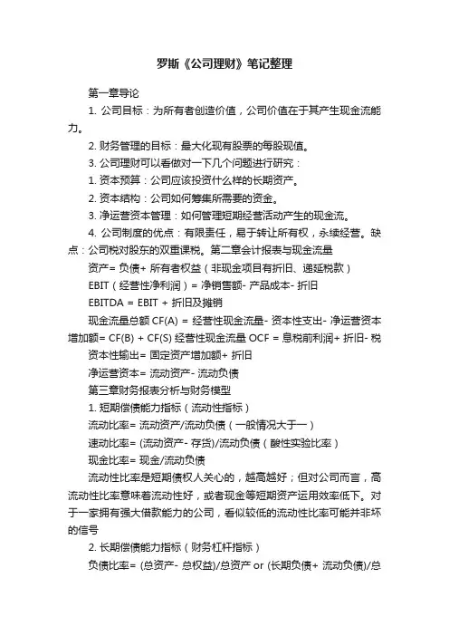
罗斯《公司理财》笔记整理第一章导论1. 公司目标:为所有者创造价值,公司价值在于其产生现金流能力。
2. 财务管理的目标:最大化现有股票的每股现值。
3. 公司理财可以看做对一下几个问题进行研究:1. 资本预算:公司应该投资什么样的长期资产。
2. 资本结构:公司如何筹集所需要的资金。
3. 净运营资本管理:如何管理短期经营活动产生的现金流。
4. 公司制度的优点:有限责任,易于转让所有权,永续经营。
缺点:公司税对股东的双重课税。
第二章会计报表与现金流量资产= 负债+ 所有者权益(非现金项目有折旧、递延税款)EBIT(经营性净利润)= 净销售额- 产品成本- 折旧EBITDA = EBIT + 折旧及摊销现金流量总额CF(A) = 经营性现金流量- 资本性支出- 净运营资本增加额= CF(B) + CF(S) 经营性现金流量OCF = 息税前利润+ 折旧- 税资本性输出= 固定资产增加额+ 折旧净运营资本= 流动资产- 流动负债第三章财务报表分析与财务模型1. 短期偿债能力指标(流动性指标)流动比率= 流动资产/流动负债(一般情况大于一)速动比率= (流动资产- 存货)/流动负债(酸性实验比率)现金比率= 现金/流动负债流动性比率是短期债权人关心的,越高越好;但对公司而言,高流动性比率意味着流动性好,或者现金等短期资产运用效率低下。
对于一家拥有强大借款能力的公司,看似较低的流动性比率可能并非坏的信号2. 长期偿债能力指标(财务杠杆指标)负债比率= (总资产- 总权益)/总资产or (长期负债+ 流动负债)/总资产权益乘数= 总资产/总权益= 1 + 负债权益比利息倍数= EBIT/利息现金对利息的保障倍数(Cash coverage radio) = EBITDA/利息3. 资产管理或资金周转指标存货周转率= 产品销售成本/存货存货周转天数= 365天/存货周转率应收账款周转率= (赊)销售额/应收账款总资产周转率= 销售额/总资产= 1/资本密集度4. 盈利性指标销售利润率= 净利润/销售额资产收益率ROA = 净利润/总资产权益收益率ROE = 净利润/总权益5. 市场价值度量指标市盈率= 每股价格/每股收益EPS 其中EPS = 净利润/发行股票数市值面值比= 每股市场价值/每股账面价值企业价值EV = 公司市值+ 有息负债市值- 现金EV乘数= EV/EBITDA6. 杜邦恒等式ROE = 销售利润率(经营效率)x总资产周转率(资产运用效率)x权益乘数(财杠)ROA = 销售利润率x总资产周转率7. 销售百分比法假设项目随销售额变动而成比例变动,目的在于提出一个生成预测财务报表的快速实用方法。


第十一章:收益和风险:资本资产定价模型1.系统性风险通常是不可分散的,而非系统性风险是可分散的。
但是,系统风险是可以控制的,这需要很大的降低投资者的期望收益。
2.(1)系统性风险(2)非系统性风险(3)都有,但大多数是系统性风险(4)非系统性风险(5)非系统性风险(6)系统性风险3.否,应在两者之间4.错误,单个资产的方差是对总风险的衡量。
5.是的,组合标准差会比组合中各种资产的标准差小,但是投资组合的贝塔系数不会小于最小的贝塔值。
6. 可能为0,因为当贝塔值为0 时,贝塔值为0 的风险资产收益=无风险资产的收益,也可能存在负的贝塔值,此时风险资产收益小于无风险资产收益。
7.因为协方差可以衡量一种证券与组合中其他证券方差之间的关系。
8. 如果我们假设,在过去3 年市场并没有停留不变,那么南方公司的股价价格缺乏变化表明该股票要么有一个标准差或贝塔值非常接近零。
德州仪器的股票价格变动大并不意味着该公司的贝塔值高,只能说德州仪器总风险很高。
9. 石油股票价格的大幅度波动并不表明这些股票是一个很差的投资。
如果购买的石油股票是作为一个充分多元化的产品组合的一部分,它仅仅对整个投资组合做出了贡献。
这种贡献是系统风险或β来衡量的。
所以,是不恰当的。
10. The statement is false. If a security has a negative beta, investors would want to hold the asset to reduce the variability of their portfolios. Those assets will have expected returns that are lower than the risk-free rate. To see this, examine the Capital Asset Pricing Model:E(R S) = R f + S[E(R M) – R f] If S < 0, then the E(R S) < R f11. Total value = 95($53) + 120($29) = $8,515The portfolio weight for each stock is:WeightA = 95($53)/$8,515 = .5913 WeightB = 120($29)/$8,515 = .4087 12.Total value = $1,900 + 2,300 = $4,200So, the expected return of this portfolio is:E(R p) = ($1,900/$4,200)(0.10) + ($2,300/$4,200)(0.15) = .1274 or 12.74%13. E(R p) = .40(.11) + .35(.17) + .25(.14) = .1385 or 13.85%14. Here we are given the expected return of the portfolio and the expected return of each asset in the portfolio and are asked to find the weight of each asset. We can use the equation for the expected return of a portfolio to solve this problem. Since the total weight of a portfolio must equal 1 (100%), the weight of Stock Y must be one minus the weight of Stock X. Mathematically speaking, this means:E(R p) = .129 = .16w X + .10(1 –w X)We can now solve this equation for the weight of Stock X as:.129 = .16w X + .10 – .10w X w X = 0.4833So, the dollar amount invested in Stock X is the weight of Stock X times the total portfolio value, or: Investment in X = 0.4833($10,000) = $4,833.33And the dollar amount invested in Stock Y is:Investment in Y = (1 – 0.4833)($10,000) = $5,166.6715. E(R) = .2(–.09) + .5(.11) + .3(.23) = .1060 or 10.60%16. E(RA) = .15(.06) + .65(.07) + .20(.11) = .0765 or 7.65%E(RB) = .15(–.2) + .65(.13) + .20(.33) = .1205 or 12.05%17. E(R A) = .10(–.045) + .25 (.044) + .45(.12) + .20(.207) = .1019 or 10.19%方差=.10(–.045 – .1019)⌒2 + .25(.044 – .1019)⌒2 + .45(.12 – .1019)⌒2 + .20(.207 – .1019)⌒2 = .00535标准差= (.00535)1/2 = .0732 or 7.32%18. E(R p) = .15(.08) + .65(.15) + .20(.24) = .1575 or 15.75%If we own this portfolio, we would expect to get a return of 15.75 percent.19. a.Boom: E(R p) = (.07 + .15 + .33)/3 = .1833 or 18.33%Bust: E(R p) = (.13 + .03 .06)/3 = .0333 or 3.33%E(Rp) = .80(.1833) + .20(.0333) = .1533 or 15.33%b. Boom: E(R p)=.20(.07) +.20(.15) + .60(.33) =.2420 or 24.20%Bust: E(R p) =.20(.13) +.20(.03) + .60( .06) = –.0040 or –0.40%E(R p) = .80(.2420) + .20( .004) = .1928 or 19.28%P的方差= .80(.2420 – .1928)⌒2 + .20( .0040 – .1928)⌒2 = .0096820.a.Boom: E(R p) = .30(.3) + .40(.45) + .30(.33) = .3690 or 36.90%Good: E(R p) = .30(.12) + .40(.10) + .30(.15) = .1210 or 12.10%Poor: E(R p) = .30(.01) + .40(–.15) + .30(–.05) = –.0720 or –7.20%Bust: E(R p) = .30(–.06) + .40(–.30) + .30(–.09) = –.1650 or –16.50%E(R p) = .20(.3690) + .35(.1210) + .30(–.0720) + .15(–.1650) = .0698 or 6.98%b. p⌒2 = .20(.3690 – .0698)⌒2 + .35(.1210 – .0698)⌒2 + .30(–.0720 – .0698)⌒2 + .15(–.1650 – .0698)⌒2 = .03312p的标准差= (.03312)⌒1/2 = .1820 or 18.20%21. β= .25(.75) + .20(1.90) + .15(1.38) + .40(1.16) = 1.2422.βp = 1.0 = 1/3(0) + 1/3(1.85) + 1/3(βX) βX = 1.1523.E(R i) = R f + [E(R M) – R f] ×βiE(R i) = .05 + (.12 – .05)(1.25) = .1375 or 13.75%24. We are given the values for the CAPM except for the of the stock. We need to substitute these values into the CAPM, and solve for the of the stock. One important thing we need to realize is that we are given the market risk premium. The market risk premium is the expected return of the market minus the risk-free rate. We must be careful not to use this value as the expected return of the market. Using the CAPM, we find:E(R i) = .142 = .04 + .07βi 则βi = 1.4625. E(R i) = .105 = .055 + [E(R M) – .055](.73) 则E(R M) = .1235 or 12.35%26. E(R i) = .162 = R f + (.11 – R f)(1.75).162 = R f + .1925 – 1.75R f则R f = .0407 or 4.07%27. a. E(R p) = (.103 + .05)/2 = .0765 or 7.65%b. We need to find the portfolio weights that result in a portfolio with a of 0.50. We know the 贝塔of the risk-free asset is zero. We also know the weight of the risk-free asset is one minus the weight of the stock since the portfolio weights must sum to one, or 100 percent. So:c. We need to find the portfolio weights that result in a portfolio with an expected return of 9 percent. We also know the weight of the risk-free asset is one minus the weight of the stock since the portfolio weights must sum to one, or 100 percent. So:d. Solving for the of the portfolio as we did in part a, we find:18. ßp = w W(1.3) + (1 –w W)(0) = 1.3w WSo, to find the βof the portfolio for any weight of the stock, we simply multiply the weight of the stock times its β.Even though we are solving for the and expected return of a portfolio of one stock and the risk-free asset for different portfolio weights, we are really solving for the SML. Any combination of this stock and the risk-free asset will fall on the SML. For that matter, a portfolio of any stock and the risk-free asset, or any portfolio of stocks, will fall on the SML. We know the slope of the SML line is the market risk premium, so using the CAPM and the information concerning this stock, the market risk premium is:E(R W) = .138 = .05 + MRP(1.30)MRP = .088/1.3 = .0677 or 6.77%So, now we know the CAPM equation for any stock is:E(R p) = .05 + .0677*贝塔p29. E(R Y) = .055 + .068(1.35) = .1468 or 14.68%E(R Z) = .055 + .068(0.85) = .1128 or 11.28%Reward-to-risk ratio Y = (.14 – .055) / 1.35 = .0630Reward-to-risk ratio Z = (.115 – .055) / .85 = .070630. (.14 – R f)/1.35 = (.115 – R f)/0.85We can cross multiply to get: 0.85(.14 – R f) = 1.35(.115 – R f)Solving for the risk-free rate, we find:0.119 – 0.85R f = 0.15525 – 1.35R f R f = .0725 or 7.25%31.32. [E(R A) – R f]/ A = [E(R B) – R f]/ßBRP A/β A = RP B/β B βB/βA = RP B/RP A33. Boom: E(R p) = .4(.20) + .4(.35) + .2(.60) = .3400 or 34.00%Normal: E(R p) = .4(.15) + .4(.12) + .2(.05) = .1180 or 11.80%Bust: E(R p) = .4(.01) + .4(–.25) + .2(–.50) = –.1960 or –19.60%E(R p) = .35(.34) + .40(.118) + .25(–.196) = .1172 or 11.72%σp⌒2= .35(.34 – .1172)2 + .40(.118 – .1172)2 + .25(–.196 – .1172)2 = .04190σp= (.04190)1/2 = .2047 or 20.47%b. RP i = E(R p) – R f = .1172 – .038 = .0792 or 7.92%c.Approximate expected real return = .1172 – .035 = .0822 or 8.22%1 + E(R i) = (1 + h)[1 + e(r i)]1.1172 = (1.0350)[1 + e(r i)]e(r i) = (1.1172/1.035) – 1 = .0794 or 7.94%Approximate expected real risk premium = .0792 – .035 = .0442 or 4.42%Exact expected real risk premium = (1.0792/1.035) – 1 = .0427 or 4.27%34. w A = $180,000 / $1,000,000 = .18 w B = $290,000/$1,000,000 = .29βp = 1.0 = w A(.75) + w B(1.30) + w C(1.45) + w Rf(0) w C = .33655172Invest in Stock C = .33655172($1,000,000) = $336,551.721 = w A + w B + w C + w Rf 1 = .18 + .29 + .33655172 + w Rf w Rf = .19344828Invest in risk-free asset = .19344828($1,000,000) = $193,448.28w X(.172) + w Y(.0875) + (1 –w X –w Y)(.055)35. E(R p) = .1070 =βp = .8 = w X(1.8) + w Y(0.50) + (1 –w X – w Y)(0)w X = –0.11111 w Y = 2.00000 w Rf = –0.88889Investment in stock X = –0.11111($100,000) = –$11,111.1136. E(R A) = .33(.082) + .33(.095) + .33(.063) = .0800 or 8.00%E(R B) = .33(–.065) + .33(.124) + .33(.185) = .0813 or 8.13%股票A:方差=.33(.082 – .0800)⌒2 + .33(.095 – .0800)⌒2 + .33(.063 – .0800)⌒2 = .00017 标准差=(.00017)⌒1/2 = .0131 or 1.31%股票B:方差=.33(–.065 – .0813)⌒2 + .33(.124 – .0813)⌒2 + .33(.185 – .0813)⌒2 = .01133 标准差= (.01133)1/2 = .1064 or 1064%Cov(A,B) = .33(.092 – .0800)(–.065 – .0813) + .33(.095 – .0800)(.124 – .0813) + .33(.063– .0800)(.185 – .0813) = –.000472ρA,B = Cov(A,B) / (标准差A 标准差B)= –.000472 / (.0131)(.1064) = –.337337. E(R A) = .30(–.020) + .50(.138) + .20(.218) = .1066 or 10.66%E(R B) = .30(.034) + .50(.062) + .20(.092) = .0596 or 5.96%A的方差 =.30(–.020 – .1066)⌒2 + .50(.138 – .1066)⌒2 + .20(.218 – .1066)⌒2 = .00778 2 A的标准差= (.00778)⌒1/2 = .0882 or 8.82%B的方差=.30(.034 – .0596)⌒2 + .50(.062 – .0596)⌒2 + .20(.092 – .0596)⌒2 = .00041B的标准差= (.00041)⌒1/2 = .0202 or 2.02%Cov(A,B) = .30(–.020 – .1066)(.034 – .0596) + .50(.138 – .1066)(.062 – .0596)+ .20(.218 – .1066)(.092 – .0596) = .001732ρA,B = Cov(A,B) / A的标准差*B的标准差= .001732 / (.0882)(.0202) = .970138. a. E(R P) = w F E(R F) + w G E(R G)E(R P) = .30(.10) + .70(.17) = .1490 or 14.90%b. The variance of a portfolio of two assets can be expressed as:标准差= (.18675)⌒1/2 = .4322 or 43.22%39. a. The expected return of the portfolio is the sum of the weight of each asset times the expected return of each asset, so:E(R P) = w A E(R A) + w B E(R B) = .45(.13) + .55(.19) = .1630 or 16.30%c. As Stock A and Stock B become less correlated, or more negatively correlated, the standard deviation of the portfolio decreases.40.(iv) The market has a correlation of 1 with itself.(v) The beta of the market is 1.(vi) The risk-free asset has zero standard deviation.(vii) The risk-free asset has zero correlation with the market portfolio.(viii) The beta of the risk-free asset is 0.b. Firm A: E(R A) = R f + βA[E(R M) – R f]E(R A) = 0.05 + 0.85(0.12 – 0.05) = .1095 or 10.95%Firm B: E(R B) = R f +βB[E(R M) – R f]E(R B) = 0.05 + 1.5(0.12 – 0.05) = .1550 or 15.50%Firm C: E(R C) = R f + βC[E(R M) – R f]E(R C) = 0.05 + 1.23(0.12 – 0.05) = .1358 or 13.58%According to the CAPM, the expected return on Firm C‘s stock should be 13.58 percent. However, the expected return on Firm C‘s stock given in the table is 17 percent. Therefor e, Firm C‘s stock is underpriced, and you should buy it.43. First, we need to find the standard deviation of the market and the portfolio, which are:M的标准差= (.0429)⌒1/2 = .2071 or 20.71%Z 的标准差= (.1783)⌒1/2 = .4223 or 42.23%Now we can use the equation for beta to find the beta of the portfolio, which is:βZ = (相关系数Z,M)*(标准差Z) / 标准差M = (.39)(.4223) / .2071 = .80Now, we can use the CAPM to find the expected return of the portfolio, which is:E(R Z) = R f + βZ[E(R M) – R f] = .048 + .80(.114 – .048) = .1005 or 10.05%。

公司理财习题答案第十一章Chapter 11: An Alternative View of Risk and Return: The Arbitrage Pricing Theory 11.1 Real GNP was higher than anticipated. Since returns are positively related to the level of GNP, returns should rise based on this factor.Inflation was exactly the amount anticipated. Since there was no surprise in this announcement, it will not affect Lewis-Striden returns.Interest Rates are lower than anticipated. Since returns are negatively related to interest rates, the lower than expected rate is good news. Returns should rise due to interest rates.The President’s death is bad news. Although the president was expected to retire, his retirement would not be effective for six months. During that period he would still contribute to the firm. His untimely death mean that thosecontributions would not be made. Since he was generally considered an asset to the firm, his death will cause returns to fall.The poor research results are also bad news. Since Lewis-Striden must continue to test the drug as early as expected. The delay will affect expected future earnings, and thus it will dampen returns now.The research breakthrough is positive news for Lewis Striden. Since it was unexpected, it will cause returns to rise.The competitor’s announcement is also unexpected, but it is not a welcome surprise. this announcement will lower the returns on Lewis-Striden.Systematic risk is risk that cannot be diversified away through formation of a portfolio. Generally, systematic risk factors are those factors that affect a large number of firms in the market. Note those factors do not have to equally affect the firms. The systematic factors in the list are real GNP, inflation and interest rates.Unsystematic risk is the type of risk that can be diversified away throughportfolio formation. Unsystematic risk factors are specific to the firm or industry. Surprises in these factors will affect the returns of the firm in which you are interested, but they will have no effect on the returns of firms in a different industry and perhaps little effect on other firms in the same industry. For Lewis- Striden, the unsystematic risk factors are the president’s ability to contribute to the firm, the research results and the competitor.11.2 a. Systematic Risk = 0.042(4,480– 4,416) –1.4(4.3%– 3.1%)– 0.67(11.8% –9.5%) = –0.53% b. Unsystematic Risk = – 2.6%c. Total Return = 9.5% – 0.53% – 2.6% = 6.37%11.3 ()()()11.81%1.440.3710.0Return Total c.1.44%=23-270.36=Return ic Unsystemat b.0.372%=14.0%15.2%1.903.5%-4.8%2.04=Risk Systematic a.=++=--11.4 a. Stock A:()()R R R R R A A A m m Am A =+-+=+-+βεε105%12142%...Stock B:()()R R R R R B B m m Bm B=+-+=+-+βεε130%098142%...Stock C:()R R R R R C C C m m Cm C=+-+=+-+βεε157%137142%)..(.b.()[]()[]()[]()()()()()()[]()()CB A m cB A m c m B m A m CB A P 25.045.030.0%2.14R 1435.1%925.1225.045.030.0%2.14R 37.125.098.045.02.130.0%7.1525.0%1345.0%5.1030.0%2.14R 37.1%7.1525.0%2.14R 98.0%0.1345.0%2.14R 2.1%5.1030.0R 25.0R 45.0R 30.0R ε+ε+ε+-+=ε+ε+ε+-+++++=ε+-++ε+-++ε+-+=++= c.i.()R R R A B C =+-==+-==+-=105%1215%142%)1113%09815%142%)137%157%13715%142%168%..(..46%.(......ii.R P =+-=12925%1143515%142%)138398%..(..11.5 a.Since five stocks have the same expected returns and the same betas, the portfolio also has the same expected return and beta.()R F F E E E E E p =+++++++110084169151212345...b.公司理财习题答案第十一章R F F E N E N E NAs N s are fini F F p N =++++++→∞→=++1100841690110084169121212......,...,1Nbut E te,Thus, R j p11.6To determine which investment investor would prefer, you must compute the variance of portfolios created by many stocks from either market. Note, because you know that diversification is good, it is reasonable to assume that once an investor chose the market in which he or she will invest, he or she will buy many stocks in that market. Known:E EF ====001002 and and for all i.i σσεε..Assume: The weight of each stock is 1/N; that is, X N i =1/for all i.If a portfolio is composed of N stocks each forming 1/N proportion of the portfolio, thereturn on the portfolio is 1/N times the sum of the returns on the N stocks. Recall that thereturn on each stock is 0.1+βF+ε.()()()()()()[]()()()()()()()[]()[]()[]()()[]()()()()()j i 2j i 22j i i 2222222222P P P P iP ,0.04Corr 0.01,Cov s =isvariance the ,N as limit In the ,Cov 1/N 1s 1/N s )(1/N 1/N F 2F E 1/N F E 0.10.1/N F 0.1E R E R E R Var 0.101/N 00.1E 1/N F E 0.11/N F 0.1E R E 1/N F 0.1F 0.1(1/N)R 1/N R εε+β=εε+β∞⇒εε-+ε+β=ε∑+εβ+β=ε+β=-ε+β+=-==+β+=ε+β+=ε∑+β+=ε+β+=ε+β+==∑∑∑∑∑∑∑∑()()()()()()Thus,F R f E R E R Var R Corr Var R Corr ii ip P p i j PijR 1i =++=++===+=+010*********002250040002500412212111222.........,,εεεεεεa.()()()()Corr Corr Var R Var R i j i j p pεεεε112212000225000225,,..====Since Var ()()R p 1 Var R 2p 〉, a risk averse investor will prefer to invest in the second market.b.Corr ()()εεεε112090i j j ,.,== and Corr 2i()()Var R Var R pp120058500025==..Since Var ()()risk a ,R V ar R 2p p 1〉averse investor will prefer to invest in the second market.c.()()()()Corr Var R Var R i j j p pεεεε112120050022500225,,...==== and Corr 2i Since ()()Var R Var R p p12=, a risk averse investor will be indifferentbetween investing in the two market.d. Indifference implies that the variances of the portfolio in the two marketsare equal.()()()()()()Var R Var R Corr Corr Corr Corr p pijij ijij1211222211002250040002500405=+=+=+..,..,,,.εεεεεεεε公司理财习题答案第十一章This is exactly the relationship used in part c.11.7()()()()()()()()()()()() 2.7225%1.211.5s 1.7424%1.211.2s 0.5929%1.210.7s R Var R Var 0/N Var ,N As i.b.22.30%0.22304.9725/100s 4.9725%2.251.211.5s 17.84%0.17843.1824/100s 3.1824%1.441.211.2s 12.62%1.5929/100s 1.5929%1.001.210.7s Var R Var R Var a.22C 22B 22A m 2i i j C 22C B 2B 2A 2A 2i m 2i j ======β=∴→ε∞→===⇒=+====⇒=+===⇒=+=∴ε+β=ii. APT Model: ()R R R R i F m F i =+-β%25.14)5.1)(3.36.10(3.3R %06.12)2.1)(3.36.10(3.3R %41.8)7.0)(3.36.10(3.3R C B A =-+==-+==-+= APT Model shows that assets A & B are accurately priced but asset C is overpriced. Thus, rational investors will not hold asset C.iii. If short selling is allowed, all rational investors will sell short asset C so that the price of asset C will decrease until no arbitrage opportunity exists. In other words, price of asset C should decrease until the returnbecome 14.25%.11.8 a. Let X= the proportion of security of one in the portfolio and (1-X) = theproportion of security two in the portfolio.()()[]()()[]t 222t 121t 2t 212t 111t 1t2t 1pt F F R E x 1F F R E x R X 1XR R β+β+-++β+=-+=The condition that the return of the portfolio does not depend on F 1implies:()05.0)X 1(X 0X 1X 2111=-+=β-+βThus, P=(-1,2); i.e. sell short security one and buy security two.()()()()()()5.2225.11%20%202%201R E 2p p =+-=β=+-=b. Follow the same logic as in part a, we have()()3X 05.1X 1X 0X 1X 4131==-+=β-+βWhere X is the proportion of security three in the portfolio. Thus, sell short security four and buy security three.()()()()()()075.025.03%10%102%103R E 2p p =-=β=-+=this is a risk free portfolio!c. The portfolio in part b provides a risk free return of 10% which is higher than the 5% return provided by the risk free security. To take advantage of this opportunity, borrow at the risk free rate of 5% and invest the funds in a portfolio built by selling short security four and buying security three with weights (3,-2).d. Assuming that the risk free security will not change. The price of security four ( that everyone is trying to sell short) will decrease and the price of security three ( that everyone is trying to buy ) will increase. Hence the return of security four will increase and the return of security three will decrease.The alternative is that the prices of securities three and four will remain the same, and the price of the risk-free security drops until its return is 10%.Finally, a combined movement of all security prices is also possible. The prices of security four and the risk-free security will decrease and the price of security four will increase until the opportunity disappears.E ()R j20%10% 5%()ββ1210i =2.5。
公司理财课程大纲课程名称:公司理财/ Corporate Finance课程编号:241076课程属性:专业教育必修课授课对象:各专业本科生总学时/学分:64/4开课学期:第3学期执笔人:先修课程:财务管理编写日期:一、课程概述公司理财是就公司经营过程中的资金运动进行预测、组织、协调、分析和控制的一种决策与管理活动。
从决策角度来讲,公司理财的决策内容包括投资决策、筹资决策、股利政策和短期财务决策;从管理角度来讲,公司理财的管理职能主要是至对资金筹集和资金投放的管理。
本门课程在财务管理课程内容的基础上,对公司财务决策进行全面、深入的学习。
Corporate Finance is to predict the course of operation on the movement of funds, a decision-making and management activities of the organization, coordination, analysis and control. From the perspective of decision-making, corporate finance including investment decision-making, funding decisions, dividend policy and short-term financial decision-making; from a management point of view, corporate finance management function is mainly to put on fund-raising and fund management. The course is based on the financial management of course content on the company's financial decision-making comprehensive, in-depth study.二、课程目标1.掌握公司理财的基本目标、投资决策、融资决策和利润分配的基本原理和方法;2.熟悉投资评价的各种方法(净现值法、内部收益率法、回收期法、折现回收期法等等)、资本结构的相关理论(权衡理论、信号理论、融资优序理论等);3.学会股票和债券定价、投资收益的估计、长期计划与财务预测;4. 了解公司理财的理论与实践的最新进展,培养学生运用所学理论知识发现、解释现实世界公司财务问题的能力。