DESSIS仿真计算的改善1
- 格式:ppt
- 大小:709.50 KB
- 文档页数:37

solidworks仿真算例-回复SolidWorks仿真算例的主题是什么?SolidWorks仿真是一种强大的工程分析软件,它可以帮助工程师进行各种结构、流体、热传导等方面的仿真分析。
在本文中,我们将以一道中括号内题目为例,来详细介绍如何使用SolidWorks仿真来进行分析和设计优化。
[设计优化案例:汽车座椅支撑结构]汽车座椅的支撑结构对于乘客的舒适性和安全性至关重要。
为了确保座椅结构的合理设计和性能稳定,我们将使用SolidWorks仿真来分析和优化座椅支撑结构。
第一步:建立座椅支撑结构的3D模型我们首先需要根据实际的座椅设计要求,在SolidWorks软件中建立一个座椅支撑结构的3D模型。
该模型应包括各个构件的几何形状、材料属性和连接方式等。
第二步:设定静载荷和约束条件在进行仿真分析前,我们需要准确设定静载荷和约束条件,以模拟实际使用场景。
对于汽车座椅支撑结构来说,静载荷可以是乘客的重量和座椅上的附加负荷,而约束条件可以是座椅支撑结构与底座的连接方式。
第三步:进行结构强度分析利用SolidWorks仿真的结构强度分析功能,我们可以评估座椅支撑结构的强度和刚度。
该分析会检测构件是否承受得住实际工况下的静载荷,并且可以用于寻找可能的疲劳寿命问题。
第四步:进行振动模态分析振动模态分析有助于了解座椅支撑结构的固有频率和振型,以及其可能的共振问题。
我们可以使用SolidWorks仿真的振动模态分析模块,来获取座椅支撑结构的固有频率、振型图和模态质量等信息。
第五步:进行优化设计通过对以上分析结果的评估,我们可以确定座椅支撑结构中可能存在的疲劳寿命和振动共振问题。
基于这些问题,我们可以通过改变材料、几何形状或连接方式等来进行优化设计。
在SolidWorks中,我们可以使用多种工具,如Topology Optimization、Parametric DesignOptimization等来辅助设计优化。

2382字!告诉你仿真前处理几何简化的秘诀相信不少流体工程师在实际的仿真工作中都遇到过类似的问题:自动生成体网格之后,要么网格的扭曲度过高(通常是skewness>0.98),求解器难以接受;要么扭曲度符合要求,网格数量却又过大(大几百万或上千万),此时计算机硬件无法读入和计算,甚至有些干脆连网格都画不出来了。
图1 网格在相切的位置出现了大扭曲度的情况(skew>0.98)那么,为什么会出现这样两种极端的情况呢?除了他们俩之外,有没有折中的办法可以选择呢?其实,出现这些问题的本质原因,实际上是几何简化的问题。
通常,当几何修复工作的几位“医生”下班之后,接下来就进入到几何简化的工作流程了。
实际上,对比几何修复的工作,几何简化的工作要相对更为简单一些,因为我们只对修复好的实体进行操作,这样,出现操作错误的几率就会大大下降;使用的软件工具,也远远少于修复工作。
几何简化的前提条件:修复几何工作完成当然,对于一些特殊的情况,修复和简化可以交替进行。
比如因为简化的需要,而修改一些特征,那就会采用“先删除、后修补”的办法来进行。
如果仿真区域需要大规模重建,(当然前提是重建的工作效率要远远高于逐步简化,比如有大量的复杂圆角需要删除)那么此时几何简化的工作似乎就可以省略掉了;当然,省掉的也包括修复的工作。
实际的仿真工作中,并不是所有的前处理都需要几何简化(和几何修复的),比如我们使用Fluent Meshing中的包裹功能(Wrap),它可以直接处理“脏”几何,同时也可以涵盖简化的部分功能。
那么这些情况下,几何简化的思路就是另外一种情况了。
几何简化的对象几何简化的对象是相对灵活的:大部分的时候是固体区域,因为这样最为合理,能够保证整个流程的正确性。
比如说流固耦合换热问题,固体需要参加仿真,那就先简化固体区域,再抽取流场,这样流体与固体之间就不会出现干涉和缝隙;其余小部分的情况直接简化流体区域,因为这样可以提高工作效率。

改进的LMS算法在Simulink仿真平台实现陈立伟;谭志良;崔立东【摘要】Objective To realize the improved variable step size LMS algorithm on the Simulink platform. Methods Base on basic researches of LMS algorithm, the two aspects of convergence speed and imbalance in the signal processing by variable step size LMS algorithm were explored in details to improve the variable step algorithm and verify the effectiveness of the algorithm. Based on S-function, the model of the improved LMS algorithm was established and the algorithm program was improved by module calls to achieve the purpose of signal filtering. Results The simulation results showed that the algorithm module can achieve algorithm filtering function and effectively counteract interference. Conclusion In the algorithm adopted in Simulink modeling, the algorithm module can be adapted to different Simulink platforms, which improved the efficiency of the development and application of algorithms.%目的将改进的变步长LMS算法在Simulink平台上实现.方法对LMS算法进行基础研究,详细地探究变步长算法在信号处理中的收敛速度和失调两个方面的内容,改进变步长算法,并验证算法的有效性.基于S-fuction,对改进的LMS算法建模,通过算法模块调用改进算法程序,达到对信号滤波的目的.结果仿真结果表明,算法模块能够实现算法滤波功能,能有效地抵消干扰.结论算法应用于Simulink建模,算法模块能够适应不同的Simulink平台,提高了对算法的开发与应用的效率.【期刊名称】《装备环境工程》【年(卷),期】2015(012)006【总页数】5页(P26-30)【关键词】变步长最小均方误差算法;收敛速度;稳态误差;Simulink建模【作者】陈立伟;谭志良;崔立东【作者单位】军械工程学院,石家庄 050003;军械工程学院,石家庄 050003;军械工程学院,石家庄 050003【正文语种】中文【中图分类】TJ99;TN924.61960年,Widrow和Hoff提出了最小均方算法。

SolidWorks模拟仿真优化与敏感度分析技术SolidWorks是一款功能强大的三维CAD软件,它不仅具备设计和建模的能力,还拥有出色的仿真和优化功能。
在工程设计中,通过SolidWorks的模拟仿真优化与敏感度分析技术,我们可以更好地理解产品的性能,从而改进设计,并提高产品的质量和可靠性。
模拟仿真是指使用计算机模型来模拟实际物理系统的行为。
通过建立准确的几何模型和设定适当的物理属性,SolidWorks的仿真模块可以模拟出产品在不同工况下的行为,如应力、变形、热传导等。
通过模拟仿真,我们可以预测产品的性能和行为,发现潜在问题并进行优化。
在SolidWorks中,优化是根据目标函数的设定和设计变量的选择,通过对设计模型进行多次分析和优化,找到最优解的过程。
通过设定不同的参数和约束条件,我们可以在设计阶段就预测出产品的性能,并通过改变设计变量来优化产品。
例如,在汽车设计中,我们可以通过优化减轻汽车的重量,提高燃油效率和节省材料的成本。
而敏感度分析是通过改变模拟仿真中的一个或多个参数,来评估结果对参数变化的敏感程度的过程。
通过敏感度分析,我们可以找出对系统性能最具影响力的参数,并为产品设计提供参考。
例如,在飞机设计中,我们可以通过敏感度分析来确定哪些参数对飞行速度、燃油消耗等性能指标具有最大影响,从而指导设计师进行优化调整。
借助SolidWorks的模拟仿真优化与敏感度分析技术,我们可以快速探索和优化不同设计方案,提前发现和解决潜在的问题。
这种技术不仅可以节省时间和成本,还可以提高产品的可靠性和性能。
在使用SolidWorks进行模拟仿真优化与敏感度分析时,我们需要遵循以下步骤:1. 建立准确的几何模型:首先,我们需要根据设计要求和参数,使用SolidWorks的建模功能创建一个精确的三维几何模型。
这个模型应该与实际产品的形状和尺寸一致,以确保仿真分析的准确性。
2. 设置边界条件和物理属性:在进行模拟仿真之前,我们需要设置适当的边界条件和物理属性。
D ES 密码算法分析与改进王 襄1,曾 嵘2(1.华中科技大学 电信系,湖北武汉 430074;2.十堰职业技术学院 电子工程系,湖北十堰 442000)[摘 要] DES 是我国信息传递领域中通常采用的密码算法,在金卡工程中得到广泛应用。
本文分析了DES算法的加密和解密规则,指出了DES 算法中存在的缺陷,介绍了加强DES 算法安全性的七种改进措施。
[关键词] DES 算法;加密;解密;算法缺陷;改进措施[中图分类号] TN918 [文献标识码] A [文章编号] 100824738(2006)05200842031 引言随着Internet 和各种局域网的普及,人们越来越多地使用计算机网络传递安全敏感信息,如网上银行业务、商业数据交换、政府秘密信息传递、网上交易电子支付系统等。
同时,如何确保信息的正确认证和严格保密,保护数据信息在传输与处理过程中不被非法窃取和篡改,成为信息安全理论与技术研究的重要内容。
多数情况下,数据加密是保证信息机密性的惟一方法。
由于数据加密算法侧重点不同,产生了多种数据加密技术,到目前为止,已经公开的算法达到数百种。
在我国金卡工程中广泛采用的DES 算法,全称为数据加密标准。
它是一种对二元数据进行加密的算法,属于分组密码算法中最有名的两种常规密码算法之一。
DES 算法以密钥作为加密方法的加密手段,在此标准下可产生72057594037927936≈7.2×10¹⁶(72Q )个密钥供用户使用。
用户密钥在这72Q 个密钥中随机生成,若在不知密钥情况下进行破译,即使用每微秒可进行一次DES 加密的机器来破译密码也需要超过两千年,故具有极高的保密性和安全性。
由于加密方和解密方必须使用相同的密钥,故DES 算法又属于对称算法。
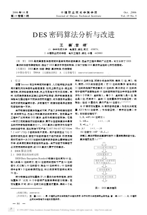
2 D ES 算法分析2.1 DES 算法的加密过程DES (Data Encryption Standard )数据分组长度为64位,输入的是64位的明文,在64位密钥的控制下产生64位的密文;反之输入64位的密文,输出64位的明文。

一种新的基于证据权重的D-S改进方法石闪闪【摘要】针对D-S证据理论处理高冲突证据时会出现于直觉相悖结论的问题,提出了一种基于证据权重组合的方法.首先通过引入Jousselme距离函数来确定证据权重.然后冲突证据由平均证据代替;且其权重也赋给平均证据.最后对修正后的证据加权平均后再用Dempster组合规则实现数据融合.与其他改进方法通过实例比较,表明该方法在有冲突证据时更能有效快速地识别出目标.【期刊名称】《科学技术与工程》【年(卷),期】2014(014)008【总页数】5页(P205-209)【关键词】组合规则;证据可信度;信息融合;目标识别【作者】石闪闪【作者单位】太原科技大学电子信息工程学院,太原030024【正文语种】中文【中图分类】TP181证据理论作为一种不确定性推理方法,近年来发展较大。
证据推理最初是由Dempster在1967年用多值映射得出了概率的上下界[1]而推出的;后来他的学生 Shafer进一步发展了该理论[2];因此又称为D-S理论。
其在不确定推理和数据融合领域应用广泛;但有些情况下,证据理论结果会与直觉相悖,为此各种解决方法被相继提出。
本文提出了一种新的有效处理冲突证据的方法,实验结果表明,该方法能得到更加直观合理的结果。
1 D-S的基本理论定义1 辨识框架:设有一个判决问题,所有可能结果的集合用Θ表示,Θ称为辨识框架。
定义2 基本概率赋值函数:设Θ为辨识框架,映射m:2Θ→[0,1](2Θ是Θ 的幂集)满足:则称m为Θ上的基本概率赋值函数,m(A)称为A的基本置信度,表示对A的精确信任。
定义3 D-S组合公式:设辨识框架Θ下两证据的 BPA(basic probability assignment)为 m1和m2,则D-S组合公式为:式(1)中,C ∈2Θ,Ai∈2Θ,Bj∈2Θ;而 k可以表示,称为证据之间的冲突概率。
2 D-S失效问题分析Dempster组合规则的优势不容置疑,但其在处理严重冲突证据时却存在失效问题。
ISE入门手册第一章ISE简介1.1关于ISE NEWS1.1.1 ISE CEO的话作为ISE的创立者和CEO,我很骄傲地展示我们地最新版本——ISE NEWS。
通过这个news字母,ISE的全体工作人员想告诉你我们公司的地位和新的发展计划,以便使你产生兴趣。
ISE优秀的性能和软件产品质量的显著增长、最好的技术支持、咨询服务是我们全体工作人员最好的礼物。
为了与这种增长相协调,截至2004年六月ISE的全体员工增加到100人左右。
在news这个版本中,我们提供了几个各领域中大家感兴趣的应用例子,比如:100nm以下CMOS和三维的非易失存储器结构的生成和网格剖分,垂直腔面发射激光器(VCSEL)的优化以及现代CMOS图像传感器的特性模拟。
VCSEL的部分由我们的客户和我们的研究咨询人员合作完成,是连接工业、学术和ISE一个成功的例子。
我相信你将喜欢这个news字母和它的内容。
为了得到进一步的信息,请访问我们的网站。
向大家表示最好的祝愿。
Wolfgang Fichtner1.1.2 ISE剧烈的增长路线通过对重要人力和资源的计划和投资考虑,将继续扩大ISE商业和利益。
从2001开始,在2002里有38%的增长,在2003年的进程中――ISE公司的十周年纪念日,ISE在网络规模中额外地增长了41%。
这种增长在2004年里将会继续下去,预期网络规模将增长35%。
咨询和客户工程服务已经是ISE最重要的发展部门。
这种有力的增长是以企业根基为基础。
除了在全球范围内赢得主要的新客户外,ISE正繁荣昌盛,因为长期支持ISE的客户反复地表示他们对ISE的忠诚和他们对ISE能力的信任,并表达了这种结果。
通过强有力的支持和ISE不断的培养强有力的商业关系,ISE努力使每一个客户得到满意。
图1.1 ISE集成系统的应用情况当今ISE已经成功进入光电子学市场。
除了ISE TCADTM软件引导客户的这种规模外,ISE可以在工业环境中毫无疑问地建立ISE光电子学的标准,另外一个强调的重点是满足CMOS传感器件压倒性的需求。
DE11043-LIs Your Autodesk CFD Analysis Accurate Or Could You Do Better?Jon WildeAutodeskLearning Objectives∙ A deeper insight into mesh requirements∙Learn about solver controls∙ A greater understanding of convergence∙Ability to achieve a higher level of results accuracyDescriptionThis class will include a competition to set up a model to achieve the best accuracy. It will begin with a discussion and hands-on session involving meshing—basic rules of meshing, mesh sensitivity, and mesh controls; solver settings—Advection Schemes, Nodal aspect ratio, Mach number, and Y+; convergence controls and interpretation; momentum conservation; and energy balance. Finally we will have a competition to apply what was discussed to produce an accurate simulation. Geometry and a description of the test environment will be provided, along with the results required. It is assumed that the user will have a good understanding of the software and can already set up his or her models to a good level.Your AU ExpertJon Wilde is a Senior Support Specialist at Autodesk supporting our Simulation products. He is also KDE for Simulation CFD.His main love and focus is CFD.Since graduating in 2003, he has worked with various analysis software, initially working within the defence sector, using structural (FEA) analysis while designing flight simulators, moving to both structural and thermal (CFD) analyses on airborne and maritime radomes.He then moved out of the defence industry and has focused solely on CFD ever since, working with Autodesk CFD for the last 8 years.His time now is spent supporting customers through 1:1 support and on our forums. He also helps in producing online content and running webinars (which are all recorded and published on YouTube).A deeper insight into mesh requirementsWhat is the definition of a good mesh?Ideally, results should be independent of mesh density. This means that if the mesh was refined, the results would not be affected.Often, if just using the automatic mesh sizing, this is not the case. By default, the CFD mesher uses edges to define the mesh sizing. This can mean that surfaces and volumes that have areas far from an edge, could be meshed coarser than they should be.It is also important to note that the mesher does not know the difference between a building or a valve. This means it does not know where or why a refined mesh is required. The user sometimes needs to add some intelligent meshing.This is an Automatic MeshdP = 0.397BarThis is a mesh that has undergone refinement. The difference in results demonstrates the huge effect that a change in mesh can have.dP = 0.230BarKnowing this, it is recommended that the user refines the mesh before beginning the solution. Some rules of thumb are to have:1. A fine enough mesh so that it accurately represents the CAD modela.If a cylinder in CAD looks like a hexagon once meshed in CFD – the results are going tobe comparable to flow through or around a hexagon rather than the intended smoothpipe2.Four to five elements through a small gap or channel as a minimuma.Ideally each gap should have enough elements to capture a flow gradient from a wall,through to the main flow region and back to the opposite wallb.The mesh enhancement (boundary layer) will also help with this but it needs a goodstarting point (See Y+ on p11 also)3.Surface and possibly Gap Refinement ona.Surface Refinement will mean that the mesh is no longer just controlled by edges butthat it is well distributed over surfaces alsob.When using the automated Gap Refinement, testing has shown that three elements isan optimum balance between accuracy and solution time4.The correct mesh through fans/blower/resistancesa.Meshed with a uniform mesh size to include four or five elements from the inlet tooutlet face5. A mesh sensitivity studyOther advanced functionality like Volume Growth Rate can also be enabled. This takes the mesh one level further by controlling the rate at which the mesh coarsens as it spreads out from edges and surfaces. The default is 1.35 (this means that adjacent elements can be no more than 35% different in size) and this can be lowered to ensure that the automatic mesh within a volume is finer than it otherwise might be.1. A fine enough mesh so that it accurately represents the CAD modelA fine mesh should capture the geometry well enough that differences are hard to spot. The coarse mesh here is clearly not representative of reality. As well as affecting the flow, it is also changing the flow results.The coarse mesh is causing the wheels to appear pentagonal.2.Four to five elements through a small gap or channel is a sensible minimumThis is a simple heat sink with a heat load beneath it.In each scenario, the mesh was refined further from the automatic mesh. The images below show the flow profile through the gaps between the fins of the heat sink as well as the temperature of the chip. It can be seen how the results improve as the mesh becomes finer.There are a few points to consider when meshing this model1.Capturing the flow profile through the gap2.Sufficient mesh through the inlet and outlet channels3.Having at least two elements through the thickness of a solid is also beneficial as it allows CFDto plot a thermal gradient. With just one element this is not possible. Again this can beautomated by using the ‘Thin Solid Elements’ option.With a heat sink, the fin temperature tends to be the same from one side to the other so this is not considered here.This is a comparison between the results of each of the scenarios.The images show the difference in mesh between two fins as it was refined.3.Surface and Gap Refinement OnThe model below was refined globally to 0.3 (so that there was sufficient mesh across the inlet and outletthicknesses) and with both Surface Refinement and Gap Refinement on. Notice thatthree gap elements were used.What this demonstrates is that using the advanced meshing tools in CFD, the mesh through small gaps is properly captured with minimal effort. This is a great way to begin an adaptive mesh cycle.Temperature ComparisonThis shows the maximum chip temperature between each of the designs.4.The correct mesh through fans/blower/resistancesThese images are to demonstrate what can happen if the mesh is insufficient. What will typically be found is that the flow rate and/or pressure drop are incorrectly predicted.With a poor mesh and if a fan curve or head capacity curve were assigned, it is possible that the item could operate at a point off of the curve, which is not realistic.5.Mesh Sensitivity StudyRunning a manual study can be a quick way to verify that the results are independent of the mesh.To do this:∙Pick some critical values from the results of the studyo Making these summary points/parts is useful at this stage∙Clone the scenario∙Refine the mesh by 30% (select everything and refine to 0.7)∙Compare the results between scenarios (utilize the Decision Centre)∙If the results vary by less than 5%, it is safe to assume that the results of the previous study were independent of the mesh settings. If not, repeat the process until this is achievedUsers might utilise Adaptive Meshing based off of an initial automatically sized mesh. This is not recommended.Instead, apply the above settings as a starting point and allow CFD to automatically refine the mesh further once a converged solution is obtained.Solver ControlsAdvection SchemesAdvection is the numerical mechanism of transporting a quantity (velocity, temperature, etc.) through the solution domain. There are five options available within CFD.∙Advection Scheme 1o Used to be the workhorse and is still the default but is now superseded by ADV5 for almost everything except:▪Surface Resistances (inaccuracy with other ADV schemes)▪Free Surface Analyses (where ADV1 is the default setting) ∙Advection Scheme 2o Rarely used (ADV5 has superseded this entirely)∙Advection Scheme 3o Rarely used. It used to be used for external aerodynamics but again, ADV5 tends to be better∙Advection Scheme 4o Long skinny ducts∙Advection Scheme 5o The new kingo Recommended for almost all types of analyses and turbulence models. If in doubt though, log a case and request some assistance from our engineersTurbulence ModelsThere are many options here although typically one or two are suitable for almost all applications.The default is k-epsilon and works well for most studies.The other that is becoming more common now (since it has recently been added to Autodesk CFD) is SST –k-omega. We might change to this when looking at external aerodynamics, if we have problems with predicting internal pressure drop or are struggling to properly capture a thermal gradient at the wall.For natural convection models, we might also utilize the Mixing Length model, which seems to produce more accurate results and often in a shorter time than other models.Intelligent Wall FormationThis is enabled automatically if SST is enabled.It is often wise to enable this for the k-epsilon model if refining the mesh. It means that the sensitivity to the Y+ value is removed, which can be useful if this value drops below 35.Results QuantitiesThere are some very useful values within this window and they are off by default. To access these options:And to turn on the three shown here, which will be discussed below:Mach Number∙If the analysis is compressible and the user was unaware, the set up will almost certainly be wrongo Values above 0.3 are subsonic and might show some compressibilityo Values above 0.7 are likely to contain the beginnings of shockwaves – these need to be run compressible∙If the Mach number is showing that an analysis is not solely incompressible, a different setup will be needed. The online CFD help is useful here but so might be logging a support request for model verificationY+∙This can be a really useful tool to identify mesh quality and the required value will vary depending on the chosen turbulence model, As an example for the two most commonly usedmodels in Autodesk CFD:o SST Y+ < 1o ke 35 < Y+ < 300Stream Function∙This will enable Nodal Aspect Ratio (NAR), which is the ratio of the longest to shortest edge of any single element. This is an indication of how equilateral or skewed each element is. Thecloser to 1 this value is, the more equilateral the element and the better the mesh quality o The lower the NAR, the more accurate the analysis tends to beo The ideal scenario is to have most elements beneath an NAR of 100-150▪It is acceptable to have the NAR up to 500,000 in regions that are of no interest to the user, although this is likely to increase the time taken to solve an analysis ▪If the NAR is close to 1, CFD will use closer to 1GB of RAM for each millionelements. This will be closer to 2.5 GB for most meshesThis is an element with a NAR of 1:This is an element with a NAR of 50 (still acceptable)Imagine an element with an NAR of 1000 (this is very skewed. Picture this capturing flow through a narrow path – it would not produce an accurate representation of reality).Using NAR can be a hugely useful tool if the meshing fails during volumetric meshing or the optimizing stage.Often, CFD is unable to create the boundary layer due to a small gap or angle in the model. If two inward facing boundary layers overlap, the mesher will run into issues.To identify where this is occurring:∙Turn off Mesh Enhancement (so there will be no boundary layer created)∙Mesh the model (no need to run any iterations, just generate the mesh)∙Plot NAR as an ISO surfaceo Typically there will be regions of high NAR and these are often where small gaps or infinite angles exist within the fluid. Infinite angles can occur if a radii meets a planarsurface. This kind of shape is difficult to mesh with tetrahedrons∙Return to CAD and close up gaps and/or remove infinite angles from in the fluid (where an fillet meets a planar surface is a good example of this)o Alternatively, the mesh on small surfaces can be refined but this is only recommended if these regions are realistic. Taking a short-cut here just to get a mesh is unwise as therun time with a poor mesh will usually take longer than fixing the CAD and can still leavethe user with poor resultso As we know from before, the higher the NAR, the more RAM is required to mesh the model and typically the longer the run timeA greater understanding of convergenceAdjusting the Convergence CriteriaSometimes, CFD stops at a solution before the analysis is truly converged.This can happen if there are very minor changes between iterations or during a transient analysis. A finer mesh will almost certainly mean that less changes from one iteration to the next, so in a drive for a more accurate solution, one must also consider the convergence criteria.Generally, changing this from the default to a ‘Tight’ setting is sufficient. Although it is also acceptable to manually tweak the convergence values further still. A further factor of ten is what is usually used if very tight convergence is required, although the model could run for a very long time with this setting.There are additional controls here that can help to smooth convergence but will also slow the solution process.Ability to achieve a higher level of results accuracyMomentum ConservationIt is possible that due to a few factors, the flow entering the model does not equal the flow exiting. This can be verified by using the bulk calculator. Although CFD can stop and proclaim convergence once there is minimal change between iterations, it is sensible to check that the flow is entering and leaving as expected.The most common issue here is that the outlet extensions are too short, causing recirculation over what is typically a P=0. Simply assigning a velocity at the outlet and a pressure at the inlet to work around this is not a practical solution as the analysis will still be chopping off part of what is happening in reality.A solution is to add outlet extensions to the CAD model. These tend to be ten times their diameter (or width) in length and should allow the completion of any recirculation before the flow exits the model. If this recirculation is not completed or occurs over the outlet, the pressure drop through the system will likely not be accurate. Refer back to the image on p5 for an example of this.An easy way to see if this is occurring is to add Global Vectors to the model. These always originate at inlets and outlets (and fans/resistances). They should help the user to quickly understand if the flow is exiting the outlets smoothly or if there is recirculation.It is also to extend the inlet extrusions to about five times the diameter (or width) of the duct. This helps flow become more developed before entering the region under scrutiny. Without this, we could end up with a poor result. If there are suppressed air ducts, pumping flow to an internal section of the model – recess the inlet boundary conditions a little inside the ducts to allow the flow to develop before entering the room, just like a standard inlet.Energy BalanceIf flow is re-entering the outlet, CFD is not going to be able to predict what temperature it should be and therefore there will be a poor energy balance. Although it is likely divergence will occur here, it is possible that the model could converge with a poor thermal balance, or at least a poor thermal solution. Utilise the Summary File (.sol). It details how much energy is entering and leaving the model. This is a great starting point for validating the energy balance of a model.This is taken from the Summary file and shows the Energy Out – Energy In value is small (close to zero is expected).It is also useful to check that any energy we know was inputted to the model has been captured and passed to the fluid domain.The combination of all of these factors should yield improved results accuracy.In reality, all need to be carefully considered during a CFD project.。
以前的SolidWorks Simulation(COSMOS Works)中有一个很好的功能-设计情形,此功能能够快速的对范围值进行系列分析,分析对比出不同的数值时,结果的差异.在SolidWorks 2010中,此功能被设计算例替代下面以一个小例子演示其过程:1 分析流程设计算例的分析流程图如下:根据其流程图,其分析过程大致如下:首先建立一个模拟算例,然后添加一个设计算例,在设计算例中,定义各个变量条件,然后在模拟算例中关联设计算例的变量条件。
然后在设计算例中,定义约束与设计结果的目标,如果需要优化,请点选优化。
2 实例演示打开SolidWorks Simulation在线指导教程->静态指导教程->零件分析中的默认的静态实例Tutor1.SLD PRT。
在(默认在安装目录的SolidWorks文件夹下的Simulation文件夹下的Examples文件夹下:如示例路径:C:\Program Files\SolidWorks Corp 2010 SP3.1\SolidWorks\Simulation\Examples\ )2.1 定义模拟算例按照在线指导教程教程中的设置,定义所有的设置过程,定义完毕如下:2.2 增加一个设计算例(假设分析1000PSI 2000PSI 和3000PSI下零件的受力)增加一个变量2.3 将变量值与模拟算例相关联打开模拟算例的外观载荷,右键编辑定义在数值框一栏点链接数值选择刚才定义的变量,点确定。
这样变量就与模拟算例产生了关联。
2.4 增加一个目标(即分析结果需求)假设我们相比较位移值2.5 在表格视图中增加设计情形2.6 点运行3 结果可以设置多个参数(载荷、约束、尺寸等等)通过情形,进行配置,减少人工机械性重复的设置、以更快、更简洁的得到更好的设计结果。
ADSPA仿真负载牵引心得加入ADS 群半年多来,不时在群里面碰到有人问做负载牵引时出现的不收敛问题,虽然自己也自告奋勇的出来聊几句,奈何自己的文采有限,无法说清楚这个问题。
其实我自己半年前也曾为此问题困扰一个星期之久,幸好有群里面的流星和羽纤二位大哥的指点,二位大哥对我在ADS 操作和射频微波功放方面的困惑进行了无私的指点,加快了我完成了雷达发射机的研制进程,对此我深表感谢。
前些时候,群里面部分同样如我半年前一样在负载牵引上遇到困惑的人邀请我写一个实例,用这个实例来说明如何解决负载牵引中碰到的不收敛问题,由于这几天我刚接手了另外两个雷达发射机的研制项目,一直没有抽出足够的时间来写,今天有时间就做个注解,写得不好,不要介意,但愿本文档对一些刚入门的新手在碰到负载牵引时出现的不收敛问题能提供一些帮助。
下面我以freescale的新一代功放管MRF6V2300作为例子来说明负载牵引问题。
MRF6V2300 是freescale 推出的新一代功放管,CW 输出功率为300W,额定漏工作电压为50V,工作频率为10-600MHz,价格仅500 元一只,是米波雷达和广播电视发射机的廉价实用管子。
其DATASHEET 上提供了三个典型的频率点的输入和输出阻抗:27MHz,220MHz,450MHz。
参考静态偏置电压典型值为2.6V时,其静态偏置电流典型值是900mA,因为比较容易,这里面我不作静态电流的仿真了,直接采用静态偏置电压2.6V(ADS仿真结果是919mA)。
先仿真频点f1=27MHz,datasheet 上显示其输出负载Zload=3.50+j*0.19。
我们打开ADS,新建一个空白原理图,在其工具栏的DesignGuide上点击下拉菜单中选择Amplifier 点1-Tone Nonlinear Simulations 展开,选择Load-Pull-PAE,Output Power Contours 然后点击OK按钮就行了,出来如图1-1 所示的原始原理图和图1-2 所示的原始仿真图:图1-1 Load-Pull 原始原理图图1-2 Load-Pull 原始仿真图对图1-1,我们首先更换管子成我们要测试的MRF6V2300N,把两个图标都换上,然后输入功率Pavs 改成20dBm,频率RF freq 改成27MHz,漏电压Vhigh改成50,栅压(偏置电压)改成2.6,其它都不变,如图1-3 所示:图1-3 更换成MRF2300N后的原理图这里面输入功率之所以选择20dBm 是因为在这么的频率,其输入输出阻抗都比较大,其增益很高,稍微大点其输出就饱和了,有可能会导致不收敛,不利于以后的调整,接着点仿真按钮,结果如图1-4 所示:图1-4 换成MRF6V2300N后的仿真图从图1-4 可以看到,在输入为20dBm的情况下,其输出已经达到了53.79dBm了,这离其典型输出功率300W(54.7dBm)已经很接近,但我们从图1-4 的左下角的坐标图中看到其功率圆和效率圆的圆心都没有显示出来,对图1-4左下角的坐标图局部放大如图1-5所示:图1-5 左下角坐标图局部放大图从图1-5 中,我们可以看出,其功率圆和效率圆的圆心在图的正左方,我们重新设定图1-1 中原始图的圆心,我们大胆猜测其圆心s11_center 为-0.75+j*0.0,半径s11_rho 为0.2,并将采样点数改为500,如图1-6 所示:图1-6 重新设置圆心和采样点数为何半径要设置成0.2 呢?而不是0.3 或者更大呢?大点不是好吗?半径大点能把所有可能的情况都仿真进去,何乐而不为呢?不行!因为要撑破的!一个原则是你仿真的范围不能超过1!也就是你坐标圆的圆心加半径不能超过1!为保险起见,二者之和最大为0.99!也就是说:个人喜欢两者之和为0.99,因为某些管子输出功率很大,其输入输出阻抗很小,不到0.99 功率圆和效率圆可能没出来!如本例,如果半径是0.3 的话,就不收敛了!为何采样点数为500?这个···那个···纯属个人喜好,如果你喜好,你也可以改成1000,不过这样你的电脑反应速度就慢了,电脑差点,单核的话可能要花好几分钟时间。