PhysRevLett[1].86.3188

Physica A 374(2007)483–490Identification of overlapping community structure in complexnetworks using fuzzy c -means clusteringShihua Zhang a,Ã,Rui-Sheng Wang b ,Xiang-Sun Zhang aa Academy of Mathematics &Systems Science,Chinese Academy of Science,Beijing 100080,Chinab School of Information,Renmin University of China,Beijing 100872,ChinaReceived 28June 2006Available online 7August 2006AbstractIdentification of (overlapping)communities/clusters in a complex network is a general problem in data mining of network data sets.In this paper,we devise a novel algorithm to identify overlapping communities in complex networks by the combination of a new modularity function based on generalizing NG’s Q function,an approximation mapping of network nodes into Euclidean space and fuzzy c -means clustering.Experimental results indicate that the new algorithm is efficient at detecting both good clusterings and the appropriate number of clusters.r 2006Elsevier B.V.All rights reserved.Keywords:Overlapping community structure;Modular function;Spectral mapping;Fuzzy c -means clustering;Complex network1.IntroductionLarge complex networks representing relationships among set of entities have been one of the focuses of interest of scientists in many fields in the recent years.Various complex network examples include social network,worldwide web network,telecommunication network and biological network.One of the key problems in the field is ‘How to describe/explain its community structure’.Generally,a community in a network is a subgraph whose nodes are densely connected within itself but sparsely connected with the rest of the network.Many studies have verified the community/modularity structure of various complex networks such as protein-protein interaction network,worldwide web network and co-author network.Clearly,the ability to detect community structure in a network has important practical applications and can help us understand the network system.Although the notion of community structure is straightforward,construction of an efficient algorithm for identification of the community structure in a complex network is highly nontrivial.A number of algorithms for detecting the communities have been developed in various fields (for a recent review see Ref.[1]and a recent comparison paper see Ref.[2]).There are two main difficulties in detecting community structure.The first is that we don’t know how many communities there are in a given network.The usual drawback in many /locate/physa0378-4371/$-see front matter r 2006Elsevier B.V.All rights reserved.doi:10.1016/j.physa.2006.07.023ÃCorresponding author.E-mail addresses:zsh@ (S.Zhang),wrs@ (R.-S.Wang),zxs@ (X.-S.Zhang).algorithms is that they cannot give a valid criterion for measuring the community structure.Secondly,it is a common case that some nodes in a network can belong to more than one community.This means the overlapping community structure in complex networks.Overlapping nodes may play a special role in a complex network system.Most known algorithms such as divisive algorithm [3–5]cannot detect them.Only a few community-detecting methods [6,7]can uncover the overlapping community structure.Taking into account the first difficulty,Newman and Girvan [8]has developed a new approach.They introduced a modularity function Q for measuring community structure.In order to write the context properly,we refer to a similar formulation in Ref.[5].In detail,given an undirected graph/network G ðV ;E ;W Þconsisting of the node set V ,the edge set E and a symmetric weight matrix W ¼½w ij n Ân ,where w ij X 0and n is the size of the network,the modularity function Q is defined asQ ðP k Þ¼X k c ¼1L ðV c ;V c ÞL ðV ;V ÞÀL ðV c ;V ÞL ðV ;V Þ 2"#,(1)where P k is a partition of the nodes into k groups and L ðV 0;V 00Þ¼P i 2V 0;j 2V 00w ði ;j Þ.The Q function measuresthe quality of a given community structure organization of a network and can be used to automatically select the optimal number of communities k according to the maximum Q value [8,5].The measure has been used for developing new detection algorithms such as Refs.[5,9,4].White and Smyth [5]showed that optimizing the Q function can be reformulated as a spectral relaxation problem and proposed two spectral clustering algorithms that seek to maximize Q .In this study,we develop an algorithm for detecting overlapping community structure.The algorithm combines the idea of modularity function Q [8],spectral relaxation [5]and fuzzy c -means clustering method[10]which is inspired by the general concept of fuzzy geometric clustering.The fuzzy clustering methods don’t employ hard assignment,while only assign a membership degree u ij to every node v i with respect to the cluster C j .2.MethodSimulation across a wide variety of simulated and real world networks showed that large Q values are correlated with better network clusterings [8].Then maximizing the Q function can obtain final ‘optimal’community structure.It is noted that in many complex networks,some nodes may belong to more than one community.The divisive algorithms based on maximizing the Q function fail to detect such case.Fig.1shows an example of a simple network which visually suggests three clusters and classifying node 5(or node 9)intoFig.1.An example of network showing Q and e Qvalues for different number k of clusters using the same spectral mapping but different cluster methods,i.e.k -means and fuzzy c -means,respectively.For the latter,it shows every node’s soft assignment and membership of final clusters with l ¼0:15.S.Zhang et al./Physica A 374(2007)483–490484two clusters at the same time may be more appropriate intuitively.So we introduce the concept of fuzzy membership degree to the network clustering problem in the following subsection.2.1.A new modular functionIf there are k communities in total,we define a corresponding n Âk ‘soft assignment’matrix U k ¼½u 1;...;u k with 0p u ic p 1for each c ¼1;...;k and P kc ¼1u ic ¼1for each i ¼1;...;n .With this we define the membership of each community as ¯V c ¼f i j u ic 4l ;i 2V g ,where l is a threshold that can convert a soft assignment into final clustering.We define a new modularity function e Q as e Q ðU k Þ¼X k c ¼1A ð¯V c ;¯V c ÞA ðV ;V ÞÀA ð¯V c ;V ÞA ðV ;V Þ 2"#,(2)where U k is a fuzzy partition of the vertices into k groups and A ð¯V c ;¯V c Þ¼P i 2¯V c ;j 2¯V c ððu ic þu jc Þ=2Þw ði ;j Þ,A ð¯V c ;V Þ¼A ð¯V c ;¯V c ÞþP i 2¯V c ;j 2V n ¯V c ððu ic þð1Àu jc ÞÞ=2Þw ði ;j Þand A ðV ;V Þ¼P i 2V ;j 2V w ði ;j Þ.This of coursecan be thought as a generalization of the Newman’s Q function.Our objective is to compute a soft assignment matrix by maximizing the new Q function with appropriate k .How could we do?2.2.Spectral mappingWhite and Smyth [5]showed that the problem of maximizing the modularity function Q can be reformulated as an eigenvector problem and devised two spectral clustering algorithms.Their algorithms are similar in spirit to a class of spectral clustering methods which map data points into Euclidean space by eigendecomposing a related matrix and then grouping them by general clustering methods such as k -means and hierarchical clustering [5,9].Given a network and its adjacent matrix A ¼ða ij Þn Ân and a diagonal matrix D ¼ðd ii Þ,d ii ¼P k a ik ,two matrices D À1=2AD À1=2and D À1A are often used.A recent modification [11]uses the top K eigenvectors of the generalized eigensystem Ax ¼tDx instead of the K eigenvectors of the two matrices mentioned above to form a matrix whose rows correspond to original data points.The authors show that after normalizing the rows using Euclidean norm,their eigenvectors are mathematically identical and emphasize that this is a numerically more stable method.Although their result is designed to cluster real-valued points[11,12],it is also appropriate for network clustering.So in this study,we compute the top k À1eigenvectors of the eigensystem to form a ðk À1Þ-dimensional embedding of the graph into Euclidean space and use ‘soft-assignment’geometric clustering on this embedding to generate a clustering U k (k is the expected number of clusters).2.3.Fuzzy c-meansHere,in order to realize our ‘soft assignment’,we introduce fuzzy c -means (FCM)clustering method [10,13]to cluster these points and maximize the e Qfunction.Fuzzy c -means is a method of clustering which allows one piece of data to belong to two or more clusters.This method (developed by Dunn in 1973[10]and improved by Bezdek in 1981[13])is frequently used in pattern recognition.It is based on minimization of the following objective functionJ m ¼Xn i ¼1X k j ¼1u m ij k x i Àc j k 2,(3)over variables u ij and c with P j u ij ¼1.m 2½1;1Þis a weight exponent controlling the degree of fuzzification.u ij is the membership degree of x i in the cluster j .x i is the i th d -dimensional measured data point.c j is the d -dimensional center of the cluster j ,and k Ãk is any norm expressing the similarity between any measured data and the center.Fuzzy partitioning is carried out through an iterative optimization of the objective function shown above,with the update of membership degree u ij and the cluster centers c j .This procedure converges to a local minimum or a saddle point of J m .S.Zhang et al./Physica A 374(2007)483–4904852.4.The flow of the algorithmGiven an upper bound K of the number of clusters and the adjacent matrix A ¼ða ij Þn Ân of a network.The detailed algorithm is stated straightforward for a given l as follows:Spectral mapping:(i)Compute the diagonal matrix D ¼ðd ii Þ,where d ii ¼P k a ik .(ii)Form the eigenvector matrix E K ¼½e 1;e 2;...;e K by computing the top K eigenvectors of thegeneralized eigensystem Ax ¼tDx .Fuzzy c -means:for each value of k ,2p k p K :(i)Form the matrix E k ¼½e 2;e 3;...;e k from the matrix E K .(ii)Normalize the rows of E k to unit length using Euclidean distance norm.(iii)Cluster the row vectors of E k using fuzzy c -means or any other fuzzy clustering method to obtain a softassignment matrix U k .Maximizing the modular function:Pick the k and the corresponding fuzzy partition U k that maximizes e QðU k Þ.In the algorithm above,we initialize FCM such that the starting centroids are chosen to be as orthogonal as possible which is suggested for k -means clustering method in Ref.[12].The initialization does not change the time complexity,and also can improve the quality of the clusterings,thus at the same time reduces the need for restarting the random initialization process.The framework of our algorithm is similar to several spectral clustering methods in previous studies[5,9,12,11].We also map data points (work nodes in our study)into Euclidean space by computing the top K eigenvectors of a generalized eigen system and then cluster the embedding using a fuzzy clustering method just as others using geometric clustering algorithm or general hierarchical clustering algorithm.Here,we emphasize two key points different from those earlier studies:We introduce a generalized modular function e Q employing fuzzy concept,which is devised for evaluating the goodness of overlapping community structure. In combination with the novel e Qfunction,we introduce fuzzy clustering method into network clustering instead of general hard clustering methods.This means that our algorithm can uncover overlapping clusters,whereas general framework:‘‘Objective function such as Q function and Normalized cut function+Spectral mapping+general geometric clustering/hierarchical clustering’’cannot achieve this.3.Experimental resultsWe have implemented the proposed algorithm by Matlab.And the fuzzy clustering toolbox [14]is used for our analysis.In order to make an intuitive comparison,we also compute the hard clustering based on the original Q -function,spectral mapping (same as we used)and k -means clustering.We illustrate the fuzzy concept and the difference of our method with traditional divisive algorithms by a simple example shown in Fig.1.Just as mentioned above,the network visually suggests three clusters.But classifying node 5(or node 9)simultaneously into two clusters may be more reasonable.We can see from Fig.1that our method did uncover the overlapping communities for this simple network,while the traditional method can only make one node belong to a single cluster.We also present the analysis of two real networks,i.e.the Zachary’s karate club network and the American college football team network for better understanding the differences between our method and traditional methods.S.Zhang et al./Physica A 374(2007)483–490486S.Zhang et al./Physica A374(2007)483–490487 3.1.Zachary’s karate clubThe famous karate club network analyzed by Zachary[15]is widely used as a test example for methods of detecting communities in complex networks[1,8,16,3,4,17,9,18,19].The network consists of34members of a karate club as nodes and78edges representing friendship between members of the club which was observed over a period of two years.Due to a disagreement between the club’s administrator and the club’s instructor, the club split into two smaller ones.The question we concern is that if we can uncover the potential behavior of the network,detect the two communities or multiple groups,and particularly identify which community a node belongs to.The network is presented in Fig.2,where the squares and the circles label the members of the two groups.The results of k-means and our analysis are illustrated in Fig.3.The k-means combined with Q function divides the network into three parts(see in Fig.3A),but we can see that some nodes in one cluster are also connected densely with another cluster such as node9and31in cluster 1densely connecting with cluster2,and node1in cluster2with cluster3.Fig.3B shows the results of our method,from which we can see that node1,9,10,31belong to two clusters at the same time.These nodes in the network link evenly with two clusters.Another thing is that the two methods both uncover three communities but not two.There is a small community included in the instructor’s faction,since the set of nodes5,6,7,11,17only connects with node1in the instructor’s faction.Note that our method also classifies node1into the small community,while k-means does not.work of American college football teamsThe second network we have investigated is the college football network which represents the game schedule of the2000season of Division I of the US college football league.The nodes in the network represent the115 teams,while the links represent613games played in the course of the year.The teams are divided into conferences of8–12teams each and generally games are more frequent between members of the same conference than between teams of different conferences.The natural community structure in the network makes it a commonly used workbench for community-detecting algorithm testing[3,5,7].Fig.4shows how the modularity Q and e Q vary with k with respect to k-means and our method,respectively. The peak for k-means is at k¼12,Q¼0:5398,while for our algorithm at k¼10,e Q¼0:4673with l¼0:10. Both methods identify ten communities which contain ten conferences almost exactly.Only teams labeled as Sunbelt are not recognized as belonging to a same community for both methods.This group is classified as well in the results of Refs.[3,19].This happens because the Sunbelt teams played nearly as many games against Western Athletic teams as they played in their own conference,and they also played quite a number of gamesagainst Mid-American team.Our method identified11nodes(teams)which belong to at least twoFig.2.Zachary’s karate club network.Square nodes and circle nodes represent the instructor’s faction and the administrator’s faction, respectively.Thisfigure is from Newman and Girvan[8].communities (see Fig.5,11red nodes).These nodes generally connect evenly with more than one community,so we cannot classify them into one specific community correctly.These nodes represent ‘fuzzy’points which cannot be classified correctly by employing current link information.Maybe such points play a ‘bridge’role in two or more communities in complex network of other types.4.Conclusion and discussionIn this paper,we present a new method to identify the community structure in complex networks with a fuzzy concept.The method combines a generalized modularity function,spectral mapping,and fuzzy clustering technique.The nodes of the network are projected into d -dimensional Euclidean space which is obtained by computing the top d nontrivial eigenvectors of the generalized eigensystem Ax ¼tDx .Then the fuzzy c -means clustering method is introduced into the d -dimensional space based on general Euclidean distance to cluster the data points.By maximizing the generalized modular function e QðU d Þfor varying d ,we obtain the appropriate number of clusters.The final soft assignment matrix determines the final clusters’membership with a designated threshold l .Fig.3.The results of both k -means and our method applied to karate club network.A:The different colors represent three different communities obtained by k -means and the right table shows values of NG’Q versus different k .B:Four red nodes represent the overlap of two adjacent communities obtained by our method and the right table shows values of new Q versus different k with l ¼0:25.3.t y 0510152000.10.20.30.40.50.6k-meansK N G ' Q 0510152000.10.20.30.40.5fuzzy c-means K N e w Q Fig.4.Q and e Qvalues versus k with respect to k -means and fuzzy c -means clustering methods for the network of American college football team.S.Zhang et al./Physica A 374(2007)483–490488Although spectral mapping has been comprehensively used before to detect communities in complex networks (even in clustering the real-valued points),we believe that our method represents a step forward in this field.A fuzzy method is introduced naturally with the generalized modular function and fuzzy c -means clustering technique.As our tests have suggested,it is very natural that some nodes should belong to more than one community.These nodes may play a special role in a complex network system.For example,in a biological network such as protein interaction network,one node (protein or gene)belonging to two functional modules may act as a bridge between them which transfers biological information or acts as multiple functional units [6].One thing should be noted is that when this method is applied to large complex networks,computational complexity is a key problem.Fortunately,some fast techniques for solving eigensystem have been developed[20]and several methods of FCM acceleration can also be found in the literature [21].For instance,if we adopt the implicitly restarted Lanczos method (IRLM)[20]to compute the K À1eigenvectors and the efficient implementation of the FCM algorithm in Ref.[21],we can have the worse-case complexity of O ðmKh þnK 2h þK 3h Þand O ðnK 2Þ,respectively,where m is the number of edges in the network and h is the number of iteration required until convergence.For large sparse networks where m $n ,and K 5n ,the algorithms will scale roughly linearly as a function of the number of nodes n .Nonetheless,the eigenvector computation is still the most computationally expensive step of the method.We expect that this new method will be employed with promising results in the detection of communities in complex networks.AcknowledgmentsThis work is partly supported by Important Research Direction Project of CAS ‘‘Some Important Problem in Bioinformatics’’,National Natural Science Foundation of China under Grant No.10471141.The authors thank Professor M.E.J.Newman for providing the data of karate club network and the college football team network.Fig.5.Fuzzy communities of American college football team network (k ¼10and e Q¼0:4673)with given l ¼0:10(best viewed in color).S.Zhang et al./Physica A 374(2007)483–490489References[1]M.E.J.Newman,Detecting community structure in networks,Eur.Phys.J.B 38(2004)321–330.[2]L.Danon,J.Duch,A.Diaz-Guilera,A.Arenas,Comparing community structure identification,J.Stat.Mech.P09008(2005).[3]M.Girvan,M.E.J.Newman,Community structure in social and biological networks,A 99(12)(2002)7821–7826.[4]J.Duch,A.Arenas,Community detection in complex networks using extremal optimization,Phys.Rev.E 72(2005)027104.[5]S.White,P.Smyth,A spectral clustering approach to finding communities in graphs,SIAM International Conference on DataMining,2005.[6]G.Palla,I.Derenyi,I.Farkas,T.Vicsek,Uncovering the overlapping community structure of complex networks in nature and society,Nature 435(2005)814–818.[7]J.Reichardt,S.Bornholdt,Detecting fuzzy community structures in complex networks with a Potts model,Phys.Rev.Lett.93(2004)218701.[8]M.E.J.Newman,M.Girvan,Finding and evaluating community structure in networks,Phys.Rev.E 69(2004)026113.[9]L.Donetti,M.A.Mun oz,Detecting network communities:a new systematic and efficient algorithm,J.Stat.Mech.P10012(2004).[10]J.C.Dunn,A fuzzy relative of the ISODATA process and its use in detecting compact well-separated clusters,J.Cybernet.3(1973)32–57.[11]D.Verma,M.Meila,A comparison of spectral clustering algorithms.Technical Report,2003,UW CSE Technical Report 03-05-01.[12]A.Ng,M.Jordan,Y.Weiss,On spectral clustering:analysis and an algorithm,Adv.Neural Inf.Process.Systems 14(2002)849–856.[13]J.C.Bezdek,Pattern Recognition with Fuzzy Objective Function Algorithms,Plenum Press,New York,1981.[14]Fuzzy Clustering Toolbox-h http://www.fmt.vein.hu/softcomp/fclusttoolbox/i .[15]W.W.Zachary,An information flow model for conflict and fission in small groups,J.Anthropol.Res.33(1977)452–473.[16]M.E.J.Newman,Fast algorithm for detecting community structure in networks,Phys.Rev.E 69(2004)066133.[17]F.Radicchi,C.Castellano,F.Cecconi,V.Loreto,D.Parisi,Defining and identifying communities in networks,Proc.Natl.Acad.A 101(9)(2004)2658–2663.[18]F.Wu,B.A.Huberman,Finding communities in linear time:a physics approach,Eur.Phys.J.B 38(2004)331–338.[19]S.Fortunato,tora,M.Marchiori,A method to find community structures based on information centrality,Phys.Rev.E 70(2004)056104.[20]Z.Bai,J.Demmel,J.Dongarra,A.Ruhe,H.Vorst (Eds.),Templates for the Solution of Algebraic Eigenvalue Problems:A PracticalGuide,SIAM,Philadelphia,PA,2000.[21]J.F.Kelen,T.Hutcheson,Reducing the time complexity of the fuzzy c -means algorithm,IEEE Trans.Fuzzy Systems 10(2)(2002)263–267.S.Zhang et al./Physica A 374(2007)483–490490。

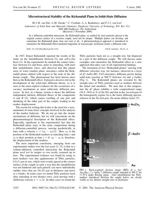
Microstructural Stability of the Kirkendall Plane in Solid-State Diffusion M.J.H.van Dal,A.M.Gusak,*C.Cserháti,A.A.Kodentsov,and F.J.J.van Loo†Laboratory of Solid State and Materials Chemistry,Einghoven University of Technology,P.O.Box513,5600MB Eindhoven,The Netherlands(Received3November2000)In a diffusion-controlled interaction,the Kirkendall plane,as marked by inert particles placed at the original contact surface of a reaction couple,need not be unique.Multiple planes can develop,and sometimes the Kirkendall plane does not exist at all.A phenomenological approach is introduced to rationalize the Kirkendall-effect-mediated migration of macroscopic inclusions inside a diffusion zone. DOI:10.1103/PhysRevLett.86.3352PACS numbers:66.30.–hIn1947,Ernest Kirkendall reported the results of hisstudy on the interdiffusion between Cu and a͑Cu,Zn͒brass[1].In his experiments he marked the contact inter-face between Cu and brass,prior to annealing,with inertthin molybdenum wires,and observed that this planararray of wires(marker plane,nowadays called the Kirk-endall plane)shifted with respect to the ends of the dif-fusion couple.This phenomenon has been known sincethen as the Kirkendall effect.It played a decisive role in thedevelopment of the solid-state diffusion theory,as it isseen as the most explicit evidence for the occurrence of avacancy mechanism in most solid-state diffusion pro-cesses.In fact,in a binary system it shows the differentindependent intrinsic diffusionfluxes of the componentsA and B[2],which causes swelling of one part and shrinking of the other part of the couple,leading to themarker displacement.The reason for writing this Letter is the need for a reex-amination of some basic concepts involved in the analysisof the marker behavior.We do not go into the atomicmechanisms of diffusion,but we will concentrate on thephenomenological description of the Kirkendall effect.Especially significant is the experimental fact that theKirkendall plane stays at the same composition duringa diffusion-controlled process,moving parabolically intime with a velocity y෇͑x K2x0͒͞2t.Here x K is the position of the Kirkendall markers at annealing time t andx0is their position at time t෇0;x K2x0is,therefore,the displacement of the markers.The most important conclusion,emerging from ourexperimental studies over the last years[3–5],is that in avolume-diffusion controlled interaction the Kirkendallplane need not be unique as was tacitly assumed up tonow.The experimental evidence was found by using asinert markers veryfine agglomerates of ThO2particles,0.55m m in size,which were evenly spread at the contactsurface of the couple in such a way that the interdiffusionwas not hindered and each particle can move individually(unlike wires that are1025m m in thickness and moveas a whole).In some cases we found ThO2particles backafter annealing in two distinct rows,each moving with a(different)velocity y෇x͞2t.In other cases we found the ThO2particles back not as a straight row,but dispersed in a part of the diffusion couple.We will discuss some examples and rationalize the Kirkendall effect in a new approach that takes care of all experimentalfindings. The formation of two“Kirkendall planes”moving with different velocities was,for instance,observed in a layer of b0-AuZn(B2;CsCl-structure),diffusion grown during solid-state reaction at500±C between Au and g-AuZn2 (Fig.1).The Kirkendall planes are revealed by the straight rows of ThO2particles used as markers between the initial end members.We note that at this tempera-ture the b0phase exhibits a wide compositional range (38.5–56.0at.%of Zn[6])and that in the Au-rich part of the homogeneity region Au is the faster diffusing species, whereas in the Zn-rich part,Zn-atoms diffuse faster[7].FIG.1.Back-scattered electron image(BEI)of a Au͞Au36Zn64(“g-AuZn2”)diffusion couple annealed at500±C for 17.25h underflowing argon.After interdiffusion the ThO2 markers introduced between the couple halves are clearly visible as two distinct straight rows of inclusions.33520031-9007͞01͞86(15)͞3352(4)$15.00©2001The American Physical SocietyThe appearance of more than one Kirkendall plane is not restricted to interdiffusion zones composed of a single-phased reaction product.For instance,Fig.2(a)shows a multiphase reaction zone developed in a Ti ͞Ni diffusion couple annealed in vacuum at 850±C for 196h.Three intermetallics,TiNi 3,TiNi,and Ti 2Ni,are formed.Before annealing,ThO 2particles were introduced between the end-members to mark the initial contact surface.After interaction,two Kirkendall planes were clearly observed within the zone ofinterdiffusion.FIG.2.(a)BEI of a cross section of a Ti ͞Ni diffusion coupleannealed at 850±C for 196h.ThO 2particles were used as inert markers between the initial end members (the b -Ti ss solid solu-tion layer is very thick and the a -Ti end member is far away from the intermetallic layers shown in the picture);(b)The com-puted Kirkendall velocity plot.Note:x ෇0corresponds to the Matano plane,the location of the initial contact surface at t ෇0.The Kirkendall velocity in the b -Ti ss phase was estimated as 1029m ͞s.The migration of macroscopic inert inclusions within the zone of interdiffusion can be rationalized in terms of a so-called Kirkendall velocity curve [3,8].This plot dis-plays the velocities of inert particles,placed prior to the annealing at various locations within the anticipated inter-action zone,relative to the couple end.In a binary system the Kirkendall velocity y is dependent on the difference in intrinsic diffusivities of the species and can be calculated taking into account the volume changes accompanying interdiffusion [9]:y ෇2͑V A J A 1V B J B ͒,(1a)y ෇V A V BV 2m ͑D A 2D B ͒≠N A ≠x.(1b)D i is the intrinsic diffusion coef ficient of component i (m 2͞s),de fined by J i ෇2D i ͑≠C i ͞≠x ͒with J i being the intrinsic flux with respect to the Kirkendall frame of ref-erence,and C i being the concentration of component i (mole of atoms ͞m 3).V i is the partial molar volume of component i (m 3͞mole of atoms),V m is the molar volume (m 3͞mole of atoms),N A is the mole fraction of A ,and x is the position parameter (m ).The Kirkendall velocity curve can also be measured ex-perimentally using,e.g.,the “multifoil ”method [3,10].As mentioned above,the particles placed at the Kirken-dall plane (original contact surface)are the only markers which move parabolically in time with a velocity y ෇x ͞2t .Obviously,the location (and velocity)of the Kirk-endall plane after interdiffusion time t can be determined from the intersection of the velocity curve and the straight line y ෇x ͞2t .As an illustration of the approach,let us consider an example of marker behavior in the multiphase Ti ͞Ni diffusion couple discussed above.For the sake of simplic-ity,it is assumed that no volume change occurs during the interaction and the binary Ti-Ni phases are treated as line compounds.In such a case,the Kirkendall velocity in any phase can be written as [3,4]y ෇͑D A ͞D B ͒21͑D A ͞D B ͒N B 1N A µ˜Dint D x∂,(2)where ˜Dint is the integrated diffusion coef ficient (m 2͞s)in the phase [9,11]and D x is the layer thickness.The velocity plot corresponding to the Ti ͞Ni diffusion couple is shown in Fig.2(b).The position x ෇0is the location of the original contact surface.One can see that the straight line y ෇x ͞2t intersects the Kirkendall veloc-ity curve twice.This implies that two “Kirkendall planes ”are expected inside the interaction zone,one in the TiNi and one in the TiNi 3phase.Indeed,two planes marked by ThO 2particles originally introduced at the contact Ti ͞Ni interface were experimentally found within the predicted intermetallics in this diffusion couple [Fig.2(a)].Similar behavior of inert markers has been observed in the binary Co-Si system [5].3353Another important observation relevant to the present discussion concerns the stability (spatial and temporal)of the Kirkendall plane as marked by fiducial particles.This can be best explained by an example of a hypothetical A ͞B diffusion couple with a growing layer of a nonstoichio-metric binary compound g ,in which on the A -rich side A is the fastest diffusing species and on the B -rich side B diffuses faster.(Note:This situation parallels that in the b 0-AuZn phase layer during interdiffusion in the Au ͞g -AuZn 2couple discussed previously.)In Fig.3,the corresponding velocity curve is given schematically.It is possible for the line y ෇x ͞2t to intersect the Kirkendall velocity curve up to three times as is shown in the figure.This implies that in such a diffusion couple three Kirkendall planes might exist,which move parabolically in time.As a result,the markers originally introduced between the end members would rearrange during interdiffusion into three distinct parallel rows of in-clusions,situated at the positions K 1,K 2,and K 3.How-ever,one should realize that only two of the three predicted Kirkendall planes can be found experimentally within the reaction zone.This can be appreciated by analyzing the stability of the Kirkendall plane at the possible intersec-tions.If markers,which ended up at the position K 1in Fig.3,would (for whatever perturbation)be slightly ahead of this plane,they would slow down (lower velocity),and if these markers were behind this plane,they would move faster (higher velocity).In other words,the plane located at K 1tends to “attract ”inert markers in its vicinity.Hence,a stable Kirkendall plane will emerge in the interdiffusion zone when the straight-line y ෇x ͞2t intersects the velocity curve at a position where the Kirkendall velocity has a negative gradient.FIG.3.The Kirkendall velocity in a layer of a nonstoichio-metric g phase growing in a hypothetical A -B diffusion system (schematically).The intrinsic diffusion coef ficients of A and B in g are chosen arbitrarily in such a way that on the A side of the diffusion zone,A is the faster diffusing species and on the B side,the component B has the highest diffusivity.(The position x ෇0corresponds to the Matano plane).Three intersections K 1,K 2,and K 3are found,of which only two correspond to stable Kirkendall planes (K 1and K 3).Following a similar line of argument,it can be concluded that an unstable Kirkendall plane will appear inside a diffu-sion zone when the gradient of the velocity is positive at the intersection point.Indeed,the markers which are slightly ahead of the plane situated at K 2in Fig.3will movefaster,FIG.4.BEI of (a)a Au ͞Ni diffusion couple annealed at 900±C in vacuum for 50h,and (b)an Fe ͞Pd couple after interdiffusion at 1100±C in vacuum for 144h.The ThO 2markers exhibit a dark-gray contrast on the BEI image of the Au ͞Ni diffusion zone and a white contrast in the case of the Fe ͞Pd couple.3354FIG.5.Experimentally determined Kirkendall velocity curves of(a)a multifoil Au͞Ni couple annealed at900±C for100h and(b)a multifoil Fe͞Pd couple annealed at1100±C for144h.and markers slightly behind this plane will migrate slower. If such an unstable Kirkendall plane is situated between two stable ones(as in the example in Fig.3),the stable planes will accumulate all markers during the initial stage of interdiffusion.Therefore,only two Kirkendall planes (at the positions K1and K3)are expected to appear in the A͞B couple as found,indeed,in the Au-Zn system shown in Fig.1.A particularly convincing example of the formation of stable and unstable Kirkendall planes is provided by the observations made in the study on the Kirkendall effect in Au-Ni and Fe-Pd solid solution systems.Figure4shows back-scattered electron images of a Au͞Ni and an Fe͞Pd diffusion couple annealed at900and1100±C,respectively. One can see a remarkable difference in the appearance of the markers inside the interdiffusion zones.In the Au-Ni system,the ThO2particles form a planar array of platelike inclusions within the diffusion zone.In the Fe͞Pd couple, on the other hand,a significant scattering of the particles occurred upon interaction.The Kirkendall velocity curves corresponding to the couples were constructed experimentally using the multi-foil diffusion couple technique[10](Fig.5).More details concerning this method can be found elsewhere[3].In both cases,the line y෇x͞2t intersects the velocity curve once.In the Au͞Ni diffusion couple,the velocity curve at the intersection point has a negative slope,which results in the formation of a single,stable Kirkendall plane inside the interdiffusion zone[Fig.5(a)].The appearance of the marker array as a straight row of platelike ThO2 particles reflects the tendency of a stable Kirkendall plane to accumulate the markers in its vicinity.By contrast,in the case of the Fe͞Pd couple,the straight line intersects the velocity curve at a point where the Kirkendall velocity has a positive gradient,which will lead to an unstable Kirkendall plane[Fig.5(b)].The initial planar array of the markers at the contact interface tends to transform into an array of ThO2particles spatially distributed in the diffusion direction.One could say that no Kirkendall plane in the Fe͞Pd diffusion couple exists at all.We would like to thank Professor A.M.Glaeser from the University of California,Berkeley,for many helpfuldiscussions.*On leave from Cherkasy State University,Ukraine.†To whom all correspondence should be addressed.Email address:F.J.J.v.Loo@tue.nl[1]A.D.Smigelskas and E.O.Kirkendall,Trans.AIME171,130(1947).[2]L.S.Darken,Trans.AIME175,184(1948).[3]M.J.H.van Dal,M.C.L.P.Pleumeekers,A.A.Kodentsov,and F.J.J.van Loo,Acta Mater.48,385(2000).[4]M.J.H.van Dal,M.C.L.P.Pleumeekers,A.A.Kodentsov,and F.J.J.van Loo,J.Alloys Compd.309,132(2000).[5]M.J.H.van Dal,A.A.Kodentsov,and F.J.J.van Loo,Solid State Phenom.72,111(2000).[6]H.Okamoto and T.B.Massalski,Phase Diagrams of Bi-nary Gold Alloys(ASM International,Metals Park,Ohio, 1988).[7]D.Gupta and D.S.Lieberman,Phys.Rev.B4,1070(1971).[8]J.-F.Cornet and D.Calais,J.Phys.Chem.Solids33,1675(1972).[9]F.J.J.van Loo,Prog.Solid State Chem.20,47(1990).[10]Th.Heumann and G.Walther,Z.Metallkd.48,151(1957).[11]C.Wagner,Acta Metall.17,99(1969).3355。

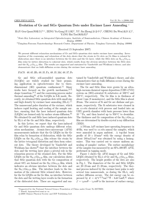
CHIN.PHYS.LETT.Vol.25,No.1(2008)242 Evolution of Ge and SiGe Quantum Dots under Excimer Laser Annealing∗HAN Gen-Quan(韩根全)1∗∗,ZENG Yu-Gang(曾玉刚)1,YU Jin-Zhong(余金中)1,CHENG Bu-Wen(成步文)1,YANG Hai-Tao(杨海涛)21State Key Laboratory on Integrated Optoelectronics,Institute of Semiconductors,Chinese Academy of Sciences,Beijing1000832Tsinghua-Foxconn Nanotechnology Research Center,Department of Physics,Tsinghua University,Beijing100084(Received15September2007)We present different relaxation mechanisms of Ge and SiGe quantum dots under excimer laser annealing.Inves-tigation of the coarsening and relaxation of the dots shows that the strain in Ge dots on Gefilms is relaxed by dislocation since there is no interface between the Ge dots and the Ge layer,while the SiGe dots on Si0.77Ge0.23film relax by lattice distortion to coherent dots,which results from the obvious interface between the SiGe dots and the Si0.77Ge0.23film.The results are suggested and sustained by Vanderbilt and Wickham’s theory,and also demonstrate that no bulk diffusion occurs during the excimer laser annealing.PACS:68.65.Hb,68.35.Fx,68.35.Md,68.37.PsGe and SiGe self-assembled quantum dots (SAQDs)are widely studied for their promis-ing application in optoelectronics due to three-dimensional(3D)quantum confinement.[1]Many works have focused on the growth mechanism,[2,3] shape transition,[4,5]and the coarsening process under thermal annealing[6]of the SAQDs in S-K mode.Re-cently,we obtained SiGe quantum dots with small size and high density by excimer laser annealing(ELA).[7] The nanosecond pulse duration of the excimer,which induces rapid heating and cooling of the sample sur-face,ensuring that the laser induced quantum dots (LIQDs)are formed only by surface atoms diffusion.[8] We obtained Ge and SiGe laser induced quantum dots by ELA of the Ge and SiGefilms,respectively.In this Letter,we report that the laser-induced Ge and SiGe quantum dots undergo different relax-ation mechanisms.Atomic-force-microscopy(AFM) measurements indicate that the Ge LIQDs on the Ge film relax by formation of dislocation,while the SiGe LIQDs on the Si0.77Ge0.23film release the strain by the lattice tetragonal distortion and then form coher-ent dots.The theory developed by Vanderbilt and Wickham has shown[9]that the interface between the dots and the wetting layer plays a pivotal role in the relaxation process of the strained dots.For the SiGe LIQDs on the Si0.77Ge0.23film,our calculation shows that SiGe quantum dots with the Ge composition of about83%are formed on the Si0.77Ge0.23film,which indicates an obvious interface between the dots and the Si0.77Ge0.23film.The interface leads to the for-mation of the coherent SiGe relaxed dots.However, for the Ge LIQDs on the Gefilm,no interface between the dots and the wetting layer results in the formation of the dislocated dots.These are suggested and sus-tained by Vanderbilt and Wickham’s theory,and also demonstrates that no bulk diffusion occurs during the excimer laser annealing.The Ge and SiGefilms were grown by an ultra-high-vacuum chemical vapour deposition(UHV-CVD) system on(001)-oriented Si substrates at500◦C and 550◦C,respectively.The Gefilm is in thickness of about1nm(8monolayers),and the SiGefilm is about 20nm.The sources of Si and Ge are disilane and ger-mane,respectively.The Si substrates were cleaned in an ex-situ chemical etch process and loaded into an UHV growth chamber with basic pressure lower than 10−7Pa,and then heated up to950◦C to deoxidize. The thickness and Ge composition of the Si0.77Ge0.23film are determined by double-crystal x-ray diffraction (XRD).A193nm ArF excimer laser operating frequency in 40Hz,was used to ex-situ anneal the samples,which were annealed in argon ambient.A top-flat beam profile of10×10mm2with the energy density of about180mJ/cm2was obtained by using a homog-enizer.This was carried out to ensure uniform an-nealing of samples’surface.The surface morphology of the samples was measured by an SPA-300HV AFM, performed in tapping mode.Figure1shows the AFM images of Ge and SiGe LIQDs obtained by ELA of Ge and Si0.77Ge0.23films, respectively.The height profiles of the dots are also in Fig.1.The diameters of the Ge and SiGe LIQDs are20–25nm and15–20nm,respectively.The ther-mal process induced by the excimer laser pulse is only several tens nanoseconds,so during the ELA,only surface diffusion occurs.The dot energy can be ex-pressed by E=4ΓV2/3tan1/3θ−6AV tanθ,[2]where Γ=γd cscθ−γs cotθis the increase of surface energy,∗Supported by the National Natural Science Foundation of China under Grant No60576001.∗∗Email:hgquan@c 2008Chinese Physical Society and IOP Publishing LtdNo.1HANGen-Quan et al.243γs and γd are the surface energy per unit area of the wetting layer and dot facet,respectively,θis the facet angle with respect to the surface of the wetting layer,V is the volume of the dot,A =σ2(1−ν)/(2πG )where σis the in-plane misfit strain,and νand G are Poisson’s ratio and shear modulus,respectively.For the LIQDs,only surface energy should be stud-ied,and the second term on the right can be con-sidered as the effect of strain on the surface energy.From the formula,we can see that the slightly strained dots are not stable during the ELA.We speculate that the heavily strained LIQDs will grow,relax the strainin them with longer annealing time.To investigate the relaxation of the LIQDs,we prolong the anneal-ing time with the laser energy density of 180mJ/cm 2.As the ELA continues,We observe the relaxation and the shrinking of the LIQDs,while it is surprisingly found that Ge quantum dots on the Ge wetting layer and SiGe dots on the Si 0.77Ge 0.23layer underwent the different relaxation modes:the Ge dots relax through the formation of the dislocation,while the strain in the SiGe quantum dots on the Si 0.77Ge 0.23wetting layer is released by lattice tetragonal distortion.Fig.1.AFM images (500nm ×500nm)of LIQDs:(a)Ge LIQDs on the Ge film and the height profiles along the line marked,(b)SiGe LIQDs on the Si 0.77Ge 0.23film and the height profiles along the line marked.Figure 2shows a series of AFM images of the mor-phology of Ge LIQDs on the Ge film at different an-nealing times.When the annealing time is prolonged to 3.5hours,coarsening of the quantum dot,as shown in Fig.2(a),occurs.The contacting of the small and large dots in Fig.2(a)and 2(b)can be interpreted to be the losing materials of small dots to the near large dots,which is analogous to the anomalous coarsening in the SAQDs.[10]As the ELA proceeds,the density of the dots further decreases,and when the annealing time is up to 5hours,almost all the LIQDs disappear (shown in Fig.2(c)).After 7-h ELA,no new LIQDs are observed.We speculate that the relaxation of the laser induced Ge dots is by the dislocations and the strained film is also relaxed by the dislocations.Fig-ure 3shows the schematic of the relaxation process ofthe Ge quantum dots on the Ge film.Figure 4(a)shows the coarsening and the growth of the SiGe dots on the Si 0.77Ge 0.23film.After 4-h an-nealing,the SiGe dots become larger and the density decreases.As the annealing continues (5h),some new LIQDs appear.This indicates that the growth and disappearing of the SiGe dots give rise to the restora-tion of the strain in the Si 0.77Ge 0.23film.This will decrease the surface energy and increase the strain en-ergy.The recovered stress in the film drives the new LIQDs under ELA.This reveals that the SiGe dots grow and relax to be the coherent dots,i.e.,the strain in the SiGe dots is relaxed by the lattice distortion.Figure 5shows the schematic of the relaxation process of the SiGe quantum dots on the Si 0.77Ge 0.23film.244HAN Gen-Quan et al.Vol.25Fig.2.AFM images (1µm ×1µm)of the Ge LIQDs on the Ge film with different annealing times:(a)annealed for 3.5h,(b)annealed for 4h,(c)annealed for 5h,(d)annealed for 7h.Fig.3.Schematic diagram of the relaxation mode of the Ge quantum dots on the Ge film.Fig.4.AFM images (1µm ×1µm)of the SiGe LIQDs on the Si 0.77Ge 0.23film for different annealing times:(a)annealed for 4h,(b)annealed for 5h.These results reveal the existence of two different relaxation mechanisms:generation dislocation in the dots and formation coherent relaxed dots.When the quantum dots grow,the relaxation of quantum dots is the competing of the lattice distortion (coherent re-laxed dots)with the formation of the dislocation (dis-located relaxed dots).The theory developed by Van-derbilt and Wickham [9]compares the two mechanisms of elastic relaxation and yields a phase diagram of a lattice mismatched system in which all possible mor-phologies are present,i.e.,uniform films,dislocated dots,and coherent dots.No.1HAN Gen-Quan et al.245It was shown by Vanderbilt and Wickham that morphology of the mismatched system is determined by the ratio of the energy of interface between dots and the wetting layer (E interface )to the change of the sur-face energy (∆E surf ).[9]The deposited material wets the substrate firstly,and then the 2D strained film transforms to the 3D quantum dots.If ∆E surf is posi-tive and large,or if the energy of the interface between the dots and the wetting layer is relatively small,the formation of coherently strained dots is not favoured.With an increase in the amount of deposited material,a transition occurs from uniform film to dislocated dots,and the coherently strained dots are not formed.If ∆E surf is positive and small,or if the energy of the dislocated interface is relatively large,with an increase in the amount of deposited material,a transition oc-curs from a uniform film to coherent dots.Further de-position may cause the onset of dislocations.The de-tailed calculation and the phase diagram can be found in Ref.[9].Fig.5.Schematic diagram of the relaxation process of the SiGe quantum dots on the Si 0.77Ge 0.23film.This theory can be used to interpret the differ-ent relaxation modes of the Ge and SiGe dots.It is sure that the pyramidal laser induced Ge dots,with the diameter of about 20–25nm and density of about 6×1010cm −2,do not exhaust the Ge film with the thickness more than 1nm (8monolayers).Because no bulk diffusion occurs during the annealing,atoms intermixing between the dots and the wetting layer need not be considered.We think that the pure Ge LIQDs are formed on the Ge film,i.e.,there is no in-terface between the dots and the wetting layer.For the SiGe LIQDs on the Si 0.77Ge 0.23film,based on the surface chemical potential calculation,we show that the heavily strained SiGe quantum dots must have a misfit above 0.035corresponding to a Ge composi-tion of about 83%,to promise E surf <0(the dots stable under ELA).[7]This indicates the SiGe dots are Ge richer than the Si 0.77Ge 0.23film,which also results from that the surface diffusion coefficient of Ge is 102–103times greater than that of Si.[11]If the atoms interdiffusion is neglected,there should be an obvious interface between the SiGe quantum dots and the Si 0.77Ge 0.23wetting layer.It is suggested theoret-ically by Vanderbilt and Wickham and supported by our experiments that the interface between the quan-tum dots and the wetting layer plays a pivotal role in the competition between the lattice distortion and the formation of dislocation.Vanderbilt and Wickham’s theory is proven by our results and also confirms and enforces our previous conclusion that the pure Ge dots and an abrupt inter-face between the dots and wetting layer are availablewhich is attributed to no bulk atoms diffusion under ELA.In conclusion,we have studied the different relax-ation mechanisms of the Ge and SiGe quantum dots on Ge and Si 0.77Ge 0.23films,respectively,under ELA.We recover the pivotal role of the interface between the dots and the wetting layer.The relaxation of Ge dots by dislocation is attributed to no interface between Ge dots and the Ge layer,and that of SiGe dots by lattice tetragonal distortion results from the obvious interface between SiGe dots and the Si 0.77Ge 0.23film.This is sustained by Vanderbilt and Wickham’s theory.References[1]Baribeau J M,Wu X,Rowell N L and Lockwood D J 2006J.Phys.:Condens.Matter 18R139[2]TersoffJ and LeGoues F K 1994Phys.Rev.Lett.723570[3]Sutter P,Schick I,Ernst W and Sutter E 2003Phys.Rev.Lett.91176102[4]Rastelli A,Stoffel M,TersoffJ,Kar G S and Schimidt O G2005Phys.Rev.Lett.95026103[5]Montalenti F,Raiteri P,Migas D B,von K¨a nel H,RastelliA,Manzano C,Costantini G,Denker U,Schimidt O G,Kern K and Miglio L 2004Phys.Rev.Lett.93216102[6]Kamins T I,Medeiros-Ribeiro G,Ohlberg D A A andWilliams R S 1999J.Appl.Phys.851159[7]Han G Q,Zeng Y G,Yu J Z,Cheng B W and Yang H T2007J.Cryst.Growth (submitted)[8]Misra N,Xu L,Pan Y L,Cheung N and Grigoropoulos CP 2007Appl.Phys.Lett.90111111[9]Vanderbilt D and Wickham L K 1991Mater.Res.Soc.Symp.Proc.202555[10]Rastelli A,Stoffel M,TersoffJ,Kar G S and Schmidt O G2005Phys.Rev.Lett.95026103[11]Huang L,Liu F,Lu G-H and Gong X G 2000Phys.Rev.Lett.96016103。

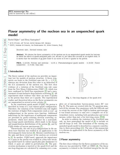
a r X i v :0809.2299v 1 [n u c l -t h ] 12 S e p 2008EPJ manuscript No.(will be inserted by the editor)Flavor asymmetry of the nucleon sea in an unquenched quark modelRoelof Bijker 1and Elena Santopinto 21ICN-UNAM,AP 70-543,04510Mexico DF,Mexico2INFN,Sezione di Genova,via Dodecaneso 33,16164Genova,ItalyReceived:date /Revised version:dateAbstract.We discuss the flavor asymmetry of the nucleon sea in an unquenched quark model for baryonsin which the effects of quark-antiquark pairs (u ¯u ,d ¯d and s ¯s )are taken into account in an explicit form.Itis shown that the inclusion of q ¯q pairs leads to an excess of ¯d over ¯u quarks in the proton.PACS.14.20.Dh Protons and neutrons –12.39.-x Phenomenological quark models –11.30.Hv Flavorsymmetries –11.55.Hx Sum rules1IntroductionThe flavor content of the nucleon sea provides an impor-tant test for models of nucleon structure.A flavor sym-metric sea leads to the Gottfried sum rule S G =1/3[1],whereas any deviation from this value is an indication ofthe ¯d/¯u asymmetry of the nucleon sea.The first clear evidence of a violation of the Gottfried sum rule came from the New Muon Collaboration (NMC)[2],which was later confirmed by Drell-Yan experiments [3]and a mea-surement of semi-inclusive deep-inelastic scattering [4].Allexperiments show evidence that there are more ¯dquarks in the proton than there are ¯u quarks.The experimental studies and theoretical ideas on the flavor asymmetric sea are summarized in several review articles [5].In the constituent quark model (CQM),the proton is described in terms of a uud valence-quark configuration.Therefore,the violation of the Gottfried sum rule implies the existence of higher Fock components (such as uud −q ¯q configurations)in the proton wave function.Additional indications for the importance of multiquark components are provided by parity-violating electron scattering ex-periments,which have shown evidence for a nonvanish-ing strange quark contribution,albeit small,to the charge and magnetization distributions of the proton [6],and by CQM studies of baryon spectroscopy [7].Theoretically,the role of q 4¯q configurations in the nu-cleon wave function was studied in an application to the electromagnetic form factors [8].Mesonic contributions to the spin and flavor structure of the nucleon are reviewed in [5].In another,CQM based,approach the importance of s ¯s pairs in the proton was studied in a flux-tube break-ing model based on valence-quark plus glue dominance to which s ¯s pairs are added in perturbation [9].The pair-creation mechanism is inserted at the quark level and the one-loop diagrams are calculated by summing over a com-Fig.1.One-loop diagram at the quark levelplete set of intermediate baryon-meson states BC (see Fig.1).The pairs are created with the 3P 0quantum num-bers of the vacuum.For consistency with the OZI-rule and to retain the success of the CQM in hadron spectroscopy,it was found necessary to sum over a complete set of in-termediate states,including both pseudoscalar and vector mesons,rather than just a few low-lying states [9,10].In order to address the violation of the Gottfried sum rule,we have generalized the model of [9]to include u ¯u and d ¯d loops as well.The formalism of the ensuing un-quenched quark model is described in a separate contribu-tion to these proceedings [11].The aim of this manuscript is to discuss an application to the flavor asymmetry of the nucleon sea.2Flavor asymmetryThe first clear evidence for the flavor asymmetry of the nu-cleon sea was provided by NMC at CERN [2].The flavor asymmetry is related to the Gottfried integral for the dif-2Roelof Bijker,Elena Santopinto:Flavor asymmetry of the nucleon sea in an unquenched quark model Table1.Experimental values of the Gottfried integralNMC40.004<x<0.800.2281±0.0065HERMES2.30.020<x<0.300.23±0.02E866/NuSea540.015<x<0.350.255±0.008x=131dx ¯d(x)−¯u(x) .Under the assumption of aflavor symmetric sea¯d(x)=¯u(x)one obtains the Gottfried sum rule S G=1/3.The final NMC value is0.2281±0.0065at Q2=4(GeV/c)2 for the Gottfried integral over the range0.004≤x≤0.8 [2],which implies aflavor asymmetric sea.The violation of the Gottfried sum rule has been confirmed by other exper-imental collaborations[3,4].Table1shows that the exper-imental values of the Gottfried integral are consistent with each other within the quoted uncertainties,even though the experiments were performed at very different scales, as reflected in the average Q2values.Theoretically,it was shown that in the framework of the cloudy bag model the coupling of the proton to the pion cloud provides a mecha-nism to produce aflavor asymmetry due to the dominance of nπ+among the virtual configurations[12].In the unquenched quark model,theflavor asymmetry can be calculated from the difference of the number of¯d and¯u sea quarks in the protonN¯d−N¯u= 10dx ¯d(x)−¯u(x) .Even in absence of explicit information on the(anti)quark distribution functions,the integrated value can be ob-tained directly from the left-hand side of Eq.(1).The effect of the quark-antiquark pairs on the Gottfried inte-gral is a reduction of about one third with respect to the Gottfried sum rule,corresponding to an excess of¯d over ¯u quarks in the proton which is in qualitative agreement with the NMC result.It is important to note that in this calculation the parameters were taken from the literature [9,13],and that no attempt was made to optimize their values.Due to isospin symmetry,the neutron has a similar excess of¯u over¯d quarks.3Summary,conclusions and outlookIn this contribution,we discussed the importance of quark-antiquark pairs in baryon spectroscopy.The calculations were carried out in an unquenched quark model for baryons in which the contributions from u¯u,d¯d and s¯s loops are taken into account in a systematic way[11].The model was applied to theflavor asymmetry of the nucleon sea.In afirst,exploratory,calculation in which the parameters were taken from the literature[9,13],it was shown that the inclusion of q¯q pairs leads immedi-ately to an excess of¯d over¯u quarks in the proton.We emphasize again that no attempt was made to optimize the parameters in the calculations.In our opinion thefirst results for theflavor asymme-try(discussed here)and the proton spin(see[11])are very promising and encouraging.We believe that the inclusion of the effects of quark-antiquark pairs in a general and consistent way,as suggested in[11]and in this contribu-tion,may provide a major improvement to the constituent quark model,increasing considerably its range and appli-cability.In future work,the unquenched quark model will be applied systematically to several problems in light baryon spectroscopy,such as the electromagnetic and strong cou-plings,the elastic and transition form factors of baryon resonances,their sea quark content and theirflavor de-composition[14].AcknowledgmentsThis work was supported in part by a grant from CONA-CYT,Mexico and in part by INFN,Italy. References1.K.Gottfried,Phys.Rev.Lett.18,1174(1967).2.P.Amaudruz et al.,Phys.Rev.Lett.66,2712(1991);M.Arneodo et al.,Nucl.Phys.B487,3(1997).3. A.Baldit et al.,Phys.Lett.B332,244(1994);R.S.Towell et al.,Phys.Rev.D64,052002(2001).4.K.Ackerstaffet al.,Phys.Rev.Lett.81,5519(1998).5.S.Kumano,Phys.Rep.303,183(1998);J.Speth and A.W.Thomas,Adv.Nucl.Phys.24,83 (1998);G.T.Garvey and J.-C.Peng,Prog.Part.Nucl.Phys.47,203(2001).6. A.Acha et al.,Phys.Rev.Lett.98,032301(2007).7.See e.g.N∗Physics,Proceedings of the Fourth CE-BAF/INT Workshop,Eds.T.-S.H.Lee and W.Roberts (World Scientific,1997);N.Isgur,Nucl.Phys.A623,37c(1997);R.Bijker,F.Iachello and A.Leviatan,Phys.Rev.D55, 2862(1997);M.Aiello,M.M.Giannini and E.Santopinto,J.Phys.G: Nucl.Part.Phys.24,753(1998);L.Ya.Glozman,W.Plessas,K.Varga and R.F.Wagen-brunn,Phys.Rev.D58,094030(1998);R.Bijker,F.Iachello and A.Leviatan,Ann.Phys.(N.Y.) 284,89(2000);U.L¨o ring,B.Ch.Metsch,H.R.Petry,Eur.Phys.J.A10, 447(2001).8.Q.B.Li and D.O.Riska,Nucl.Phys.A791,406(2007).9.P.Geiger and N.Isgur,Phys.Rev.D55,299(1997).10.P.Geiger and N.Isgur,Phys.Rev.Lett.67,1066(1991);Phys.Rev.D44,799(1991);ibid.47,5050(1993).Roelof Bijker,Elena Santopinto:Flavor asymmetry of the nucleon sea in an unquenched quark model311. E.Santopinto and R.Bijker,these proceedings.12. A.W.Thomas,Phys.Lett.B126,97(1983);E.M.Henley and ler,Phys.Lett.B251,453(1990).13.S.Capstick and W.Roberts,Phys.Rev.D49,4570(1994).14.R.Bijker and E.Santopinto,work in progress.。

这成长历程王振林，男，1965年生，江苏姜堰人。

1996年获南京大学理学博士学位，教授，博士生导师，现任南京大学物理系副主任。

2004年获得国家杰出青年基金，并荣获国家重点基础研究计划(973计划)先进个人称号。

2005年获得教育部提名国家科学技术奖自然科学一等奖（排名第五）。

2006年入选教育部长江计划特聘教授。

求学经历：1983－1987年，苏州大学，物理系，学士学位1987－1990年，苏州大学，物理系，硕士学位（导师李振亚教授）1993－1996年，南京大学，物理系，博士学位（导师闵乃本教授）工作经历：1990－1993年，江南大学，基础课部，讲师1996－1998年，南京大学，物理系，讲师1998－2002年，南京大学，物理系，副教授2003－现在，南京大学，物理学院，教授1999－2000年，香港科技大学，物理系，访问学者2001－2002年，美国加利福尼亚大学伯克利分校，物理系，访问学者从事研究王振林教授的研究方向主要在胶体颗粒自组织现象、光子带隙材料中光传播理论、微纳光子材料制备与控制、微纳光子信息物理与器件在光与微结构材料相互作用，及其异常光学效应机理与应用研究，涉及微纳光子学，微纳光子材料设计、制备，表面等离激元学，近场光学这些研究方面尤为擅长。

主持项目包括国家杰出青年基金资助项目：光在非均匀介质中的传播；国家重大基础研究计划973资助课题：表面等离激元波人工结构材料的能带、制备和新现象研究；国家自然科学基金资助的重点项目：新型金属微纳结构表面等离激元共振激发、传播及其物理效应。

研究价值1996年至今，在Phys. Rev. Lett., Adv. Mater., Adv. Funct. Mater., Appl. Phys. Lett., Phys. Rev. B (A/E), Opt. Lett.等国际重要学术刊物上发表论文80余篇，所发表论文被他引800余次，获得14项国家发明专利授权。

Nanoscience andNanotechnology LettersV ol.5,546–551,2013 Synthesis of Multiferroic Pb(Zr0 52Ti0 48 O3–CoFe2O4 Core–Shell Nanofibers by Coaxial ElectrospinningYing Xie1,Yun Ou1 2,Feiyue Ma2,Qian Yang1,Xiaolan Tan3,and Shuhong Xie1 2 ∗1Faculty of Materials,Optoelectronics and Physics,and Key Laboratory of Low Dimensional Materials andApplication Technology of Ministry of Education,Xiangtan University,Xiangtan,Hunan411105,China2Department of Mechanical Engineering,University of Washington,Seattle,WA98195,U.S.A 3College of Mechanical and Electrical Engineering,North China University of Technology,Beijing,100041,ChinaMultiferroic Pb(Zr0 52Ti0 48 O3–CoFe2O4(PZT–CFO)core–shell nanofibers have been synthesizedby coaxial electrospinning.The core–shell configuration of nanofibers has been verified by scanningelectron microscope and transmission electron microscope,and the spinel structure of CFO andperovskite structure of PZT have been confirmed by X-ray diffraction,high resolution transmissionelectron microscope and selected area electron diffraction.The macroscopic ferromagnetic propertyof core–shell nanofibers has been demonstrated by magnetic hysteresis loop,while the micro-scopic magnetic domain structure of magnetized nanofiber has been revealed by magnetic forcemicroscopy.The surface potential of core–shell nanofiber has been measured by scanning Kelvinprobe microscope,and the piezoelectricity of core–shell nanofiber has been tested by piezore-sponse force microscopy using dual frequency resonance tracking technique,which confirms theferroelectricity of PZT–CFO core–shell nanofibers.Keywords:Multiferroic,Pb(Zr0 52Ti0 48 O3–CoFe2O4,Core–Shell Nanofiber,CoaxialElectrospinning.1.INTRODUCTIONConsiderable developments on nanostructured materials1–3 and their controls4–6created various range of innova-tive functions.Especially,multiferroic composite materials consisting of ferroelectric and ferromagnetic phases have attracted a great deal of attention in the last decade,7–10 wherein the magnetoelectric(ME)effect is induced through the so-call product property,11via mechanical interactions arising from magnetostrictive and piezoelec-tric effects in individual phases.The ME coupling makes it possible to manipulate the electric state of a multiferroic material through a magneticfield,or vice versa,and thus opens door for extensive potential applications,includ-ing multiple-state memory devices that can be electrically written and magnetically read,energy harvester,electri-cally controlled microwave phase shifters or ferromagnetic resonance devices,magnetically controlled electro-optic or piezoelectric devices,and broadband magneticfield sensors.9 12–14In recent years,the investigation of multiferroic materi-als focused on low dimensional hybrid materials including thinfilm,15 16superlattices,17–20and nanocomposites.21–23∗Author to whom correspondence should be addressed.These low dimensional composite materials can providetighter coupling between ferroelectric and ferromagneticphases,and offer additional degrees of freedom in con-trolling the size,interface,and epitaxial strain to enhancethe ME coupling.Indeed,recent theoretical analysis indi-cates that composite multiferroic nanofibers exhibit MEresponses higher than thinfilms of similar compositions,24due to their substantially relaxed substrate constraint,and nanofibers consisting of CoFe2O4(CFO)core andPb(Zr0 52Ti0 48 O3(PZT)shell with enhanced ME coupling has been successfully demonstrated.25This motivates us todevelop multiferroic nanofibers consisting of PZT core andCFO shell instead.Among various techniques for synthesis of one-dimensional core–shell nanostructures,such as wetetching26 27and anodized aluminum oxide(AAO)template-electrodeposition,28 29electrospinning30 31is es-pecially convenient and versatile,and has been adopted tosynthesize polymeric,32ceramic,33and metallic nanofiberswith various morphologies,including both core–shell andhollow types.34 35Here we demonstrate the synthesis ofPZT–CFO core–shell multiferroic nanofibers by coaxialelectrospinning,and examine their morphology,crystallinestructure,as well as the multiferroic properties.2.EXPERIMENTAL DETAILS2.1.Material SynthesisMultiferroic PZT–CFO core–shell nanofibers have been synthesized by sol–gel process and coaxial electrospin-ning.The preparations of PZT and CFO precursors with concentration of 0.2mol/L were described in our early work.36Poly(vinyl pyrrolidone)(PVP)with molecular weight of 1,300,000was added to PZT and CFO pre-cursors respectively,and stirred continuously to form homogeneous solutions,with the concentration of PVP controlled around 0.035g/mL.These two solutions were then electrospun using a coaxial spinneret as schemati-cally shown in Figure 1.It consists of two commercial blunt needles with different diameters and lengths assem-bled into a coaxial structure.During the electrospinning process,the syringe loaded with PZT precursor was con-nected vertically to the needle with 0.7mm outside diam-eter as solution for core,and the syringe loaded with CFO precursor was connected horizontally to the needle with 1.28mm outside diameter as solution for shell.The core solution was driven by a syringe pump (NE-500,New Era Pump Systems,Inc.)at a rate of 0.3mL/h,while the shell solution was driven at a rate of 0.48mL/h.The needle was connected to a high-voltage power supply (ES40P-5W,Gamma High V oltage,Inc.),and the distance between the needle tip and substrate was about 16cm,with the elec-tric field strength approximately 1.2kV/cm,which pro-vide enough repulsive electrostatic force to overcome the surface tension of the electrospinning solution and eject nanofiber from the tip of the Taylor cone.The electrospun nanofibers were collected to Pt/Ti/SiO 2/Si substrates,dried at 120 C for 4h,followed by heating at 400 C and then thermal annealing at 750 C for 2h in air.2.2.Material CharacterizationThe morphology of nanofibers was examined by scanning electron microscopy (SEM,FEI Sirion)andtransmissionFig.1.The schematic set up of coaxial electrospinning system.electron microscopy (TEM,FEI Tecnai).The crystalline structure of nanofibers was examined by selected area electron diffraction (SAED,FEI Tecnai)as well as X-ray diffraction (XRD,Bruker D8Focus)with Cu K radiation ( =0 15406nm).The macroscopic ferromagnetic prop-erty of nanofibers was measured by Lakeshore vibrating sample magnetometer (VSM).To increase the magnetic response of the core shell nanofibers,the specimen (nano-fibers with Pt/Ti/SiO 2/Si substrate)was magnetized under a large in-plane magnetic field of 7000Oe for 20minutes by using an electromagnet (GMW Electromagnet Model 3473).The magnetic domain structure of nanofibers was examined by magnetic force microscopy (MFM)using an Asylum Research MFP-3D atomic force microscope (AFM),and a 45nm CoPt/FePt alloy coated silicon tip with a coercivity higher than 5000Oe was used as the probe,which was magnetized along the tip axis using an NdFeB permanent magnet.The tapping mode set point was fixed at 0.4V with approximately 40nm distance between the tip and sample during the initial topography scan,and delta height and driving amplitude were set at 50nm and 20mV during the subsequent scan for magnetic image.To characterize the surface potential of nanofibers,scanning Kelvin probe microscopy (SKPM)was used with tip voltage set to be 3.0V .The ferroelectricity of nano-fibers was measured by piezoresponse force microscopy (PFM)using an Asylum Research MFP-3D,as described in our earlier paper.373.RESULTS AND DISCUSSIONThe morphology of PZT–CFO core–shell nanofibers was examined by SEM,as shown in Figure 2.The typical sur-face SEM image of the nanofibers is given in Figure 2(a),and it is observed that the diameter of nanofibers is in the range of 100to 200nm.The cross-section topogra-phy of the nanofibers is shown in Figure 2(b),where the core–shell structure is evident,though some gaps exist at interfaces between the PZT core and CFO shell due to the different shrinkage of ceramic fibers during calcination.Such interface structure is not desirable for ME coupling,and we are currently working on increasing interface bond-ing by fine tuning the processing parameters.The core–shell structure of the nanofiber is further confirmed by TEM image,as seen in Figure 3(a),where it is observed that the nanofiber is composed of dense PZT grains and porous CFO grains.The interface between PZT core and CFO shell,though perturbed,is clearly visible.From the TEM image,it is estimated that the outer diameter of CFO shell is approximately 150nm,whereas the diameter of the PZT core is approximately 60nm.This is consistent with different flow rates for PZT and CFO during electro-spinning.The perovskite structure of PZT and spinel structure of CFO are confirmed by SAED pattern in Figure 3(b)show-ing that both CFO and PZT phases exist in the nanofiber,Fig.2.SEM images of PZT–CFO core shell nanofibers:(a)surface topography and (b)cross sectiontopography.Fig.3.TEM and SAED images of PZT–CFO core–shell nanofiber:(a)TEM image,(b)SAED pattern and (c)HRTEMimage.Fig.4.XRD pattern of PZT–CFO core shellnanofibers.Fig.5.VSM magnetic hysteresis loops of PZT–CFO and CFO-PZT core shell nanofibers.and it is observed the amount of CFO shell is much more than that of PZT core,consistent with the diameter distri-bution observed in Figure 3(a).The polycrystalline nature of core–shell nanofiber is also clear from the SAED ringFig.6.MFM images of PZT–CFO core shell fiber:(a)topography and (b)phase.(Scan size 0.375um ×1.5um).pattern.The crystalline structure of PZT and CFO phases are also confirmed by HRTEM as shown in the Figure 3(c),where two lattice spaces are measured to be 0.285nm and 0.253nm,corresponding (110)plane of PZT phase and (311)plane of CFO phase,respectively.The inter-face between PZT shell and CFO core is not very sharp owing to the intermiscibility of PZT and CFO electrospin-ning solution,which is consistent with previous report for PZT–CFO composite materials.38The crystalline phases of core–shell nanofibers are further examined by XRD,as shown in Figure 4,where two distinct sets ofdiffractionFig.7.Surface potential distribution of PZT–CFO core shell nanofiber:(a)topography,(b)surface potential and (c)position dependence of the surface potential along the solid line in (b).peaks are observed,corresponding to perovskite PZT and spinel CFO phases,respectively.It is also observed that the amount of CFO shell is higher than that of PZT core,consistent with the TEM result.Room temperature ferromagnetism of core–shell nano-fibers is confirmed by magnetic hysteresis loop using VSM,as shown in Figure 5.The remnant magnetization for the PZT–CFO core–shell nanofibers is measured to be 7.50emu/g,larger than 3.4emu/g that was measured from CFO-PZT core shell nanofibers.25The corresponding coercive field is measured to be 700Oe,similar to CFO-PZT core shell nanofibers,while higher than 576Oe that was measured from random hybrid PZT–CFO nanofibers.36These results are reasonable as the concentration of CFO in the PZT–CFO nanofibers is higher than that in the CFO-PZT nanofibers,as confirmed in Figures 2and 3,resulting in larger magnetization.In the core–shell nanofibers,the CFO layer is constrained by PZT layer,making it harder for magnetic domains to switch and resulting in higher coercive field,as we observed here.39The AFM topography and corresponding MFM phase images of the PZT–CFO nanofiber are shown in Figure 6.Both images show a heterogeneous microstructure.The diameter of nanofiber is around 150nm with height less than 100nm,as revealed by the topographic image in Figure 6(a).The magnetic domain pattern of magnetized PZT–CFO nanofiber is shown in Figure 6(b),and irregu-lar domains are observed,with yellow areas corresponding to a stronger magnetic field and blue areas indicating aDelivered by Publishing Technology to: Peter Derycz IP: 216.185.156.28 On: Tue, 25 Jun 2013 18:07:29Copyright American Scientific Publishersweak magnetic field.40Furthermore,the AFM topographic and corresponding surface potential distribution of another PZT–CFO nanofiber is shown in Figure 7.The topogra-phy in Figure 7(a)is similar to Figure 6(a),though the diameter is larger than that of Figure 6(a),about 200nm.The mapping of surface potential is shown in Figure 7(b),and a corresponding line scan is given in 7(c).The surface potential contrast between the core–shell nanofiber and the conductive substrate is evident from Figure 7(b),due to the spontaneous polarization of the nanofiber that attracts free charges.It is interesting to observe that the fringe region of nanofiber has higher surface potential while the central region of nanofiber has lower potential,and the poten-tial difference is approximately 0.2V .This is believed to be caused by the accumulation of charges at nanofiber-substrate interface,and thus confirms the piezoelectricity of the core–shell nanofibers.The ferroelectricity of the core–shell nanofibers is fur-ther confirmed by vertical PFM with dual frequency res-onance tracking (DFRT)technique,which reduces the crosstalk due to the shift in resonance frequency by track-ing the contact resonance frequency using a feedback loop Fig.8.Piezoelectric force microscopy (PFM)images of PZT–CFO core shell nanofiber:(a)topography,(b)intrinsic amplitude and (c)phase at resonant frequency,and (d)quality factor.and allows determination of resonance frequency 0,qual-ity factor Q ,amplitude A 0and phase 0at resonance frequency simultaneously.41 42It is used for quantitative analysis,with the intrinsic vertical piezoresponse of the core–shell fiber determined by correcting the quality fac-tor Q ,37as shown in Figure 8.The topography image in Figure 8(a)reveals that two nanofibers are bond together with diameter around 400nm,and the height roughness is also less than 100nm.It is observed in Figure 8(b)that the max intrinsic amplitude in the central region of fiber is around 16pm due to the presence of PZT core,while the amplitude at the fringe region is close to 0pm owing to CFO shell.It is also obvious that the substrate has no piezoresponse.Phase contrast mapping in Figure 8(c)further exhibits the difference of polar distribution in the probed fibers,and the width of phase image is narrower than that of topography image,which confirms the ferro-electricity and core–shell structure of the nanofibers.The corresponding mapping of quality factor Q (Fig.8(d))indi-cates that the variation of quality factor Q on the fibers is large ranging from 10to 60,and this reflects difference in energy dissipation at different locations of nanofibers.374.CONCLUSIONIn summary,polycrystalline PZT–CFO core–shell nano-fibers have been synthesized by coaxial electrospin-ning in combination with sol–gel process,and their microstructures have been thoroughly examined.Multifer-roic properties of PZT–CFO core–shell nanofibers have also been verified by macroscopic magnetic hysteresis loop,microscopic MFM mapping,surface potential map-ping of SKPM and dual frequency piezoresponse force microscopy.The nanofibers thus canfind a variety of applications as a one-dimensional multiferroic materials. Acknowledgments:We acknowledge the support of US National Science Foundation(DMR-1006194and CMMI1100339),Natural Science Foundation of China (Approval Nos.10902095,10972189and11102175),Bei-jing Natural Science Foundation(3122014)and Educa-tional Commission of Hunan Province(YB2011B028), China.References and Notes1.K.Ariga,A.Vinu,Y.Yamauchi,Q.Ji,and J.P.Hill,Bull.Chem.Soc.Jpn.85,1(2012).2.X.Pan,Y.Zhao,and Z.Fan,Nanosci.Nanotechnol.Lett.4,463(2012).3.K.M.Kummer,E.Taylor,and T.J.Webster,Nanosci.Nanotechnol.Lett.4,483(2012).4.K.Ariga,T.Mori,and J.P.Hill,Adv.Mater.24,157(2012).5.L.Sun,S.Zhang,Q.Wang,and D.Zhao,Nanosci.Nanotechnol.Lett.4,471(2012).6.Q.Zhang,H.Xu,and W.Yan,Nanosci.Nanotechnol.Lett.4,505(2012).7. C.W.Nan,M.I.Bichurin,S.X.Dong, D.Viehland,andG.Srinivasan,J.Appl.Phys.103,031101(2008).8.J.Y.Zhai,Z.P.Xing,S.X.Dong,J.F.Li,and D.Viehland,J.Am.Ceram.Soc.91,351(2008).9.J.F.Scott,Nat.Mater.6,256(2007).10.N.A.Spaldin and M.Fiebig,Science309,391(2005).11. C.W.Nan,Phys.Rev.B50,6082(1994).12.Y.K.Fetisov and G.Srinivasan,Appl.Phys.Lett.88,143503(2006).13.R.Ramesh and N.A.Spaldin,Nat.Mater.6,21(2007).14.J.Ma,J.Hu,Z.Li,and C.W.Nan,Adv.Mater.23,1062(2011).15.J.G.Wan,X.W.Wang,Y.J.Wu,M.Zeng,Y.Wang,H.Jiang,W.Q.Zhou,G.H.Wang,and J.M.Liu,Appl.Phys.Lett.86,122501 (2005).16. C.Deng,Y.Zhang,J.Ma,Y.Lin,and C.W.Nan,J.Appl.Phys.102,074114(2007).17. E.Bousquet,M.Dawber,N.Stucki,C.Lichtensteiger,P.Hermet,S.Gariglio,J.M.Triscone,and P.Ghosez,Nature452,732(2008).18.M.P.Singh,W.Prellier,C.Simon,and B.Raveau,Appl.Phys.Lett.87,022505(2005).19.J.Zhang,J.Dai,W.Lu,and H.Chan,J.Mater.Sci.44,5143(2009).20.P.Murugavel,M.P.Singh,W.Prellier,B.Mercey,C.Simon,andB.Raveau,J.Appl.Phys.97,103914(2005).21.H.Zheng,J.Wang,S.E.Lofland,Z.Ma,L.Mohaddes-Ardabili,T.Zhao,L.Salamanca-Riba,S.R.Shinde,S.B.Ogale,F.Bai,D.Viehland,Y.Jia,D.G.Schlom,M.Wuttig,A.Roytburd,andR.Ramesh,Science303,661(2004).22.J.Cheng,S.Yu,J.Chen,Z.Meng,and L.E.Cross,Appl.Phys.Lett.89,122911(2006).23.W.M.Zhu,H.Y.Guo,and Z.G.Ye,Phys.Rev.B78,014401(2008).24. C.L.Zhang,W.Q.Chen,S.H.Xie,J.S.Yang,and J.Y.Li,Appl.Phys.Lett.94,102907(2009).25.S.H.Xie,F.Y.Ma,Y.M.Liu,and J.Y.Li,Nanoscale3,3152(2011).26.J.M.Romo-Herrera,R.A.Alvarez-Puebla,and L.M.Liz-Marzan,Nanoscale3,1304(2011).27.J.Hwang,B.Min,J.S.Lee,K.Keem,K.Cho,M.Y.Sung,M.S.Lee,and S.Kim,Adv.Mater.16,422(2004).28. C.Y.Tung,G.Detlef,M.Stephan,Y.M.Y.Eric,A.Sebastian,B.Julien,and N.Kornelius,Adv.Mater.22,2435(2010).29.S.Panigrahi and D.Basak,Nanoscale3,2336(2011).30. F.Yao,L.Q.Xu,B.P.Lin,and G.D.Fu,Nanoscale2,1348(2010).31.J.T.McCann,D.Li,and Y.Xia,J.Mater.Chem.15,735(2005).32.Z.M.Huang,Y.Z.Zhang,M.Kotaki,and S.Ramakrishna,Compos.Sci.Technol.63,2223(2003).33.M.H.Tang,W.Shu,F.Yang,J.Zhang,G.J.Dong,and J.W.Hou,Nanotechnology20,385602(2009).34.S.Zhan,D.Chen,X.Jiao,and C.Tao,J.Phys.Chem.B110,11199(2006).35. B.G.Lu,X.S.Guo,Z.Bao,X.D.Li,Y.X.Liu,C.Q.Zhu,Y.Q.Wang,and E.Q.Xie,Nanoscale3,2145(2011).36.S.H.Xie,J.Y.Li,Y.Qiao,Y.Y.Liu,n,Y.C.Zhou,andS.T.Tan,Appl.Phys.Lett.92,062901(2008).37.S.H.Xie,A.Gannepalli,Q.N.Chen,Y.M.Liu,Y.C.Zhou,R.Proksch,and J.Y.Li,Nanoscale4,408(2012).38.L.Rueijer,W.Tai-Bor,and C.Ying-Hao,Scripta Mater.59,897(2008).39.R.C.O’Handley,Modern Magnetic Materials:Principles and Appli-cations,Wiley,New York(1999).40.M.Hehn,S.Padovani,K.Ounadjela,and J.P.Bucher,Phys.Rev.B54,3428(1996).41.T.R.Albrecht,P.Grutter,D.Horne,and D.Rugar,J.Appl.Phys.69,668(1991).42. B.J.Rodriguez, C.Callahan,S.V.Kalinin,and R.Proksch,Nanotechnology18,475504(2007).Received:31August2012.Accepted:29December2012.。

Optically Controllable Photonic Structures with Zero AbsorptionChris O’Brien*and Olga KocharovskayaDepartment of Physics and Astronomy and Institute for Quantum Studies,Texas A&M University,College Station,Texas77843-4242,USA(Received27May2011;revised manuscript received11August2011;published21September2011) We show the possibility to periodically modulate the refractive index in a homogeneous resonant atomic medium in space or/and time while simultaneously keeping vanishing absorption or gain.Such modulation is based on periodic resonant enhancement of the refractive index,controlled by an external opticalfield,and opens the way to produce coherently controllable photonic structures.We suggest the possible implementation of the proposed scheme in rare-earth doped crystals with excited state absorption.DOI:10.1103/PhysRevLett.107.137401PACS numbers:78.20.Ci,42.50.Gy,42.65.AnOne,two,or three-dimensional periodic heterostructures made of two dielectric materials with different refractive indices,such as distributed Bragg reflectors(DBRs),holey fibers,or photonic crystalsfind many applications,includ-ing reflective coatings,distributed feedback lasers,and optical cavities.Different technologies such as photoli-thography,etching,drilling,and self-assembling are used for construction of such structures.We suggest a method to produce transparent photonic structures in a homogeneous resonant atomic media,such as dielectrics with homogeneously distributed impurities, atomic,or molecular gases,simply by illuminating these materials with standing waves of a laserfield.Such opti-cally produced photonic structures could easily be con-trolled(including switching on or off,changing amplitude and period of modulation)and would be highly selective in frequency,naturally limited by the width of the optical resonance.Refractive index(RI)is strongly enhanced near atomic resonances.However,that enhancement is accompanied by enhancement of ly,when the maximal contribution from the atomic resonance to the RI is reached,the contribution to the absorption is on the same order which prevents the usage of obtained RI.There have been several proposals on how to resonantly enhance the refractive index while at the same time eliminating reso-nant absorption.One approach is based on interference effects in multilevel atomic systems driven by coherent resonantfields[1–5].Another suggestion is to compensate absorption with resonant gain from an inverted transition [6].Such a situation could be realized either in a mixture of two two-level atomic species,or in a single atomic species possessing simultaneously both noninverted and inverted transitions with slightly shifted frequencies[7].Proof of principle experiments were done in hot Rb vapors in which enhancement of the refractive indexÁn$10À4was achieved under negligible absorption[8,9].An enhance-ment up to the valueÁn$10À2is expected with an increase of density to N¼6Â1016cmÀ3.The further increase of the refractive index in room-temperature gases is not feasible due collisional broadening becoming the dominant contribution to the linewidth.Much higher reso-nant additions to the background index are anticipated in transition element doped crystals due to the essentially higher density of the ions which does not in general result in proportional line broadening[7,10,11].In all of these proposals the RI was uniform in space. Moreover,an enhancement of the RI with vanishing reso-nant absorption was achieved only at a particular detuning of the probefield from atomic resonance and was accom-panied by either absorption or gain at the neighboring detunings.Thus,none of those proposals were suitable for achieving spatial modulation of the refractive index with zero absorption.Our proposal is based on spatial modulation of the energy of a populated intermediate state in a nearly degenerate ladder configuration via the ac-Stark effect in a standing wavefield which results in a spatially dependent detuning leading to a periodic resonant increase and decrease of the refractive index in space while simul-taneously keeping transparency of the medium. Consider the interaction of a probefield with a medium of three level atoms in a ladder configuration such that the probefield interacts with both transitions as illustrated in the inset of Fig.1.The transition frequencies!21and!32 are close to each other so that the probefield with fre-quency!p interacts simultaneously with both transitions and for a weak probe Rabi frequency p( 21, 32the susceptibility is defined as the sum of the susceptibilities of two two-level transitions:¼3N38rad21ð 1À 2Þ21Ài 21þrad32ð 2À 3Þ32Ài 32:(1)Here N is the atomic density,the detunings are defined as 21¼!21À!p and 32¼!32À!p, is the probefield wavelength in the medium, rad ij is the radiative decay rate for the i to j transition, ij is the total decoherence rate,and i is the population in the i th energy level.We assume thatthe amplitudes of both transitions are matched but of opposite sign:rad 21ð 1À 2Þ¼À rad32ð 2À 3Þ;(2)which means that one of the two transitions is inverted.Letit be transition 2-1,i.e. 2À 1>0.We also assume the widths of the transitions are equal 21¼ 32and the probe field is tuned to two-photon resonance,i.e.!p ¼!31=2.Thus for arbitrary position of level 2the blue detuning of the probe field from one of two two-level transitions is equal to the red detuning from the other,i.e., 32¼À 21¼ ,leading to the remarkable property that gain at one transition and absorption at another one cancel each other while the real part of susceptibility is doubled.So,the susceptibility is purely real:¼3N 3 rad 21ð 1À 2Þ8 22 2þ 221:(3)It means that the probe field neither experiences absorptionnor gain independently of level 2’s energy,i.e.,for arbitrary values of .At the same time the resonant susceptibility varies from the minimum to the maximum value as is shifted from À to as shown in Fig.1.If the energy of the intermediate level is modulated in space along the direction of propagation of the probe field,the refractive index is also modulated.Such spatial modulation can be produced along the optical axis via the ac-Stark shift.A control laser field E s cos ð!s t Þapplied at the 0-2transition adjacent to the 1-2transition and far detuned from this transition Ás ¼!s À!20) 20would result in a split-ting of the intermediate state 2into two ac-Stark sublevels shifted in frequency by Àj s j 2=Ás and Ás þj s j 2=Ás ,respectively,where s is the associated Rabi frequency.The probe field is far out of resonance with the transitions from the second Stark sublevel from both level 1and level 3and,therefore its interaction with these transitions is neg-ligible while the first Stark sublevel is slightly shifted fromthe original level 2and strongly interacts with the probefield.In other words,the susceptibility at each transition (2-1or 2-3),which in general consists of two terms asso-ciated with the one-photon and two-photon resonances is reduced to the one-photon contribution and has the same form as given by Eq.(3),just with shifted transition frequencies.If the control field represents itself as a standing wave such that the Rabi frequency is a function of position inside the medium, s ðz Þ¼ s cos ðk s z Þ,then the ac-Stark shift of level 2is given by:ÁE ¼À@j s j 2s À@j s j 2scos ð2k s z Þ:(4)Thus it consists of a constant shift,j s j 2=2Ás ,and a sinu-soidal modulation,ðj s j 2=2Ás Þcos ð2k s z Þ.If the difference between the atomic transition frequencies !32À!21is chosen to be equal to Àj s j 2=Ás then the susceptibility is described by Eq.(3)with ¼ðj s j 2=2Ás Þcos ð4 z= s Þ(where s is the wavelength of the control field in the medium).Hence the refractive index will be modulated symmetrically with respect to its background value as shown in Fig.2.The spacial period s =2is defined by the wavelength,while the modulation depth Àj s j 2=Ás is defined by the Rabi frequency of the modulating field s .To provide the maximum amplitude of refractive index modulation the Rabi frequency of the control field should meet the condition 2s ¼2 Ás .With a strong enough index variation a transparent for a particular frequency 1-D photonic crystal can be created with properties that are optically controlled.Similarly a 2D or 3D photonic structure can be produced by application of 2or 3orthogonal modulating control fields.Even for index variations much smaller than the background RI the me-dium will behave as a distributed Bragg reflector if s ’ p specifically,when the wavelength mismatch is within the width of the Bragg band gap, s À p < s Án=ð n bg Þ.Since the medium remains transparent,many periods of spatial RI structures can be used as needed to achieve the required reflection coefficient.When the probe field is detuned from two-photon reso-nance with 1-3transition it will experience either gain or0.51.01.52.0zs1.00.50.51.0ReMaxFIG.2(color online).Real part of the susceptibility plotted as a function of position along the opticalaxis.21Re MaxFIG.1(color online).Real part of the susceptibility as a function of the level shift .Note that the imaginary part is identically zero.Inset:the energy level diagram for the corre-sponding three-level scheme.absorption.The question arises if such gain may result in the building up of a spontaneously amplified field empty-ing the inverted transition and limiting the propagation length of the probe field in the medium with periodic refractive index.Fortunately,this is not the case.Indeed,since the position of the intermediate level is periodically modulated in space,then a detuned probe field experiences periodically interchanging regions of gain and absorption suppressing the development of such an instability as can be seen in Fig.3.In fact averaging the absorption over a wavelength s shows that the medium is effectively trans-parent even when the probe field is detuned from resonance.The simple model of a ladder system previously dis-cussed assumed the existence of two transitions possessing equal linewidths,equal products of transition strength and population difference,and nearly degenerate (on the scale of the linewidth)frequencies.It is difficult if not impos-sible to meet these conditions in a real atomic system.However,it is possible to construct an effective ladder system whose upper transition has controllable parameters which could be optically tuned to satisfy these conditions.It can be accomplished by adding to the original simple ladder system along with the modulating control field E s coupled to an adjacent transition 0-2(as discussed above)a second control field E c coupling the excited state 3to an additional unpopulated level 4as shown in Fig.4.This second far-detuned control field (Ác ) rad 32, c where Ác ¼!43À!c and c is the control field Rabi fre-quency)is chosen to satisfy approximately the two-photon resonance condition:!c À!p ¼!42,forming together with the probe field a far-detuned lambda scheme.A strong far-detuned field results in an ac-Stark splitting of level 3and the response to the probe field consists of two terms representing one-photon (upper Stark sublevel)and two-photon (lower Stark sublevel)contributions in the same way as previously discussed.But now it is the two-photon contribution which plays a dominant role due to the two-photon resonance condition [7,12].As a result,the total five level system under the formu-lated above conditions is reduced to an effective three-level ladder system with the lower transition 1-2’’and the upper transition 2’’-3’.Its susceptibility takes the form:res¼3N 38 2rad 21p=ð2Àp Þ p þ 2s 2Ás þ Ài 21þ rad32=½ð2Àp Þð1þ2 Þ p À!32þ!21À 2s 2ÁsÀ þÁc ð1þ À 2ÞÀi ½ 42ð1À Þþ 32:(5)Where we assume incoherent pumping (not shown in Fig.4)which provides the necessary population inversion,represented by the pumping factor p ¼ð 2À 1Þ= 2.We also assume level 3is empty and introduce a control field parameter ¼j c j 2=Á2c ,as well as the one-photon detun-ing p ¼!21À!p .Now the parameters of the effective upper 2’’-3’and lower 1-2’’transitions defined by the control fields can easily be matched.We choose s ¼ffiffiffiffiffiffiffiffiffiffiffiffiffiffiffiffi2 21Ás p to provide the maximum range of refractive index modulation.Matching the line-width of 3’-2’’transition to that of 2’’-1defines the control field parameter :¼21À 4232À 42:(6)It implies a larger linewidth of the upper 2’’-3’transition as compared to the lower transition 1-2’’, 32> 21,and relatively slow decay of the coherence at the 4-2’’0.51.01.52.0zs0.50.5ImMaxFIG.3(color online).Imaginary part of the susceptibility for a probe field detuned from resonance by 21=20(solid line)and 21(dashed line)plotted as a function of position along the optical axis.FIG.4(color online).Energy level diagram for the 5-level system coupled with two control fields s and c leading in ac-Stark splitting of levels 2and 3and resulting in an effective ladder system 1-2’’-3’in the dressed state basis.transition: 42< 32, 21.Matching the amplitudes de-fines the pump parameter as:p ¼ rad 32rad 211þ2 :(7)We take the probe field to be resonant with the dressedtransition 2’’-1such that p ¼À 2s =2Ás .Then matching the frequencies of the transitions defines the required de-tuning of the control field Ác :Ác ¼!32À!21þ2 211þ À :(8)This implies that Ác will be on the same order as !32À!21.Since j c j ¼ffiffiffi p Ác and Ác %!32À!21,it is important to have 1-2and 2-3transitions with close frequencies in order to reduce the required control field intensity.Under the above conditions the susceptibility given by Eq.(5)takes the same form as in Eq.(3).Thus,it becomes possible to realize resonant modulation of the refractive index with zero absorption or gain in the realistic system.As an example we consider Er 3þ:YAG (n bg ¼1:82)where the 4I 9=2to 4I 15=2( rad 21¼45Hz )transition at 813.2nm (transition 2-1in Fig.4)has a closely matched excited state absorption transition (transition 2-3in Fig.4)from 4I 9=2to 4G 9=2( rad 32¼15Hz )with !32À!21¼20GH z [13,14].Coherent driving of the transition be-tween the next Stark level of the ground state and 4I 9=2level (transition 2-0in Fig.4)can be used for modulation of level 2position,while coherent driving of 4I 15=2and 4G 9=2can be used for matching of the parameters of the upper and lower transitions in the effective ladder system.Taking N ¼1:4Â1021cm À3and low enough temperature to limit phonon broadening we assume 32¼0:8GHz , 21¼0:3GHz ,and 42¼0:2GHz .Choosing pump pa-rameter p ¼0:035and the following parameters of the driving fields: s ¼2:45GHz ,Ás ¼10GHz , c ¼7:449GHz ,and Ác ¼17:893GHz ,we obtain 3.3%re-fractive index modulation with respect to background value (Á 0¼0:22)with a periodically modulated practi-cally vanishing absorption (max j 00j <0:0033)as shown in Fig.5.This result follows from the numerical analysis of the 5level system driven with two coherent fields,and is well approximated by the analytical formula in Eq.(5).We note that the chosen wavelength mismatch, s À p ¼1:45nm ,is much smaller than the width of the Bragg band gap, Án=ð n bg Þ,which in our case is equal to 8nm.Already a relatively thin medium with L ¼100 m (which corresponds to 245periods of modulation)provides a quite high reflection coefficient,R ¼0:99998.As the probe field is detuned from atomic resonance there will be absorption or gain which alternates on the scale of thewavelength as shown in Fig.3,resulting in zero net ab-sorption or gain.The produced DBR has a very narrow bandwidth of 0.6GHz (defined by the linewidth of atomic resonance)and may be used as a frequency selective reflector.In conclusion,we proposed a method to produce peri-odic modulation of the refractive index while keeping zero net absorption or gain.The method is based on spatial modulation of the energy of the populated intermediate state in an effective three-level system with matched tran-sition properties by an external strong control field via the ac-Stark effect.Possible implementation of this technique in Er 3þ:YAG is suggested,where a 3%modulation of the refractive index with vanishing absorption is possible.The proposed method may find useful applications for the creation of optically controllable photonic structures such as distributed Bragg reflectors,holey fibers,photonic crystals,etc.A major advantage of these structures as compared to traditional photonic structures is that they can be easily manipulated (including switching on or off,changing the amplitude and period of modulation)by varying the parameters of the optical control fields.This research was supported by NSF Grant No.0855688.*cobrien.physics@[1]M.O.Scully,Phys.Rev.Lett.67,1855(1991).[2]U.Rathe,M.Fleischhauer,S.Y .Zhu,T.W.Hansch,andM.O.Scully,Phys.Rev.A 47,4994(1993).[3]M.D.Lukin,S.F.Yelin,A.S.Zibrov,and M.O.Scully,Laser Phys.9,759(1999).[4]J.P.Dowling and C.M.Bowden,Phys.Rev.Lett.70,1421(1993).[5]M.Fleischhauer,C.H.Keitel,M.O.Scully,C.Su,B.T.Ulrich,and S.Y .Zhu,Phys.Rev.A 46,1468(1992).[6] D.D.Yavuz,Phys.Rev.Lett.95,223601(2005).z nm0.100.050.050.102004006008001000FIG.5(color online).Real (dashed line)and imaginary (solid line)part of the susceptibility as a function of distance along the optical axis for implementation of a optically controlled distrib-uted Bragg grating in Er 3þ:YAG with the parameters listed in the Letter.[7] C.O’Brien and O.Kocharovskaya,J.Mod.Opt.56,1933(2009).[8] A.S.Zibrov,M.D.Lukin,L.Hollberg,D.E.Nikonov,M.O.Scully,H.G.Robinson,and V.L.Velichansky,Phys.Rev.Lett.76,3935(1996).[9]N.A.Proite,B.E.Unks,J.T.Green,and D.D.Yavuz,Phys.Rev.Lett.101,147401(2008).[10]M.E.Crenshaw,C.M.Bowden,and M.O.Scully,J.Mod.Opt.50,2551(2003).[11] A.K.Rebane,C.W.Thiel,R.K.Mohan,and R.L.Cone,Bull.Russ.Acad.Sci.Phys.74,891(2010).[12]P.Anisimov and O.Kocharovskaya,J.Mod.Opt.55,3159(2008).[13] D.K.Sardar,C.C.Russell,J.B.Gruber,and T.H.Allik,J.Appl.Phys.97,123501(2005).[14]J.B.Gruber,J.R.Quagliano,M.F.Reid,F.S.Richardson,M.E.Hills,M.D.Seltzer,S.B.Stevens,C.A.Morrison, and T.H.Allik,Phys.Rev.B48,15561(1993).。