气候变化全英文climate-change讲义版共27页文档
- 格式:ppt
- 大小:2.71 MB
- 文档页数:27
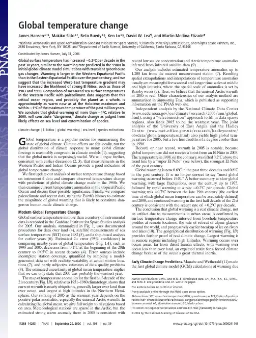
Global temperature changeJames Hansen*†‡,Makiko Sato*†,Reto Ruedy*§,Ken Lo*§,David W.Lea ¶,and Martin Medina-Elizade ¶*National Aeronautics and Space Administration Goddard Institute for Space Studies,†Columbia University Earth Institute,and §Sigma Space Partners,Inc.,2880Broadway,New York,NY 10025;and ¶Department of Earth Science,University of California,Santa Barbara,CA 93106Contributed by James Hansen,July 31,2006Global surface temperature has increased Ϸ0.2°C per decade in the past 30years,similar to the warming rate predicted in the 1980s in initial global climate model simulations with transient greenhouse gas changes.Warming is larger in the Western Equatorial Pacific than in the Eastern Equatorial Pacific over the past century,and we suggest that the increased West–East temperature gradient may have increased the likelihood of strong El Niños,such as those of 1983and parison of measured sea surface temperatures in the Western Pacific with paleoclimate data suggests that this critical ocean region,and probably the planet as a whole,is approximately as warm now as at the Holocene maximum and within Ϸ1°C of the maximum temperature of the past million years.We conclude that global warming of more than Ϸ1°C,relative to 2000,will constitute ‘‘dangerous’’climate change as judged from likely effects on sea level and extermination of species.climate change ͉El Niños ͉global warming ͉sea level ͉species extinctionsGlobal temperature is a popular metric for summarizing the state of global climate.Climate effects are felt locally,but the global distribution of climate response to many global climate forcings is reasonably congruent in climate models (1),suggesting that the global metric is surprisingly useful.We will argue further,consistent with earlier discussion (2,3),that measurements in the Western Pacific and Indian Oceans provide a good indication of global temperature change.We first update our analysis of surface temperature change based on instrumental data and compare observed temperature change with predictions of global climate change made in the 1980s.We then examine current temperature anomalies in the tropical Pacific Ocean and discuss their possible significance.Finally,we compare paleoclimate and recent data,using the Earth’s history to estimate the magnitude of global warming that is likely to constitute dan-gerous human-made climate change.Modern Global Temperature ChangeGlobal surface temperature in more than a century of instrumental data is recorded in the Goddard Institute for Space Studies analysis for 2005.Our analysis,summarized in Fig.1,uses documented procedures for data over land (4),satellite measurements of sea surface temperature (SST)since 1982(5),and a ship-based analysis for earlier years (6).Estimated 2error (95%confidence)in comparing nearby years of global temperature (Fig.1A ),such as 1998and 2005,decreases from 0.1°C at the beginning of the 20th century to 0.05°C in recent decades (4).Error sources include incomplete station coverage,quantified by sampling a model-generated data set with realistic variability at actual station loca-tions (7),and partly subjective estimates of data quality problems (8).The estimated uncertainty of global mean temperature implies that we can only state that 2005was probably the warmest year.The map of temperature anomalies for the first half-decade of the 21st century (Fig.1B ),relative to 1951–1980climatology,shows that current warmth is nearly ubiquitous,generally larger over land than over ocean,and largest at high latitudes in the Northern Hemi-sphere.Our ranking of 2005as the warmest year depends on the positive polar anomalies,especially the unusual Arctic warmth.In calculating the global mean,we give full weight to all regions based on area.Meteorological stations are sparse in the Arctic,but the estimated strong warm anomaly there in 2005is consistent withrecord low sea ice concentration and Arctic temperature anomalies inferred from infrared satellite data (9).Our analysis includes estimated temperature anomalies up to 1,200km from the nearest measurement station (7).Resulting spatial extrapolations and interpolations of temperature anomalies usually are meaningful for seasonal and longer time scales at middle and high latitudes,where the spatial scale of anomalies is set by Rossby waves (7).Thus,we believe that the unusual Arctic warmth of 2005is real.Other characteristics of our analysis method are summarized in Supporting Text ,which is published as supporting information on the PNAS web site.Independent analysis by the National Climate Data Center ( ͞oa ͞climate ͞research ͞2005͞ann ͞global.html),using a ‘‘teleconnection’’approach to fill in data sparse regions,also finds 2005to be the warmest year.The joint analysis of the University of East Anglia and the Hadley Centre ( ͞research ͞hadleycentre ͞obsdata ͞globaltemperature.html)also yields high global tem-perature for 2005,but a few hundredths of a degree cooler than in 1998.Record,or near record,warmth in 2005is notable,because global temperature did not receive a boost from an El Niño in 2005.The temperature in 1998,on the contrary,was lifted 0.2°C above the trend line by a ‘‘super El Niño’’(see below),the strongest El Niño of the past century.Global warming is now 0.6°C in the past three decades and 0.8°C in the past century.It is no longer correct to say ‘‘most global warming occurred before 1940.’’A better summary is:slow global warming,with large fluctuations,over the century up to 1975,followed by rapid warming at a rate Ϸ0.2°C per decade.Global warming was Ϸ0.7°C between the late 19th century (the earliest time at which global mean temperature can be accurately defined)and 2000,and continued warming in the first half decade of the 21st century is consistent with the recent rate of ϩ0.2°C per decade.The conclusion that global warming is a real climate change,not an artifact due to measurements in urban areas,is confirmed by surface temperature change inferred from borehole temperature profiles at remote locations,the rate of retreat of alpine glaciers around the world,and progressively earlier breakup of ice on rivers and lakes (10).The geographical distribution of warming (Fig.1B )provides further proof of real climate rgest warming is in remote regions including high latitudes.Warming occurs over ocean areas,far from direct human effects,with warming over ocean less than over land,an expected result for a forced climate change because of the ocean’s great thermal inertia.Early Climate Change Predictions.Manabe and Wetherald (11)madethe first global climate model (GCM)calculations of warming dueAuthor contributions:D.W.L.and M.M.-E.contributed data;J.H.,M.S.,R.R.,K.L.,D.W.L.,and M.M.-E.analyzed data;and J.H.wrote the paper.The authors declare no conflict of interest.Freely available online through the PNAS open access option.Abbreviations:SST,sea surface temperature;GHG,greenhouse gas;EEP,Eastern Equatorial Pacific;WEP,Western Equatorial Pacific;DAI,dangerous antrhopogenic interference;BAU,business as usual;AS,alternative scenario;BC,black carbon.‡Towhom correspondence should be addressed:E-mail:jhansen@.©2006by The National Academy of Sciences of the USA14288–14293͉PNAS ͉September 26,2006͉vol.103͉no.39 ͞cgi ͞doi ͞10.1073͞pnas.0606291103to instant doubling of atmospheric CO 2.The first GCM calculations with transient greenhouse gas (GHG)amounts,allowing compar-ison with observations,were those of Hansen et al.(12).It has been asserted that these calculations,presented in congressional testi-mony in 1988(13),turned out to be ‘‘wrong by 300%’’(14).That assertion,posited in a popular novel,warrants assessment because the author’s views on global warming have been welcomed in testimony to the United States Senate (15)and in a meeting with the President of the United States (16),at a time when the Earth may be nearing a point of dangerous human-made interference with climate (17).The congressional testimony in 1988(13)included a graph (Fig.2)of simulated global temperature for three scenarios (A,B,and C)and maps of simulated temperature change for scenario B.The three scenarios were used to bracket likely possibilities.Scenario A was described as ‘‘on the high side of reality,’’because it assumed rapid exponential growth of GHGs and it included no large volcanic eruptions during the next half century.Scenario C was described as ‘‘a more drastic curtailment of emissions than has generally been imagined,’’specifically GHGs were assumed to stop increasing after 2000.Intermediate scenario B was described as ‘‘the most plausi-ble.’’Scenario B has continued moderate increase in the rate of GHG emissions and includes three large volcanic eruptions sprin-kled through the 50-year period after 1988,one of them in the 1990s.Real-world GHG climate forcing (17)so far has followed a course closest to scenario B.The real world even had one large volcanic eruption in the 1990s,Mount Pinatubo in 1991,whereas scenario B placed a volcano in 1995.Fig.2compares simulations and observations.The red curve,as in ref.12,is the updated Goddard Institute for Space Studies observational analysis based on meteorological stations.The black curve is the land–ocean global temperature index from Fig.1,which uses SST changes for ocean areas (5,6).The land–ocean temper-ature has more complete coverage of ocean areas and yields slightly smaller long-term temperature change,because warming on aver-age is less over ocean than over land (Fig.1B ).Temperature change from climate models,including that re-ported in 1988(12),usually refers to temperature of surface air over both land and ocean.Surface air temperature change in a warming climate is slightly larger than the SST change (4),especially in regions of sea ice.Therefore,the best temperature observation for comparison with climate models probably falls between the mete-orological station surface air analysis and the land–ocean temper-ature index.Observed warming (Fig.2)is comparable to that simulated for scenarios B and C,and smaller than that for scenario A.Following refs.18and 14,let us assess ‘‘predictions’’by comparing simulated and observed temperature change from 1988to the most recent year.Modeled 1988–2005temperature changes are 0.59,0.33,and 0.40°C,respectively,for scenarios A,B,and C.Observed temper-ature change is 0.32°C and 0.36°C for the land–ocean index and meteorological station analyses,respectively.Warming rates in the model are 0.35,0.19,and 0.24°C per decade for scenarios A,B.and C,and 0.19and 0.21°C per decade for the observational analyses.Forcings in scenarios B and C are nearly the same up to 2000,so the different responses provide one measure of unforced variability in the model.Because of this chaotic variability,a 17-year period is too brief for precise assessment of model predictions,but distinction among scenarios and comparison with the real world will become clearer within a decade.Close agreement of observed temperature change with simula-tions for the most realistic climate forcing (scenario B)is accidental,given the large unforced variability in both model and real world.Indeed,moderate overestimate of global warming is likely because the sensitivity of the model used (12),4.2°C for doubled CO 2,is larger than our current estimate for actual climate sensitivity,which is 3Ϯ1°C for doubled CO 2,based mainly on paleoclimate data (17).More complete analyses should include other climate forcingsandFig.1.Surface temperature anomalies relative to 1951–1980from surface air measurements at meteorological stations and ship and satellite SST measurements.(A )Global annual mean anomalies.(B )Temperature anomaly for the first half decade of the 21stcentury.Annual Mean Global Temperature Change: ΔT s (°C)Fig.2.Global surface temperature computed for scenarios A,B,and C (12),compared with two analyses of observational data.The 0.5°C and 1°C tempera-ture levels,relative to 1951–1980,were estimated (12)to be maximum global temperatures in the Holocene and the prior interglacial period,respectively.Hansen et al.PNAS ͉September 26,2006͉vol.103͉no.39͉14289E N V I R O N M E N T A L S C I E N C EScover longer periods.Nevertheless,it is apparent that the first transient climate simulations (12)proved to be quite accurate,certainly not ‘‘wrong by 300%’’(14).The assertion of 300%error may have been based on an earlier arbitrary comparison of 1988–1997observed temperature change with only scenario A (18).Observed warming was slight in that 9-year period,which is too brief for meaningful comparison.Super El Niños.The 1983and 1998El Niños were successivelylabeled ‘‘El Niño of the century,’’because the warming in the Eastern Equatorial Pacific (EEP)was unprecedented in 100years (Fig.3).We suggest that warming of the Western Equatorial Pacific (WEP),and the absence of comparable warming in the EEP,has increased the likelihood of such ‘‘super El Niños.’’In the ‘‘normal’’(La Niña)phase of El Niño Southern Oscillation the east-to-west trade winds push warm equatorial surface water to the west such that the warmest SSTs are located in the WEP near Indonesia.In this normal state,the thermocline is shallow in the EEP,where upwelling of cold deep water occurs,and deep in the WEP (figure 2of ref.20).Associated with this tropical SST gradient is a longitudinal circulation pattern in the atmosphere,the Walker cell,with rising air and heavy rainfall in the WEP and sinking air and drier conditions in the EEP.The Walker circulation enhances upwelling of cold water in the East Pacific,causing a powerful positive feedback,the Bjerknes (21)feedback,which tends to maintain the La Niña phase,as the SST gradient and resulting higher pressure in the EEP support east-to-west trade winds.This normal state is occasionally upset when,by chance,the east-to-west trade winds slacken,allowing warm water piled up in the west to slosh back toward South America.If the fluctuation is large enough,the Walker circulation breaks down and the Bjerknes feedback loses power.As the east-to-west winds weaken,the Bjerknes feedback works in reverse,and warm waters move more strongly toward South America,reducing the thermocline tilt and cutting off upwelling of cold water along the South American coast.In this way,a classical El Niño is born.Theory does not provide a clear answer about the effect of global warming on El Niños (19,20).Most climate models yield either a tendency toward a more El Niño-like state or no clear change (22).It has been hypothesized that,during the early Pliocene,when the Earth was 3°C warmer than today,a permanent El Niño condition existed (23).We suggest,on empirical grounds,that a near-term global warming effect is an increased likelihood of strong El Niños.Fig.1B shows an absence of warming in recent years relative to 1951–1980in the equatorial upwelling region off the coast of South America.This is also true relative to the earliest period of SST data,1870–1900(Fig.3A ).Fig.7,which is published as supporting information on the PNAS web site,finds a similar result for lineartrends of SSTs.The trend of temperature minima in the East Pacific,more relevant for our purpose,also shows no equatorial warming in the East Pacific.The absence of warming in the EEP suggests that upwelling water there is not yet affected much by global warming.Warming in the WEP,on the other hand,is 0.5–1°C (Fig.3).We suggest that increased temperature difference between the near-equatorial WEP and EEP allows the possibility of increased temperature swing from a La Niña phase to El Niño,and that this is a consequence of global warming affecting the WEP surface sooner than it affects the deeper ocean.Fig.3B compares SST anomalies (12-month running means)in the WEP and EEP at sites (marked by circles in Fig.3A )of paleoclimate data discussed below.Absolute temperatures at these sites are provided in Fig.8,which is published as supporting information on the PNAS web site.Even though these sites do not have the largest warming in the WEP or largest cooling in the EEP,Fig.3B reveals warming of the WEP relative to the EEP [135-year changes,based on linear trends,are ϩ0.27°C (WEP)and Ϫ0.01°C (EEP)].The 1983and 1998El Niños in Fig.3B are notably stronger than earlier El Niños.This may be partly an artifact of sparse early data or the location of data sites,e.g.,the late 1870s El Niño is relatively stronger if averages are taken over Niño 3or a 5°ϫ10°box.Nevertheless,‘‘super El Niños’’clearly were more abundant in the last quarter of the 20th century than earlier in the century.Global warming is expected to slow the mean tropical circulation (24–26),including the Walker cell.Sea level pressure data suggest a slowdown of the longitudinal wind by Ϸ3.5%in the past century (26).A relaxed longitudinal wind should reduce the WEP–EEP temperature difference on the broad latitudinal scale (Ϸ10°N to 15°S)of the atmospheric Walker cell.Observed SST anomalies are consistent with this expectation,because the cooling in the EEP relative to WEP decreases at latitudes away from the narrower region strongly affected by upwelling off the coast of Peru (Fig.3A ).Averaged over 10°N to 15°S,observed warming is as great in the EEP as in the WEP (see also Fig.7).We make no suggestion about changes of El Niño frequency,and we note that an abnormally warm WEP does not assure a strong El Niño.The origin and nature of El Niños is affected by chaotic ocean and atmosphere variations,the season of the driving anomaly,the state of the thermocline,and other factors,assuring that there will always be great variability of strength among El Niños.Will increased contrast between near-equatorial WEP and EEP SSTs be maintained or even increase with more global warming?The WEP should respond relatively rapidly to increasing GHGs.In the EEP,to the extent that upwelling water has not been exposed to the surface in recent decades,little warming is expected,andtheBSST Change (°C) from 1870-1900 to 2001-2005Western and Eastern Pacific Temperature Anomalies (°C)parison of SST in West and East Equatorial Pacific Ocean.(A )SST in 2001–2005relative to 1870–1900,from concatenation of two data sets (5,6),as described in the text.(B )SSTs (12-month running means)in WEP and EEP relative to 1870–1900means.14290͉ ͞cgi ͞doi ͞10.1073͞pnas.0606291103Hansen etal.contrast between WEP and EEP may remain large or increase in coming decades.Thus,we suggest that the global warming effect on El Niños is analogous to an inferred global warming effect on tropical storms (27).The effect on frequency of either phenomenon is unclear,depending on many factors,but the intensity of the most powerful events is likely to increase as GHGs increase.In this case,slowing the growth rate of GHGs should diminish the probability of both super El Niños and the most intense tropical storms.Estimating Dangerous Climate ChangeModern vs.Paleo Temperatures.Modern SST measurements (5,6)are compared with proxy paleoclimate temperature (28)in the WEP (Ocean Drilling Program Hole 806B,0°19ЈN,159°22ЈE;site circled in Fig.3A )in Fig.4A .Modern data are from ships and buoys for 1870–1981(6)and later from satellites (5).In concatenation of satellite and ship data,as shown in Fig.8A ,the satellite data are adjusted down slightly so that the 1982–1992mean matches the mean ship data for that period.The paleoclimate SST,based on Mg content of foraminifera shells,provides accuracy to Ϸ1°C (29).Thus we cannot be sure that we have precisely aligned the paleo and modern temperature scales.Accepting paleo and modern temperatures at face value implies a WEP 1870SST in the middle of its Holocene range.Shifting the scale to align the 1870SST with the lowest Holocene value raises the paleo curve by Ϸ0.5°C.Even in that case,the 2001–2005WEPSST is at least as great as any Holocene proxy temperature at that location.Coarse temporal resolution of the Holocene data,Ϸ1,000years,may mask brief warmer excursions,but cores with higher resolution (29)suggest that peak Holocene WEP SSTs were not more than Ϸ1°C warmer than in the late Holocene,before modern warming.It seems safe to assume that the SST will not decline this century,given continued increases of GHGs,so in a practical sense the WEP temperature is at or near its highest level in the Holocene.Fig.5,including WEP data for the past 1.35million years,shows that the current WEP SST is within Ϸ1°C of the warmest intergla-cials in that period.The Tropical Pacific is a primary driver of the global atmosphere and ocean.The tropical Pacific atmosphere–ocean system is the main source of heat transported by both the Pacific and Atlantic Oceans (2).Heat and water vapor fluxes to the atmosphere in the Pacific also have a profound effect on the global atmosphere,as demonstrated by El Niño Southern Oscillation climate variations.As a result,warming of the Pacific has worldwide repercussions.Even distant local effects,such as thinning of ice shelves,are affected on decade-to-century time scales by subtropical Pacific waters that are subducted and mixed with Antarctic Intermediate Water and thus with the Antarctic Circumpolar Current.The WEP exhibits little seasonal or interannual variability of SST,typically Ͻ1°C,so its temperature changes are likely to reflect large scale processes,such as GHG warming,as opposed to small scale processes,such as local upwelling.Thus,record Holocene WEP temperature suggests that global temperature may also be at its highest level.Correlation of local and global temperature change for 1880–2005(Fig.9,which is published as supporting information on the PNAS web site)confirms strong positive correlation of global and WEP temperatures,and an even stronger correlation of global and Indian Ocean temperatures.The Indian Ocean,due to rapid warming in the past 3–4decades,is now warmer than at any time in the Holocene,independent of any plausible shift of the modern temperature scale relative to the paleoclimate data (Fig.4C ).In contrast,the EEP (Fig.4B )and perhaps Central Antarctica (Vostok,Fig.4D )warmed less in the past century and are probably cooler than their Holocene peak values.However,as shown in Figs.1B and 3A ,those are exceptional regions.Most of the world and the global mean have warmed as much as the WEP and Indian Oceans.We infer that global temperature today is probably at or near its highest level in the Holocene.Fig.5shows that recent warming of the WEP has brought its temperature within Ͻ1°C of its maximum in the past million years.There is strong evidence that the WEP SST during the penultimate interglacial period,marine isotope stage (MIS)5e,exceeded the WEP SST in the Holocene by 1–2°C (30,31).This evidence is consistent with data in Figs.4and 5and with our conclusion that the Earth is now within Ϸ1°C of its maximum temperature in the past million years,because recent warming has lifted the current temperature out of the prior Holocenerange.parison of modern surface temperature measurements with paleoclimate proxy data in the WEP (28)(A ),EEP (3,30,31)(B ),Indian Ocean (40)(C ),and Vostok Antarctica (41)(D).Fig.5.Modern sea surface temperatures (5,6)in the WEP compared with paleoclimate proxy data (28).Modern data are the 5-year running mean,while the paleoclimate data has a resolution of the order of 1,000years.Hansen et al.PNAS ͉September 26,2006͉vol.103͉no.39͉14291E N V I R O N M E N T A L S C I E N C ESCriteria for Dangerous Warming.The United Nations FrameworkConvention on Climate Change (www.unfccc.int)has the objective ‘‘to achieve stabilization of GHG concentrations’’at a level pre-venting ‘‘dangerous anthropogenic interference’’(DAI)with cli-mate,but climate change constituting DAI is undefined.We suggest that global temperature is a useful metric to assess proximity to DAI,because,with knowledge of the Earth’s history,global tem-perature can be related to principal dangers that the Earth faces.We propose that two foci in defining DAI should be sea level and extinction of species,because of their potential tragic consequences and practical irreversibility on human time scales.In considering these topics,we find it useful to contrast two distinct scenarios abbreviated as ‘‘business-as-usual’’(BAU)and the ‘‘alternative scenario’’(AS).BAU has growth of climate forcings as in intermediate or strong Intergovernmental Panel on Climate Change scenarios,such as A1B or A2(10).CO 2emissions in BAU scenarios continue to grow at Ϸ2%per year in the first half of this century,and non-CO 2positive forcings such as CH 4,N 2O,O 3,and black carbon (BC)aerosols also continue to grow (10).BAU,with nominal climate sensitivity (3Ϯ1°C for doubled CO 2),yields global warming (above year 2000level)of at least 2–3°C by 2100(10,17).AS has declining CO 2emissions and an absolute decrease of non-CO 2climate forcings,chosen such that,with nominal climate sensitivity,global warming (above year 2000)remains Ͻ1°C.For example,one specific combination of forcings has CO 2peaking at 475ppm in 2100and a decrease of CH 4,O 3,and BC sufficient to balance positive forcing from increase of N 2O and decrease of sulfate aerosols.If CH 4,O 3,and BC do not decrease,the CO 2cap in AS must be lower.Sea level implications of BAU and AS scenarios can be consid-ered in two parts:equilibrium (long-term)sea level change and ice sheet response time.Global warming Ͻ1°C in AS keeps tempera-tures near the peak of the warmest interglacial periods of the past million years.Sea level may have been a few meters higher than today in some of those periods (10).In contrast,sea level was 25–35m higher the last time that the Earth was 2–3°C warmer than today,i.e.,during the Middle Pliocene about three million years ago (32).Ice sheet response time can be investigated from paleoclimate evidence,but inferences are limited by imprecise dating of climate and sea level changes and by the slow pace of weak paleoclimate forcings compared with stronger rapidly increasing human-made forcings.Sea level rise lagged tropical temperature by a few thousand years in some cases (28),but in others,such as Meltwater Pulse 1A Ϸ14,000years ago (33),sea level rise and tropical temperature increase were nearly synchronous.Intergovernmental Panel on Climate Change (10)assumes negligible contribution to 2100sea level change from loss of Greenland and Antarctic ice,but that conclusion is implausible (17,34).BAU warming of 2–3°C would bathe most of Greenland and West Antarctic in melt-water during lengthened melt seasons.Multiple positive feedbacks,in-cluding reduced surface albedo,loss of buttressing ice shelves,dynamical response of ice streams to increased melt-water,and lowered ice surface altitude would assure a large fraction of the equilibrium ice sheet response within a few centuries,at most (34).Sea level rise could be substantial even in the AS,Ϸ1m per century,and cause problems for humanity due to high population in coastal areas (10).However,AS problems would be dwarfed by the disastrous BAU,which could yield sea level rise of several meters per century with eventual rise of tens of meters,enough to transform global coastlines.Extinction of animal and plant species presents a picture anal-ogous to that for sea level.Extinctions are already occurring as a result of various stresses,mostly human-made,including climate change (35).Plant and animal distributions are a reflection of the regional climates to which they are adapted.Thus,plants and animals attempt to migrate in response to climate change,but theirpaths may be blocked by human-constructed obstacles or natural barriers such as coastlines.A study of 1,700biological species (36)found poleward migration of 6km per decade and vertical migration in alpine regions of 6m per decade in the second half of the 20th century,within a factor of two of the average poleward migration rate of surface isotherms (Fig.6A )during 1950–1995.More rapid warming in 1975–2005yields an average isotherm migration rate of 40km per decade in the Northern Hemisphere (Fig.6B ),exceeding known paleoclimate rates of change.Some species are less mobile than others,and ecosystems involve interactions among species,so such rates of climate change,along with habitat loss and fragmentation,new invasive species,and other stresses are expected to have severe impact on species survival (37).The total distance of isotherm migration,as well as migration rate,affects species survival.Extinction is likely if the migration distance exceeds the size of the natural habitat or remaining habitat fragment.Fig.6shows that the 21st century migration distance for a BAU scenario (Ϸ600km)greatly exceeds the average migration distance for the AS (Ϸ100km).It has been estimated (38)that a BAU global warming of 3°C over the 21st century could eliminate a majority (Ϸ60%)of species on the planet.That projection is not inconsistent with mid-century BAU effects in another study (37)or scenario sensitivity of stress effects (35).Moreover,in the Earth’s history several mass extinc-tions of 50–90%of species have accompanied global temperature changes of Ϸ5°C (39).We infer that even AS climate change,which would slow warming to Ͻ0.1°C per decade over the century,would contribute to species loss that is already occurring due to a variety of stresses.However,species loss under BAU has the potential to be truly disastrous,conceivably with a majority of today’s plants and animals headed toward extermination.DiscussionThe pattern of global warming (Fig.1B )has assumed expected characteristics,with high latitude amplification and larger warming over land than over ocean,as GHGs have become the dominant climate forcing in recent decades.This pattern results mainly from the ice–snow albedo feedback and the response times of ocean andland.Fig.6.Poleward migration rate of isotherms in surface observations (A and B )and in climate model simulations (17)for 2000–2100for Intergovernmental Panel on Climate Change scenario A2(10)and an alternative scenario of forcings that keeps global warming after 2000less than 1°C (17)(C and D ).Numbers in upper right are global means excluding the tropical band.14292͉ ͞cgi ͞doi ͞10.1073͞pnas.0606291103Hansen etal.。

Climate Change演讲稿引言大家好,我要和大家谈论的话题是气候变化。
气候变化是一个全球性的问题,对我们每个人都有着深远的影响。
今天,我想和大家一起探讨气候变化的原因、影响以及应对措施。
气候变化的原因气候变化主要是由人类活动引起的。
工业化、交通运输、森林砍伐等行为导致了大量温室气体的排放。
温室气体的增加导致了地球的温度升高,气候的变化变得异常剧烈。
气候变化的影响气候变化对我们的生活和生态系统造成了严重的影响。
首先,全球变暖导致了极端天气事件的增加,如台风、洪水、干旱等。
这些天气事件给人们的生活和财产带来了巨大的损失。
其次,气候变化还威胁到了许多动植物的生存。
生物多样性正在遭受破坏,这对生态平衡和人类的生存都是巨大的挑战。
应对气候变化的措施为了应对气候变化,我们需要采取行动。
首先,我们应该致力于减少温室气体的排放。
这可以通过使用清洁能源、加强能源效率、减少汽车尾气排放等方式实现。
其次,我们还需要加强对气候变化的监测和预警,及时采取行动减轻灾害的影响。
最后,我们需要加强国际合作,共同应对气候变化。
各国应共同努力,制定和执行全球性的减排目标,推动实现可持续发展。
结论气候变化是人类面临的重大挑战,我们每个人都应该意识到自己的责任。
通过减少温室气体的排放和积极应对气候变化,我们可以为未来的世界创造一个更美好的环境。
让我们共同行动起来,保护我们的地球,为后代创造一个可持续的未来。
谢谢大家!---*请注意,以上内容仅供参考,具体演讲稿可以根据需要进行修改。
*。


Tackle Climate Change Actively and Promote Sustainable Development--Speech at the EastWest Institute Seminar by H.E. Ambassador Song Zhe, Head of the Mission of the P.R.China to the EU 16 February 2010Ladies and Gentlemen:I am very pleased to be at this meeting and exchange views with you. I would like to take this opportunity to make three points: first, the Copenhagen Conference was a new starting point to tackle climate change; Secondly, the international community should give adequate attention to the issue of adaptation; Thirdly, China and the EU should strengthen dialogue and cooperation on climate change.We still have fresh memories of the Copenhagen Conference which was held two months ago. Although the meeting experienced twists and turns, but thanks to the joint efforts of all parties, it ultimately obtained two important results. First, by adhering to the United Nations Framework Convention on Climate Change, the Kyoto Protocol and the Bali road map, the conference identified clearly the direction for the negotiations in the next step; Secondly, the conference issued the Copenhagen Accord, marking new progress in terms of binding reduction by developed countries and voluntary action by developing countries. It also reached certain consensus on issues such as long-term goals, funding, technology and transparency, which laid the foundation for further strengthening international cooperation on climate change and gave political impetus to future negotiations. It is fair to say that the Copenhagen conference was a success. It produced the best result that can be achieved at this stage, which should be cherished.On tackling climate change, the road is long and tortuous. The Copenhagen Conference is not the end, but a new beginning. In recent weeks, there are nearly one hundred countries which notified the Secretariat of the Copenhagen Accord their respective emission reduction or mitigation targets.A series of important international conferences will be held in Bonn and Mexico this year. As a responsible member of the international community, China will continue to play an active and constructive role, earnestly fulfill its commitment, strengthen international cooperation, and with the Copenhagen Accord as the basis, work together with other parties for an early conclusion of the "Bali road map", so as to promote continuous progress of the international cooperation on climate change.Recently, Chinese Premier Wen Jiabao sent letters to Danish Prime Minister Rasmussen and UN Secretary-General Ban Ki-moon and stated that China supports the Copenhagen Accord. Premier Wen reiterates that China will strive to achieve national voluntary reduction targets, that is, by 2020, carbon dioxide emissions per unit of GDP will drop by 40% to 45% than 2005, non-fossil energy will account for about 15% of primary energy consumption, forest area will increase by 40 million hectares over 2005 and forest carbon sink by 1.3 billion cubic meters. This is a voluntary action China takes according to its own national conditions and stage of development, it is not attached to any conditions, or links to other country's emission reduction targets. It reflects the maximum efforts that the Chinese government can make.Here, I would like to highlight that China is still a developing country. It is in the critical stage of rapid development of industrialization and urbanization. We are facing an arduous task of economic development and improving people's livelihood. China's per capita GDP ranks after the world's first 100. By the UN standard, 150 million Chinese remain in poverty. Every year jobs for 12 million people need to be created, even more than the entire population of Belgium. In addition,China's coal-dominated energy mix poses special difficulties to emission reduction.Even so, the Chinese Government has always taken a responsible attitude towards the nation and mankind, and takes climate change as an important strategic task. To use a metaphor, we want mountains of gold and silver, but first of all we want mountains of trees. China will not repeat the model of "pollution first, treatment later" as it was in the history of the developed countries. China will set its own mitigation targets as compulsory targets of the national economic and social development plan and make efforts to meet our committed targets and do even more. We will unswervingly pursue sustainable development and honor our commitment by taking concrete actions.Ladies and gentlemen,Mitigation and adaptation are two integral aspects in tackling climate change. Mitigation is a relatively longer-term and challenging task, whereas adaptation is more immediate and urgent. The core of adaptation is funding. The UNFCCC explicitly stipulates the obligation on the part of developed countries to provide funding and technology to developing countries. At present, the international community has established a number of multilateral financing mechanisms, including the Least Developed Countries Fund. But frankly speaking, the international community's emphasis on adaptation is far from enough. The funds that are available and can really be put in place by the existing mechanisms are very limited, and falling far short of the actual needs and expectations from the developing countries.The international community should give more attention to adaptation. It's been wrong that we put so much emphasis on mitigation but so little on adaptation. The developed countries, in particular, should shoulder the responsibility, and in accordance with the Convention, deliver their promises to developing countries on financial and technology support. The Copenhagen Conference, having reached a preliminary consensus on the issue of funding, represented a step in the right direction. However, the Accord does not clearly specify the sources of funding in the short term or how they are going to be implemented. Neither does it stipulate the exact amount of long-term funding commitment of the countries concerned. There leaves much uncertainty. We hope that the developed countries will demonstrate political sincerity and take concrete action to fulfill its obligations, rather than evading or shifting to others their responsibilities.Ladies and gentlemen,China-EU cooperation on climate change is already a long story. As early as in 2005, the two sides established partnership on climate change. At the 12th China-EU Summit last year, the two sides decided to upgrade such partnership and strengthen policy dialogue and practical cooperation in the field of climate change. Following the Copenhagen Conference, the two sides plan to add an extra round of consultations on climate change which will take place in the near future. The EU possess advanced concepts and technologies in the field of energy saving and environmental protection. China has a vast market demand. The two sides should further tap the potentials for cooperation on energy and climate change, especially in the following areas:First, energy conservation and energy efficiency. China's energy utilization efficiency is far lower than the EU and other developed countries, and China needs to further reduce carbon dioxide emissions per unit of GDP.The second area is renewable energy. By cooperation under the Clean Development Mechanism,the EU could help China to promote renewable energy development, improve energy structure, and strengthen social environmental awareness.The third area is clean energy. For quite a long time in the future, China's energy production and consumption will continue to be dominated by coal, which present us a vast platform for technical cooperation.Ladies and Gentlemen:The EU is the world's biggest economy, and China is the world's biggest developing country. To strengthen practical cooperation between China and the EU on climate change, and sustainable development not only serves the fundamental interests of both sides, but is also conducive to world prosperity and development. We are willing to cooperate with all communities in the EU and make unremitting efforts to cope with climate change and achieve sustainable development. Thank you!。
MP R AMunich Personal RePEc ArchiveModelling Agricultural Production Risk and the Adaptation to Climate Change Finger,Robert and Schmid,St´e phanieETH Z¨u richJuly2007Online at http://mpra.ub.uni-muenchen.de/3943/ MPRA Paper No.3943,posted07.November2007/03:34M ODELING A GRICULTURAL P RODUCTION R ISK AND THE A DAPTATION TOC LIMATE C HANGER OBERT F INGER1, S TÉPHANIE S CHMID21Institute for Environmental Decisions, ETH Zurich, Switzerland2 Agroscope Reckenholz-Tänikon Research Station ART, Zürich, Switzerlandrofinger@ethz.chPaper prepared for presentation at the 101st EAAE Seminar ‘Management of Climate Risks in Agriculture’, Berlin, Germany, July 5-6, 2007Copyright 2007 by Robert Finger and Stéphanie Schmid. All rights reserved. Readers may make verbatim copies of this document for non-commercial purposes by any means, provided that this copyright notice appears on all such copies.1M ODELING A GRICULTURAL P RODUCTION R ISK AND THE A DAPTATION TOC LIMATE C HANGERobert Finger, Stéphanie Schmid∗AbstractA model that integrates biophysical simulations in an economic model is used to analyze the impact of climate change on crop production. The biophysical model simulates future plant-management-climate relationships and the economic model simulates farmers’ adaptation actions to climate change using a nonlinear programming approach. Beyond the development of average yields, special attention is devoted to the impact of climate change on crop yield variability.This study analyzes corn and winter wheat production on the Swiss Plateau with respect to climate change scenarios that cover the period of 2030-2050. In our model, adaptation options such as changes in seeding dates, changes in production intensity and the adoption of irrigation farming are considered. Different scenarios of climate change, output prices and farmers’ risk aversion are applied in order to show the sensitivity of adaptation strategies and crop yields, respectively, on these factors.Our results show that adaptation actions, yields and yield variation highly depend on both climate change and output prices. The sensitivity of adaptation options and yields, respectively, to prices and risk aversion for winter wheat is much lower than for corn because of different growing periods. In general, our results show that both corn and winter wheat yields increase in the next decades. In contrast to other studies, we find the coefficient of variation of corn and winter wheat yields to decrease. We therefore conclude that simple adaptation measures are sufficient to take advantage of climate change in Swiss crop farming. Keywordsclimate change, robust estimation, yield variation, corn, winter wheat, market liberalization1 IntroductionIn the next decades Swiss farmers will face changing climatic conditions, which are characterized by elevated carbon dioxide concentrations, reduced summer rainfalls and elevated temperatures for the Swiss Plateau region (O C CC,2005). Furthermore, Swiss agriculture will face changing market conditions due to market liberalization. Both input and output prices are expected to decrease in the next decades. The goal of this paper is to assess ∗Robert Finger (Institute for Environmental Decisions, ETH Zürich), Dr. Stéphanie Schmid (Agroscope Reckenholz-Tänikon Research Station ART, Zürich). This work was supported by the Swiss National Science Foundation in the framework of the National Centre of Competence in Research on Climate (NCCR Climate). We would like to thank Werner Hediger for helpful comments..2impacts of climate and price changes on Swiss corn (Zea mays L.) and winter wheat (Triticum L.) production.Previous studies that analyzed the effects of climate change (CC) on crop production and crop variability were either based on (crop) simulation or regression models. Crop simulation models simulate and compare crop productivity for different climatic conditions (e.g. T ORRIANI ET AL.,2007a). Regression models use historical climate and agricultural data to outline potential effects of climate change on crop productivity (e.g. I SIK AND D EVADOSS, 2006). Both approaches are not sufficient to analyze all aspects of impacts of CC on crop production (A NTLE AND C APALBO,2001). If the analysis is restricted to crop physiology, such as in crop simulations, farmer’s adaptation actions are not taken into account. But, sufficient inference requires consideration of farmers’ reactions to changes in climate and economic conditions. This contrasts the extrapolation of historical farm-level and aggregated data that takes into account farmers’ historical reactions to changes in climatic and economic conditions. However, historical data is not able to capture future plant-climate interactions in a sufficient manner, in particular if the crop-weather relationship is restricted to a few variables such as temperature and rainfall. Moreover, such models cannot sufficiently integrate expected CO2 fertilization effects on plants due to low variation in historical CO2 concentrations (A NTLE AND C APALBO,2001). In order to overcome these drawbacks, we use a combination of both approaches, simulation of future crop productivity and regression models.Existing studies show that CC will have particular influence on yield variation (M EARNS ET AL.,1996,T UBIELLO ET AL.,2000,S OUTHWORTH ET AL.,2002,F UHRER,2003,C IAIS ET AL., 2005, and, T ORRIANI ET AL.,2007a). The analysis of yield variation was restricted on climatic variables such as shifts in annual means and intra-annual distributions of climatic variables. These studies do not take adaptation actions of the farmers into account. In contrast, our approach considers farmers’ adaptation actions to CC and is thus more sufficient to model the impact of CC on yield variation. An empirical example for corn and winter wheat production on the Swiss Plateau is used to asses the impact of CC on both crop yields and yield variability.Our model covers no short term adaptation actions (i.e. tactical decisions) of farmers, but adaptation choices with a longer time horizon, i.e. strategic and structural decisions (cp. R ISBEY ET AL.,1999). We consider strategic and structural decisions that consist of changes in production intensity, changes in seeding dates and the adoption of irrigation farming. Even though crop yields are influenced by various factors, our analysis is restricted on the crucial inputs nitrogen fertilizer and irrigation water. Thus, the analysis is of particular environmental and economic interest because application of both inputs can lead to the degradation of environmental systems (IEEP, 2000, and, K HANNA ET AL.,2000). Nitrogen fertilizer is furthermore a major source of climate relevant agricultural emissions (H UNGATE ET AL., 2003).Our model is based on an integrated assessment approach that integrates a biophysical in an economic model. In contrast to other integrated models (e.g. A NTLE AND C APALBO,2001), farmers’ behavior is simulated using nonlinear programming. The model is divided into three major parts: data simulation, estimation of model parameters and economic simulation. Data simulation describes the yield simulation process which includes the experimental design that enhances yield variability with respect to nitrogen fertilizer and irrigation. Furthermore, current and simulated future daily weather data are crucial inputs for the simulation process. The data simulation results in individual datasets for each climatic scenario and crop that contain yield and input data. These datasets are used to estimate production and yield variation functions, respectively. Subsequently, based on these functions, farmers’ adaptation choices under different climate, price and risk aversion scenarios are simulated using nonlinear programming. Final assessment is based on a comparison of optimal input levels3and consequential yield levels, yield variation, coefficients of variation and utility of quasi-rents for these scenarios of climate change, future prices and risk aversion.In Section 2, 3 and 4, the data simulation, the economic model and the estimation processes are described, respectively. Estimation and economic simulation results are presented in Section 5 and 6, respectively. A final discussion of the impact of climate change on Swiss corn and winter wheat production is given in the concluding Section 7.2 Crop yield simulation and dataOur analysis is based on yield data generated by the deterministic crop yield simulation model CropSyst (e.g. S TÖCKLE ET AL.,2003). This is a process-based, multi-crop, multi-year cropping system simulation model. The model simulates above- and belowground processes of a single land block fragment representing a biophysically homogenous area. The model processes are simulated on a daily time step. They comprise the soil water budget, soil-plant nitrogen budget, crop phenology, canopy and root growth, biomass production, crop yield, residue production and decomposition, and soil erosion by water. These processes are simulated in response to weather, soil characteristics, crop characteristics, and management options. The model is therefore highly suitable to analyze the impact of environment and management on crop productivity, and has already been tested for a wide range of environmental conditions (e.g. D ONATELLI ET AL.,1997, and,S TÖCKLE ET AL.,2003). T ORRIANI ET AL. (2007a) provide a model calibration, tests of yield simulation and a documentation of critical crop parameters of corn and winter wheat for the Swiss Plateau that are used in our yield simulation. In general, the comparability of simulated and observed yields is restricted because the simulations do not account for yield reducing events such as hail, disease and insect infestation.CropSyst requires daily values of maximum and minimum temperature, solar radiation, and maximum and minimum relative humidity. In CropSyst, phenology is determined by thermal time, i.e., a specific development stage is reached when the required daily accumulation of average air temperature above a base temperature and below a cutoff temperature is reached. Daily climate input as required by CropSyst is obtained from the monitoring network of the Swiss Federal Office of Meteorology and Climate (MeteoSwiss). We use data from six meteorological stations distributed over the Swiss Plateau ranging from 06°57' to 08°54' longitude (F INGER AND S CHMID,2007). To simulate current climate conditions, we use climate data of the years 1981 to 2003. Compared to an approach with one single location, the use of observations from six different weather stations broadens the data base. For the atmospheric CO2 concentration input we use recordings from the years 1981 to 2003. They range from 339 ppm to 379 ppm (S CHRÖTER ET AL.,2005).Two climate change scenarios are applied to generate crop production functions for the coming decades. Climate scenarios with projections for the years 2030 and 2050 were taken from O C CC (2005). OcCC climate projections are based on simulations with two CO2 emission scenarios, four global climate models, and eight regional climate models. These simulations with totally 16 scenario-model combinations on a grid of 50x50 km over the whole European continent were performed within the scope of the PRUDENCE project (C HRISTENSEN ET AL., 2001). The OcCC climate projections used in this study represent the median of the simulations with the 16 scenario-model combinations for the years 2030 and 2050. The scenarios are abbreviated in the following as 2030 and 2050. The baseline for these climate anomalies is the year 1990. They include seasonal changes of temperature and precipitation for northern Switzerland (Table 1).4Table 1: Seasonal anomalies of temperature and precipitation2030 2050 DJF MAM JJA SON DJF MAM JJA SON Temperature + 1 + 0.9 + 1.4 + 1.1 +1.8 +1.8 +2.7 +2.1Precipitation 1.04 1.00 0.91 0.97 1.08 0.99 0.83 0.94*) Anomalies of temperature in °C (absolute value) and of precipitation in relative values with respect to the climate of the year 1990. DJF: December-February; MAM: March-May; JJA: June-August; SON: September-November.Source: O C CC (2005)Based on today’s weather data and the anomalies of temperature and precipitation (Table 1), a set of climate data are generated for each of the climate change scenarios using the stochastic weather generator LARS-WG (S EMENOV AND B ARROW,1998). To achieve monthly anomalies as required by LARS-WG, the seasonal anomalies are linearly interpolated. For the 2030 scenario, the CO2 concentrations (IPCC, 2000) range from 437 ppm to 475 ppm. For the 2050 scenario, CO2 concentrations in the range of 495 ppm to 561 ppm are assumed. Within the simulation years, the atmospheric CO2 concentration is varied randomly within the defined range.For each location and scenario, the same soil type is assumed. It follows T ORRIANI ET AL. (2007a) where this soil is used to calibrate the CropSyst model for Switzerland. The soil texture is characterized with 38% clay, 36% silt, and 26% sand. Based on the texture, CropSyst assesses the hydraulic properties of the soil. Soil depth amounts to 1.5 m and the soil organic matter content is at 2.6% weight in the top soil layer (5 cm) and 2.0% in lower soil layers.The applied management scenarios are uniform on the simulated crop area and include nitrogen (N) fertilization and irrigation. The amount of N applied per year ranged between 0 and 320 kg ha-1 for corn and between 0 and 360 kg ha-1 for winter wheat. Currently applied amounts of N fertilizer (W ALTHER ET AL.,2001) are expanded in the simulation in order to cover potential future N fertilization strategies. For corn (winter wheat), there are three fertilizer applications per year if N≤160 kg ha-1(N≤180 kg ha-1) and four fertilizer applications per year if N>160 kg ha-1 (N>180 kg ha-1), respectively, as shown in Table 2. For higher N amounts, however, an additional application date is introduced between the second and third date. In the simulations, fertilizer application dates are defined relative to the seeding date and derived from D UBOIS ET AL. (1998) and W ALTHER ET AL. (2001).Table 2: Distribution of annual fertilizer amountsDistribution of annual fertilizer [kgN ha-1]to the dates of applicationCorn up to 160 kg: 1 : 1 : 0 : 2 up to 320 kg: 1 : 1 : 1 : 2Winter Wheat up to 180 kg: 6 : 7 : 0 : 5 up to 360 kg: 6 : 7 : 5 : 5To simulate irrigation, we chose the automatic irrigation option of CropSyst. With this option, irrigation is triggered as soon as soil moisture is lower than a specific user-defined value. The degree of soil moisture is expressed as a value between 0 (permanent wilting point) and 1 (field capacity). When soil moisture falls below the previously defined value, water is added to the soil until field capacity is reached. However, there is an upper limit of irrigation water of 20 mm per irrigation event. Irrigation starts one day after seed and ends on the day of56harvest. The simulated experimental framework is equal for each climate scenario. This allows for comparability of results.For simulations under current climate we use seeding dates provided by D UBOIS ET AL . (1999) and T ORRIANI ET AL . (2007a). The temperature increase under the climate change scenarios leads to a shift of the annual temperature pattern and thus to a shift of the period of optimal crop development (T ORRIANI ET AL ., 2007a). Therefore, seeding dates are placed according to the temperature offset of the climate change scenario (Table 3). Even though seeding dates are placed earlier, CC leads to shorter maturity periods. Thus, shifts in average dates of maturity, which are equal to dates of harvest, are larger than for seeding dates (Table 3).Table 3: Seeding and average harvesting dates for the applied climate scenarios. Climate Scenario Current climate 2030 2050 th th th Corn Average Day of Maturity (Harvest)17th September (263) 4th September (250) 28th August (240) th th th Winter Wheat Average Day of Maturity (Harvest)05th August (217) 27th July (208) 18th July (199) *) Numbers in brackets are days of year.Source: CropSyst Simulations.For each location and year one simulation is conducted without application of fertilizer and irrigation. Furthermore, to broaden variability, the amount of fertilizer and the degree of soil moisture that triggers irrigation was varied randomly within the defined range. The datasets contain, depending on the crop and climate scenario, between 527 and 541 observations. A dry matter content of 85% and 90% is assumed for corn and winter wheat yields, respectively. 3 The economic modelOur analysis is based on utility-maximization with expected utility E(U) defined as follows:∫∞=0)()())((ππππd f U U E(1)Where E is the expectation operator and )(πU is the utility of quasi-rents π (revenue minus variable costs). The latter is treated as a random variable with density function )(πf . The stochastic character of quasi-rents can be the result of both stochastic yields and stochastic prices. Input and output prices are assumed to be deterministic in our analysis. Only crop yields are stochastic, with yield variation y σ. Production and yield variation functions are assumed to be known. Yield variation is therefore treated as risk and not as uncertainty. Risk preferences are incorporated with a preference parameter towards variation of quasi-rents (πσ). The utility function, which is linear in quasi-rents, is defined as follows (following H AZELL AND N ORTON , 1986):πγσππ−=)()(E U (2)Where γ is the coefficient of risk aversion (defined as )//()/(πσπ∂∂∂∂−U U ) which indicates risk-averse, risk-neutral and risk-taking behavior if 0>γ, 0=γ, and 0<γ, respectively.An indicator function, I , is used to model farmers’ adoption of irrigation farming: 1=I for adoption of an irrigation system and 0=I for crop farming without irrigation. Farmers are7 assumed to implement an irrigation system if expected utility minus adoption costs is higher than expected utility of crop farming without application of irrigation. That is, 1=I iff ()())()(01==>−I I U E K U E ππ, where K are the variable costs of adoption, e.g. the rental costs of the irrigation system. Expected quasi-rent )(πE is defined asIK ZX X y pE E −−=))(()(π (3)Where y(X) denotes the functional relationship, i.e. production function, between output scalar (y) and the vector of inputs (X), p the output price scalar and Z an input price vector. The input vector consist of two inputs: nitrogen (N ) and irrigation water (W ). The decision on adoption of irrigation farming leads to two types of production functions in this model: one with and one without irrigation, respectively. This distinction is omitted in this section to ensure lucidity. The standard deviation of quasi-rent is defined as:))(((ππσπE E −= (4)Under assumption of deterministic prices and by rearrangement of (4), the standard deviation of quasi-rent simplifies to y p σσπ=. Expected yields (i.e. solutions on the production function) are used to derive yield variation, )(X y σ. The latter is defined as the absolute difference between observed yields (i.e. simulated observations) and expected yields (eqn. 5). )(()()(X y E X y X y −=σ (5)Therefore, the difference between observed and predicted yields for observation i is the absolute residual of the regression analysis, i e , i.e. )()()(i i i i i i yi X y X y e X −==σ. Yield variation is determined by weather and soil conditions and input use, ),()(N W I f X y ⋅=σ. In this model, the intercept captures weather and soil effects on yield variability. Irrigation water is part of yield variation functions only for irrigation farming, i.e. 1=I . Substitution of eqn. (3) and (5) in (2) leads to the following final optimization problem:()IK X p ZX X y pE U E y y X −−−=)())(()(max ,σγπ (6)Expected utility (eqn. 6) is maximized subject to the production function constraint y(X). The first order condition for utility maximization is presented in section 6.4 Estimation methodology and functional formsThe production function, )(X f y =, is fitted to a square root functional form (eqn. 7), following F INGER AND H EDIGER (2007).1/21/21/2012345()Y N I W N I W I N W αααααα=+⋅+⋅⋅+⋅+⋅⋅+⋅⋅⋅ (7)Y denotes corn yield in kilogram, N the amount of nitrogen applied (kg ha -1), and W irrigation water applied in mm. The αi ’s are parameters that must satisfy the subsequent conditions in order to ensure decreasing marginal productivity of each input factor: 12,0αα> and 34,0αα<. If 50α>, the two input factors are complementary. They are competitive if 50α<, while 50α= indicates independence of the two input factors.The estimation of model parameters is a two step procedure that is described in the following. First step is the estimation of production function coefficients (eqn. 7) using robust regression. These estimates are used to calculate robust regression residuals for the entire8dataset. Subsequently, robust regression residuals are used to estimate yield variation functions in a second step of estimation (eqn. 5).4.1 Robust Regression and the Production FunctionIn this study, robust regression is used to estimate the coefficients of production functions (eqn. 7). This estimation technique was found to increase the accuracy of estimation and to expose the true underlying input-output relationship (F INGER AND H EDIGER , 2007).The main idea of robust regression is to give little weight to outlying observations in order to isolate the true underlying relationship. Outliers are characterized by exceptional yield levels and exceptional input-output relationships, respectively, i.e. they deviate from the relationship described by the majority of the data. The further away an observation is from the true relationship, the smaller is the corresponding weight of contribution to the robust regression analysis. The identification of the true relationship and of outliers, respectively, is a non-trivial challenge, in particular, if the situation exceeds the simple regression case. We use the Reweighted Least Squares (RLS) regression for the robust estimation. RLS is a weighted least squares regression, which is based on an analysis of Least Trimmed Squares regression residuals that gives zero weights to observations identified as outliers (see R OUSSEEUW AND L EROY , 1987 for details). An observation is identified as outlier if the standardized residual exceeds the cutoff value of 2.5 (H UBERT ET AL ., 2004).Extreme yield events, e.g. caused by extreme climatic events such as droughts, negatively affect risk-averse decision makers. Such extreme yield events increase yield variation and lead thus to decreasing levels of utility. The modeling of extreme yield events is inefficient if Ordinary Least Squares (OLS) regression is used for the estimation of coefficients and related residuals. One outlier can be sufficient to move the coefficient estimates arbitrarily far away from the actual underlying values (R OUSSEEUW AND L EROY , 1987, and, H UBERT ET AL ., 2004). Thus, analyses based on regression residuals derived by OLS estimation are inefficient and can produce misleading results. In contrast, robust regression and robust regression diagnostics enable efficient estimation in the presence of outliers.In order to correct for heteroscedasticity, feasible generalized least squares (FGLS) regression is applied. Thus, weights are generated with respect to both, outliers and heteroscedasticity in the final estimation of production functions. The estimation is conducted with the ROBUSTREG and MODEL procedure, respectively, of the SAS statistical package (SAS I NSTITUTE , 2004).4.2 Yield Variation FunctionObservations which are identified as outliers are not taken into account for the final estimation of production function coefficients. However, these observations are of particular interest for the estimation of yield variation because they increase yield variation. Therefore, residuals are calculated for the entire dataset, including the observations identified as outliers. The inclusion of outliers in the further analysis is possible if and only if no typing, copying or measuring errors but exceptional climatic events are source of the here identified outliers as proved for the here analyzed datasets by F INGER AND H EDIGER (2007). Residuals are the difference between observed (here: CropSyst simulations) and predicted observations (input-output combinations on the production function), )(ˆ)(ii i i i X Y X Y e −=. Yield variance is, among other factors such as weather and soil, determined by input use. This relationship is modeled using a square root function (eqn. 8) for corn. Irrigation water (W ) is only an element of yield variation functions for irrigation farming (1=I ).5.025.010)(N W I X y ⋅+⋅⋅+=βββσ (8)9 Where 0β is the yield variation solely determined by weather and soil conditions. 1β and 2β quantify the influence of irrigation and nitrogen application on yield variation, i.e. 5.0/)(i y i X X ∂∂=σβ. An input is risk decreasing if 0<i β and risk increasing if 0>i β, respectively. For winter wheat, a quadratic specification was found to be most adequate (eqn.9).N N W I X y ⋅+⋅+⋅⋅+=32210)(ββββσ (9)Interpretation of coefficients 0β and 1β remains as for eqn. 8. However, the influence of nitrogen on yield variation was found to have a quadratic shape for winter wheat, first decreasing, than increasing yield variation (coefficients 2β and 3β in eqn. 9).The yield variation function is estimated using the MODEL procedure of the SAS statistical package and FGLS regression in order to correct for heteroscedasticity. In contrast to other studies, which focus on heteroscedasticity correction (J UST AND P OPE , 1979) and take simultaneous equation biases into account (I SIK AND K HANNA , 2003), our estimation approach focuses on efficient estimation in presence of extreme events. Taking into account that such events are more likely to occur along with changing climate (e.g. F UHRER ET AL ., 2006), this property is of particular interest.5 Estimation ResultsThis section is devoted to the presentation and interpretation of regression analysis results which are input for the economic model. Simulation results of the economic model that are used for final assessment are presented in Section 6.Coefficient estimates of the corn and winter wheat production functions (eqn. 7) for the assumed climate scenarios are presented in Table 4 and 5, respectively. It shows that coefficient estimates have the correct (i.e. the expected) sign. The intercept, i.e. the base yield where neither nitrogen nor irrigation is applied, shows an increase from the baseline scenario to the 2050 scenario for both crops. This is because of more favourable climatic conditions for crop growth. In particular an increased CO2 concentration leads to higher yield levels (F UHRER , 2003). Higher yield levels are furthermore the result of applied shifts in seeding days as this is a powerful adaptation option to avoid negative effects of climate change (cp. S OUTHWORTH ET AL ., 2002, and, T ORRIANI ET AL ., 2007a). However, we are aware that current parameterizations of the CO2 effects as implemented in many crop models such as CropSyst have recently been questioned by L ONG ET AL . (2006).The analysis of base yields, where neither irrigation nor nitrogen fertilization takes place, is purely hypothetical. Both winter wheat and corn farm management without any input use is inexistent in Switzerland. Therefore, conclusions of the impact of climate change on yield levels can be drawn if and only if optimal input levels and according optimal yield levels are calculated in the subsequent section.Table 4 shows furthermore a constant increase of the interaction parameter (NW )1/2 from the baseline to the 2050 scenario for corn. Independency of nitrogen fertilizer and irrigation water in the baseline and 2030 scenario shifts to significant complementary interaction in the 2050 scenario. The interaction is important, as nitrogen is taken up in a water solution (L IU ET AL ., 2006). In the first two scenarios, nitrogen uptake is sufficiently ensured by rainfall. In the latter scenario, which is characterized by lower amounts of rainfall (Table 1), optimal nitrogen uptake is only ensured if irrigation takes place. Moreover, nitrogen leaching is reduced if rainfall is substituted by irrigation that never exceeds field capacity as in our CropSyst simulations (not shown). Therefore, climate change is expected to increase the application of nitrogen fertilizer in presence of irrigation but to decrease nitrogen application if no irrigation is available.。