第6讲_系统动力学及Vensim建模分析

系统动力学模型构建与Vensim 软件应用教程第一部分系统动力学与Vensim 软件一、系统动力学概述系统动力学(SystemDynamics)是一门分析研究信息反馈系统的学科，也是一门认识系统问题和解决系统问题交叉的综合性的新学科。

系统动力学认为,系统的行为模式与特性主要地取决于其内部的动态结构与反馈机制。

系统:相互作用诸单元的复合体，例如:社会、经济、生态系统。

反馈:系统内同一单元或同一子块其输出与输入间的关系。

对整个系统而言，"反馈"则指系统输出与来自外部环境的输入的关系。

反馈可以从单元或子块或系统的输出直接联至其相应的输入，也可以经由媒介其他单元、子块、甚至其他系统实现。

所谓反馈系统就是包含有反馈环节与其作用的系统。

它要受系统本身的历史行为的影响，把历史行为的后果回授给系统本身，以影响未来的行为。

例如：库存控制系统是一个反馈系统，如图：发货使库存量减少，当库存低于期望水平以下一定数值后，库存管理人员即按预定的方针向。

生产部门订货，货物经一定延迟到达，然后使库存量逐渐回升。

反映库存当前水平的信息经过订货与生产部门的传递最终又以来自生产部门的货物的形式返回库存。

正反馈的特点是，能产生自身运动的加强过程，在此过程中运动或动作所引起的后果将回授，使原来的趋势得到加强；负反馈的特点是，能自动寻求给定的目标，未达到(或者未趋近)目标时将不断作出响应；具有正反馈特性的回路称为正反馈回路，具有负反馈特点的回路则称为负反馈回路(或称寻的回路)；分别以上述两种回路起主导作用的系统则称之为正反馈系统与负反馈系统(或称寻的系统)。

回路的概念最简单的表示方法是图形，系统动力学中常用三种图形表示法：系统结构框图(structurediagram)因果关系图(causalrelationshipdiagram)流图(stockandflowdiagram)系统动力学解决问题大体可分为五步：第一步要用系统动力学的理论、原理和方法对研究对象进行系统分析。

系统动力学模型构建与Vensim软件应用教程
教师简介
王普，博士，讲师，北京理工大学管理科学与工程专业博士，高校教师。

课程介绍
《系统动力学模型构建与Vensim软件应用课程》主要介绍了系统动力学模型的构建过程以及借助Vensim软件实现模型的求解过程。

通过本课程的学习，一方面可以掌握系统动力学模型的基本原理和建模实现。

另一方面，可以掌握Vensim软件对系统动力学模型进行求解的操作步骤和方法。

本课程适合初学者听，听完后，可以掌握基本的系统动力学模型构建与Vensim软件操作方法与结果解读。

本教程为高清视频，画面清晰生动，身临其境。

同步教程，举一反三，效果翻倍。

可登陆中国科学软件网或科学软件学习网免费试看。

课程大纲
本视频课程分为8讲，共11个视频，时长为522分。

系统动⼒学模拟软件Vensim使⽤指南资料讲解系统动⼒学模拟软件Vensim使⽤指南严⼴乐张志刚（上海理⼯⼤学管理学院）在⽬前系统动⼒学专⽤的计算机模拟语⾔软件中，V ensim是界⾯⾮常友好的⼀种模拟⼯具，它的功能⾮常强⼤，可以运⾏⽅程数⽬达数千的⼤型模型，因此被⼈们⼴泛使⽤，如美国的国家模型等。

⼀、Vensim软件简介Vensim是美国Ventana Systems公司推出的在Windows操作平台下运⾏的系统动⼒学专⽤软件包，其版本在不断升级，⽬前最新的版本为V5.0c。

Vensim PLE是Ventana Systems公司提供的个⼈学习版，可到公司的⽹站/doc/becd18277d1cfad6195f312b3169a4517723e5a6.html 上免费下载试⽤。

1.1 Vensim软件的主要特点Vensim是⼀款可视化的模型⼯具，使⽤该软件可以对动⼒学系统模型进⾏概念化、模拟、分析和优化。

Vensim PLE和PLE Plus是为简化系统动⼒学的学习⽽设计的Vensim的标准版本。

Vensim PLE提供了⼀个⾮常简单易⽤的基于因果关系链、状态变量和流图的建模⽅式。

Vensim⽤箭头来连接变量，系统变量之间的关系作为因果连接⽽得到确⽴，⽅程编辑器可以帮助⽅便地建⽴完整的模拟模型。

通过建⽴过程、检查因果关系、使⽤变量以及包含变量的反馈回路，可以分析模型。

当建⽴起⼀个可模拟的模型，Vensim可以从全局来研究模型的⾏为。

Vensim PLE适合于建⽴规模较⼩的系统动⼒学模型，⽽Vensim PLE Plus功能则更加强⼤，⽀持多视图，适合于⼤型的模型模拟。

Vensim提供了对所建模型的多种分析⽅法。

Vensim可以对模型进⾏结构分析和数据集分析，结构分析包括原因数分析、结果树分析和反馈回列表分析，数据集分析包括变量随时间变化的数据值及曲线图分析。

此外，Vensim还可以实现对模型的真实性检验，以判断模型的合理性，从⽽相应调整模型的参数或结构。

系统动力学模型介绍1.系统动力学的思想、方法系统动力学对实际系统的构模和模拟是从系统的结构和功能两方面同时进行的。

系统的结构是指系统所包含的各单元以及各单元之间的相互作用与相互关系。

而系统的功能是指系统中各单元本身及各单元之间相互作用的秩序、结构和功能，分别表征了系统的组织和系统的行为，它们是相对独立的，又可以在—定条件下互相转化。

所以在系统模拟时既要考虑到系统结构方面的要素又要考虑到系统功能方面的因素，才能比较准确地反映出实际系统的基本规律。

系统动力学方法从构造系统最基本的微观结构入手构造系统模型。

其中不仅要从功能方面考察模型的行为特性与实际系统中测量到的系统变量的各数据、图表的吻合程度，而且还要从结构方面考察模型中各单元相互联系和相互作用关系与实际系统结构的一致程度。

模拟过程中所需的系统功能方面的信息，可以通过收集，分析系统的历史数据资料来获得，是属定量方面的信息，而所需的系统结构方面的信息则依赖于模型构造者对实际系统运动机制的认识和理解程度，其中也包含着大量的实际工作经验，是属定性方面的信息。

因此，系统动力学对系统的结构和功能同时模拟的方法，实质上就是充分利用了实际系统定性和定量两方面的信息，并将它们有机地融合在一起，合理有效地构造出能较好地反映实际系统的模型。

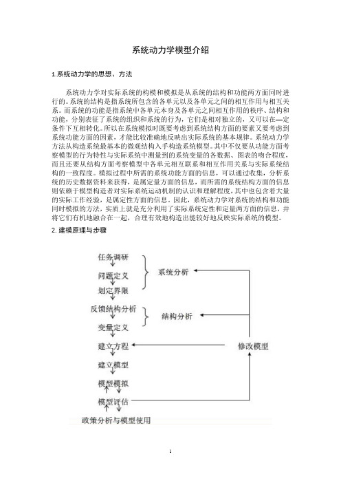
2.建模原理与步骤(1)建模原理用系统动力学方法进行建模最根本的指导思想就是系统动力学的系统观和方法论。

系统动力学认为系统具有整体性、相关性、等级性和相似性。

系统内部的反馈结构和机制决定了系统的行为特性，任何复杂的大系统都可以由多个系统最基本的信息反馈回路按某种方式联结而成。

系统动力学模型的系统目标就是针对实际应用情况，从变化和发展的角度去解决系统问题。

系统动力学构模和模拟的一个最主要的特点，就是实现结构和功能的双模拟，因此系统分解与系统综合原则的正确贯彻必须贯穿于系统构模、模拟与测试的整个过程中。

与其它模型一样，系统动力学模型也只是实际系统某些本质特征的简化和代表，而不是原原本本地翻译或复制。

系统动力学模拟软件Vensim使用指南严广乐张志刚（上海理工大学管理学院）在目前系统动力学专用的计算机模拟语言软件中，V ensim是界面非常友好的一种模拟工具，它的功能非常强大，可以运行方程数目达数千的大型模型，因此被人们广泛使用，如美国的国家模型等。

一、Vensim软件简介Vensim是美国Ventana Systems公司推出的在Windows操作平台下运行的系统动力学专用软件包，其版本在不断升级，目前最新的版本为V5.0c。

Vensim PLE是Ventana Systems公司提供的个人学习版，可到公司的网站上免费下载试用。

1.1 Vensim软件的主要特点Vensim是一款可视化的模型工具，使用该软件可以对动力学系统模型进行概念化、模拟、分析和优化。

Vensim PLE和PLE Plus是为简化系统动力学的学习而设计的Vensim的标准版本。

Vensim PLE提供了一个非常简单易用的基于因果关系链、状态变量和流图的建模方式。

Vensim用箭头来连接变量，系统变量之间的关系作为因果连接而得到确立，方程编辑器可以帮助方便地建立完整的模拟模型。

通过建立过程、检查因果关系、使用变量以及包含变量的反馈回路，可以分析模型。

当建立起一个可模拟的模型，Vensim可以从全局来研究模型的行为。

Vensim PLE适合于建立规模较小的系统动力学模型，而Vensim PLE Plus功能则更加强大，支持多视图，适合于大型的模型模拟。

Vensim提供了对所建模型的多种分析方法。

Vensim可以对模型进行结构分析和数据集分析，结构分析包括原因数分析、结果树分析和反馈回列表分析，数据集分析包括变量随时间变化的数据值及曲线图分析。

此外，Vensim还可以实现对模型的真实性检验，以判断模型的合理性，从而相应调整模型的参数或结构。

1.2 Vensim PLE的用户界面Vensim PLE的用户界面是标准的Windows应用程序界面。

vensim操作⼿册（系统动⼒学）Formulating Models of Simple SystemsusingVensim PLEversion 3.0BProfessor Nelson RepenningSystem Dynamics GroupMIT Sloan School of ManagementCambridge, MA O2142Edited by Laura Black, Farzana S. Mohamed, and students in the System Dynamics in EducationProject, April 1998.Copyright ? 1998 by the Massachusetts Institute of Technology.I. Introduction and Getting StartedThe purpose of this tutorial is to help you develop some familiarity with building and analyzing system dynamics models using the Vensim PLE software. In order to become familiar with Vensim PLE, you are going to build a simple model of the federal deficit.To begin you need to get Vensim PLE ready for modeling. This tutorial makes use of the Macintosh version on Vensim PLE; the IBM-Compatible version should work similarly, but some of the screens may look different. When you first open Vensim PLE on your computer, the screen should look like this:To start working on a new model go to the File menu and select New Model. Vensim PLE will return the following dialog box:To begin your effort you must choose the time horizon of your model (when your simulation will start and finish), the appropriate time step (how accurately you wish to simulate your model), and the units of time. Start your model of the deficit in 1988 (enter 1988 in the INITIAL TIME box) and simulate it through the year 2010. Select a time step of 0.25 years. Finally, change the units of time from Month to Year. Your dialog box should now look like this:Click on OK or hit return. To give your model a name, choose the Save As... command from the File menu and enter the desired name in the text field and click on OK. (Vensim PLE should automatically supply the .mdl extension. If you are working with a different version of Vensim and see a Show all of type option on the right side of the dialog box, make sure that the .mdl Fmt Models extension is selected. This allows Vensim PLE to save the model in a format that can be used by both Macintosh and IBM-compatible computers.)?Vensim saves every simulation run and custom graph you produce as a separate file. It supplies a .vdf extension for simulation runs. These files cannot be opened from outside the Vensim application; they can be opened from inside Vensim through the Datasets / Simulate Model... and Control / Custom Graphs dialog boxes.Your screen should now look like this:You are ready to start building your model.II. Developing the Stock, Flow, and Feedback StructureThe Vensim PLE software is designed using the metaphor of a “work bench.” The large blank area in the middle of the screen is your work area, where you actually develop and analyze your model. The different buttons on the border of the work area represent the different “tools”available as you work on your model. The upper toolbar consists of the Title Bar, a Menu, a Main Toolbar, and Sketch Tools. The Main Toolbar comprises two sets of tools: file operation tools that control standard file functions—opening, closing and saving files, printing, cutting, copying, and pasting—as well as simulation and graphing tools that will allow you to set up and run simulations, and set up display graphs. The sketch tools allow you to build in model components. The tools on the Status Bar (the bottom of the window) allow you to change the formatting of the diagram. The Analysis Tools on the left on the window are tools that you will use to analyze your model to understand its behavior. You will become familiar with many of these tools as you build the deficit model.To begin, add a stock representing the outstanding federal debt to your model. Click on theYou have just created the first variable in your model, the stock of money that constitutes the federal debt.Now, add the inflow to the stock of Debt. Click on theNote: Thetool and then click on the flow valve. This action will remove the flow from the model and let you start over again.You have now created the flow, Net Federal Deficit, which increases the stock of Debt.At this point you may you wish to change the name of the stock variable from Debt to FederalDebt. Click on theNow you need to create the variables needed to determine the Net Federal Deficit. Assume the Net Federal Deficit is determined by two variables, Government Revenues and TotalGovernment Expenses. Click on thebutton to select the causal arrow tool. Now, click and release on the variable Government Revenue and then click and release again on Net Federal Deficit. Do the same for Total Government Expenses. Make sure your causal arrows actually end on the words Net Federal Deficit. They should not be attached to the cloud, the stock, or directly to the valve.You can delete arrows using theClicking on theNow, you may want to update your diagram by labeling the arrows to show that Government Revenue and Total Government Expense affect the Net Federal Deficit in different ways. Specifically, an increase in revenue causes the deficit to decrease, while an increase in expenses causes the deficit to increase. To do this, first click on thebutton on the bottom horizontal toolbar. You then see a pop-up menu that looks like this:Click and release on the desired label, and it will show up in the diagram. Label your two causal arrows so your diagram looks like this:Now, using the same steps discussed above, complete the stock, flow and feedback so your diagram looks like this:You may want to slide the handle of each arrow close to its arrowhead, so each label is clearly associated with its causal arrow.Finally, you may wish to label the positive feedback loop you have just created. Click on theClick on the Loop Clkwse button in the Shape box; click on Center in the Text Position box; and type R, for reinforcing, in the Comment box. You may also type + or P to denote a positive feedback, also known as a reinforcing, loop. Your screen should now look like this:Click on the OK button or hit return. Your screen should now appear as:III. Specifying Equations for Your ModelNow that you have developed a complete stock, flow, and feedback representation of the deficit, you need to write equations for each of the variables. Equation formulation is a critical step in the process of model building and is a key part of the process of developing a rigorous understanding of the problem at hand.To begin writing equations, click on theA highlighted variable indicates that the equation for that variable is incomplete.Variables in system dynamics models are classified as either exogenous or endogenous. Exogenous variables are those that are not part of a feedback loop, while endogenous variables are members of at least one feedback loop. Your deficit model has three exogenous variables—Government Revenue, Other Government Expenses, and the Interest Rate—and four endogenous variables—Interest Payments, Total Government Expense, Net Federal Deficit, and the Federal Debt.Start by writing the equations for the exogenous variables. To begin, click on the highlighted variable Government Revenue. You then see the following dialog box:Good modeling practice requires that each equation in a model have three elements: the equation itself, specified units of measure, and complete documentation. You enter the equation in the box to the right of the = sign. You enter the unit of measure in the text field to the right of the word Units. Equation documentation or “comment” is entered in the box to the right of the word Comment.To write an equation for Government Revenue, click in the box to the right of the = sign. Assume that government revenue is constant, so that all you need to do is enter the appropriate number for government revenue. In 1988, government revenue was about 900 billion dollars annually, so type 900000000000 in the box. Alternatively, you can write 9e11, which is Vensim PLE shorthand for 9 * 1011.Now, fill in the units. Revenue is a flow variable, so the appropriate unit of measure for this equation is dollars/time unit. Because you already chose to run the model in time steps of 1 year, the appropriate unit is dollars/year. Type dollars/year in the units field. (The next time you specify the units for a variable in this model, dollars/year will appear in the units pull-down menu. You can click on the arrowhead to the right of the units field to see units already specified for other variables in the model, and then use the mouse to select the units from that list when appropriate.) Finally, provide a description of this equation in the comment field. A good comment will be brief, but it will also give the reader the logic behind the equation as well as state the key assumptions. For example, one might write for this equation:Government revenues are assumed to be constant and equal to 900 billiondollars annually based on the actual value in 1988.Your dialog box should now look like this:Click on OK or hit return and your diagram will look like this:Government Revenue is no longer highlighted because you have just specified its equation.Following the process above, write equations for the two other exogenous variables, Interest Rate and Other Government Expenses. Use the following information:Government expenses, excluding interest on the debt, were approximately 900 billion dollars in 1988.The interest rate paid on the national debt in 1988 was around 7%/year.Now that the equations for the exogenous variables are formulated, turn your attention to the endogenous variables. Writing equations for the stocks and the flows is a little different, so let’s do an example of each. First we formulate the equation for the stock, Federal Debt.Again, click on theThe following dialog box will be displayed:Unlike flows and constants, a stock requires that an additional element be specified in its formulation; after you specify the equation, you need to select an initial or starting value.You enter the equation for the stock in the box to the right of the word Integ. Integ stands for “integrate” and simply means that the stock at any moment in time is equal to the sum of all the inflows minus the sum of all the outflows plus the initial value. When you created the stock, flow, and feedback diagram, you connected the flow Net Federal Deficit to the stock Federal Debt. Vensim PLE captures this stock-flow dependency by providing a list of the required Variables to the stock Federal Debt on the right side of the equation dialog box. (The variable we are formulating, Federal Debt, itself also appears in the Variables box, but we focus on the input Net Federal Deficit. In general, you will never want to have the same variable onboth the left and right sides of an equation.)Because the model diagram shows the flow Net Federal Deficit feeding into the stock Federal Debt, Vensim has anticipated that the flow is an input to the stock equation and has placed the Net Federal Deficit variable name in the box to the right of Integ. If this is not the case in your version of Vensim PLE, then simply click in the box to the right of the Integ and then click on the variable Net Federal Deficit in the Variables box to write the equation for the change in Federal Debt. (Note:If Net Federal Deficit is not in the Variables box, then your model diagram is incorrect and needs to be changed—make sure the flow is attached to the stock).The Integ box should now look like this:Below the Integ box is the Initial Value box. Here you enter the initial condition or starting point for the stock. In 1988, the outstanding federal debt was approximately 2.5 trillion dollars, so enter 2500000000000 in the initial value box (alternatively you can write 2.5e12, which is Vensim PLE shorthand for 2.5 x 1012). The Initial Value box should look like this:Now the equation specification for the Federal Debt stock is complete. Your equation indicates that the federal debt is simply the accumulation of the Net Federal Deficit since 1988 added to the initial value.You still need to specify the unit of measure and document your equation in the comment field. The units should be fairly straightforward. The Federal Debt is a stock and its units are dollars. Useful comments briefly explain the structure of the equation and highlight the key assumptions made. A sample comment for Federal Debt is:The Federal Debt is the accumulation of the Net Federal Deficit plus theinitial value of the debt. The initial value is set to 2.5 trillion dollars,which was the approximate outstanding federal debt in 1988—the startingpoint for this simulation.Your dialog box should now look like this:。

第1章概述1.1.系统动力学简介1956年，Jay W.Forrester 放弃了其在电机控制领域的研究，转而将反馈控制的基本原则用于社会经济学系统。

1961年，他在MIT工业管理学院研究公司管理问题，出版了其专著Industrial Dynomics, 这标志着这一学科的创立。

在过去的40年中，系统动力学有了长足的发展。

系统动力学的理论、思想方法和工具，对于分析社会经济中许多复杂动态问题非常有效。

另一方面，系统动力学的分析方法、建模方法、模拟方法和模拟工具比较规范，易于学习和应用。

1、事件－行为－结构在日常生活中，我们往往是从事件开始认识事物的。

例如股市暴涨暴跌，流行病发生，战争爆发等等。

事件一般是在固定的时间点上出现的。

我们要正确的认识事件，须要联系相关事件，并从它们的发展过程中去观察。

也即，要考察事件所在的行为模式。

行为模式是系统的外在表现，可表现为一系列的相关事件随事件的演变过程，是多个关联事件表现出的过去现在和未来。

例如，我们看到的经济的缓慢增长，利率的变化，失业率的波动等。

行为摸式是由系统的内部结构决定的。

结构是产生行为模式的物质的、能量的、信息的内在关系。

系统的结构决定其行为模式，而事件是行为模式的重要片段。

利用系统动力学分析问题，要由事件出发，分析系统的结构与行为模式的关系，以采取成功的政策和策略，调整系统结构，干预和控制系统，改善系统的行为模式，大大避免坏的事件的发生。

2、系统动力学处理问题的过程●提出问题：明确建立模型的目的。

即要明确要研究和解决什么问题。

●参考行为模式分析：分析系统的事件，及实际存在的行为模式，提出设想和期望的系统行为模式。

作为改善和调整系统结构的目标。

●提出假设建立模型：由行为模式，提出系统的结构假设。

由假设出发，设计系统的因果关系图，流图，并列出方程，定义参数。

从而将一系列的系统动力学假设，表示成了清晰的数学关系集合。

●模型模拟：调整参数，运行模型，产生行为模式。

“捕食者-被捕食者”——基于Vensim的模型模拟14307130034光电信息科学与工程毛臻岑-目录-一、模型背景 (3)二、建模过程 (4)2.1新建model (4)2.2创建变量、设置方程 (4)2.3绘制因果图流图 (6)三、运行和调试模型： (6)3.1以原始值运行模拟 (7)3.2调整参数，出现平衡 (14)引用及参考： (21)一、模型背景本文参考捕食者-被捕食者模型（Predator-Prey Model），参考《社会系统动力学》第58页所示流图。

二、建模过程2.1新建model开启Vensim 6.4b PLE新建model，参数设置如下：2.2创建变量、设置方程2.3绘制因果图流图三、运行和调试模型：3.1以原始值运行模拟prey：predator：Time(Month)predator Runs:predator 0Current10113217322428535644755869987 10109 111373.2调整参数，出现平衡设置predator死亡速率为1/16，则两个种群的数量基本上达到平衡：prey：Time(Month)prey Runs:prey 0Current1000 11300 21620 31878 41878 51878 61878 71878 81878 91878 101878 111878predator：引用及参考：1.李旭著：社会系统动力学：政策研究的原理、方法和应用[M].上海：复旦大学出版社，ISBN：978-7-309-06360-82.朱老师的ppt。