A Survey on Smoothed Particle Hydrodynamics (SPH)

a r X i v :p h y s i c s /9809020v 1 [p h y s i c s .a t o m -p h ] 15 S e p 1998MuoniumKlaus P.Jungmann Physikalisches Institut,Universit¨a t Heidelberg Philosophenweg 12,D-69129Heidelberg,Germany Abstract.The energy levels of the muonium (µ+e −)atom,which consists of two ”point-like”leptonic particles,can be calculated to very high accuracy in the framework of bound state Quantum Electrodynamics (QED),since there are no complications due to internal nuclear structure and size which is the case for all atoms and ions of natural isotopes including atomic hydrogen.The ground state hyperfine splitting and the 1s-2s energy interval can provide both tests of QED theory and determinations of fundamental constants like the muon mass m µand the fine structure constant α.The excellent understanding of the electromagnetic binding in the muonium atom allows in particular testing fundamental physical laws like lepton number conservation in searches for muonium to antimuonium conversion and probing the nature of the muon as a heavy leptonic object.I INTRODUCTION Atomic hydrogen has played an important role in the history of modern physics.The successful description of the spectral lines of the hydrogen atom by the Schr¨o dinger equation [1]and especially by the Dirac equation [2]had a large impact on the development of quantum mechanics.Precision measurements of the ground state hyperfine structure splitting by Nafe,Nelson and Rabi [3,4]in the late 1940’s were important contributions to the identification of the magnetic anomaly of the electron.Together with the observation of the “classical”22S 1/2−22P 1/2Lamb shift by Lamb and Retherford [5]they pushed the development of the modern theory of Quantum Electrodynamics(QED).Today the anomalous magnetic moment of the electron,which is defined as a e =(g e −2)/2,where g e is the electron g-factor,and the ground state hy-perfine structure splitting ∆νH HF S of atomic hydrogen are among the most wellknown quantities in physics.Experiments in Penning traps with single elec-trons [6]have determined a e =1159652188.4(4.3)·10−12to 3.7ppb.QED cal-culations have reached such a precision that the fine structure constant αcan be extracted to 3.8ppb [7].Hydrogen hyperfine structure measurements yield ∆νH HF S =1420.4057517667(9)MHz (0.006ppb)[8,9]and hydrogen masers even have a large potential as frequency standards.However,the theoretical descriptionof the hyperfine splitting is limited to the ppm level by the fact that the proton’s internal structure is not known well enough for calculations of nearly similar accu-racy[10,11].Neither can experiments supply the necessary data on the mean square charge radius and the polarizability,for example from electron scattering,nor is any theory,for example low energy quantum chromodynamics(QCD),in a posi-tion to yield the protons internal charge structure and the dynamical behavior of its charge carrying constituents.The situation is similar for the2S1/2-2P1/2Lambshift in hydrogen,where atomic interferometer experimentsfind∆νH2S1/2−2P1/2=1057.8514(19)MHz[12](1.8ppm)and where the knowledge of the proton’s mean square charge radius limits any calculations to the10ppm level of precision[10,11]. The1s-2s level separation in atomic hydrogen has reached a fascinating accuracy for optical spectroscopy and one can expect even further significant improvements. The Rydberg constant has been extracted to R∞=10973731.568639(91)m−1 [13,14]by comparing this transition with others in hydrogen and is now the best known fundamental constant.However,the knowledge of the mean square charge radius limits comparison between experiment and theory.Detailed reviews on this topic were given by[15,16]on this conference.TABLE1.The ground state hyperfine structure splitting∆νHF S and the1s-2s level separation ∆ν1S−2S of hydrogen and some exotic hydrogen-like systems offer narrow transitions for studying the interactions in Coulomb bound two-body systems.In the exotic systems the linewidth has a fundamental lower limit given by thefinite lifetime of the systems,because of annihilation,as in the case of positronium,or because of weak muon or pion decay.The very high quality factors (transition frequency divided by the natural linewidth∆ν/δν)in hydrogen and other systems with hadronic nuclei can hardly be utilized to test the theory because of the insufficiently known charge distribution and dynamics of the charge carrying constituents within the hadrons.Positronium Hydrogen Pioniume+e−pe−π+e−∆ν1S−2S2455.62468.5 4.59×105 [THz]δν1S−2S.145.145.176 [MHz]∆νHF S1.7×102 3.2×1024--†Only the1S-2S splitting in the triplet system of positronium is considered in this table. In addition to the information obtainable from the natural isotopes hydrogen (pe−),deuterium(de−)and tritium(te−)or hydrogen-like ions of natural elements((Z A Xe−)(Z−1)+),exotic hydrogen-like atoms can provide further information about the interactions between the bound particles and the nature of these objects them-selves[17].Such systems can be formed by replacing the electron in a natural atom by an exotic particle(e.g.µ−,π−,K−,In purely hadronic systems like pionic hydrogen(pπ−)and antiprotonic hydro-gen[32],protonium(pK0system[54],where the relative mass difference is≤4·10−18.Precision experiments on muonium offer a unique opportunity to investigate bound state QED without complications arising from nuclear structure and to test the behavior of the muon as a heavy leptonic particle and hence the electron-muon(-tau)universality,which is fundamentally assumed in QED theory.Of particular interest is the ground state hyperfine structure splitting,where experiment[55]and theory[10,11]agree at300ppb which is at a higher level of precision than in thecase of atomic hydrogen.An accurate value for the fine structure constant αcan be extracted to 140ppb.The Zeeman effect of the ground state hyperfine sublevels yields the most precise value for muon the magnetic moment µµwith an accuracyof 360ppb.Signals from the ”classical”22S 1/2-22P 1/2Lamb shift in muonium have been observed [56,78].However,with 1.4%precision they are not yet in a region where they can be confronted with theory.The sensitivity to QED corrections is highest for the 1S-2S interval in muonium due to the approximate 1/n 3scaling of the Lamb pared to hydrogen,the radiative recoil and the relativistic recoil effects are larger by a factor of m p /m µ≈8.9,where m p is the proton mass and m µthe muon mass.A hydrogen-muonium isotope shift measurement in this transition as well as a technically only slightly more difficult measurement of the 1s-2s transition frequency in muonium can lead to a new and accurate figure for the muon mass m µ.The transition has recently been excited successfully in two independent experiments [57–60].2S 21/21S 21/2 F = 1F = 0F = 1F = 0F = 1558 MHz λ = 244 nmλ = 244 nm 22P 3/22P 1/22 F = 21047 MHz F = 1F = 074 MHz 187 MHz 9875 MHz ∆ν = 4463 MHz HFS ∆ν = 2455 THz1s2s FIGURE 1.Energy levels of muonium for principal quantum numbers n=1and n=2.The indicated gross,fine and hyperfine structure transistions were studied yet.The most accurate measurements are the ones involving the n=1ground state in which the atoms can be produced efficiently.The spectroscopic experiments in muonium are closely inter-related with the determination of the muon’s magnetic anomaly a µthrough the relation µµ=(1+a µ)eh ¯/(2m µc ).The results from all experiments establish a self consis-tency requirement for QED and electroweak theory and the set of fundamental constants involved.The constantsα,mµ,µµare the most stringently tested impor-tant parameters.The only necessary external input are the hadronic correctionsto aµwhich can be obtained from a measurement of the ratio of cross sections(e+e−→µ+µ−)/(e+e−→hadrons).Although,in principle,the system could provide the relevant electroweak constants,the Fermi coupling constant G F andsin2θW,the use of more accurate values from independent measurements may bechosen for higher sensitivity to new physics.As a matter of fact,an improve-ment upon the present knowledge of the muon mass at the0.35ppm level is veryimportant for the success of a new measurement of the muon magnetic anomaly presently under way at the Brookhaven National Laboratory in Upton,New York. The relevance of the experiment,which aims for0.35ppm accuracy,arises from its sensitivity to contributions from physics beyond the standard model and the clean test it promises for the renormalizability of electroweak interaction[61,62].II GROUND STATE HYPERFINE INTER V ALThe ground state hyperfine splitting allows the most sensitive tests of QED for the muon-electron interaction.An unambiguous and very precise atomic physics value for thefine structure constantαcan be derived from∆νHF S.The experimental precision for∆νHF S has reached the level of0.036ppm or160Hz which is just a factor of two above the estimated contribution of-65Hz(15ppb)from the weak interaction arising from an axial vector–axial vector coupling via Z-boson exchange [63,64].The sign of the weak effect is in muonium is opposite to the one for hydrogen,because the positive muon is an antiparticle and the proton is a particle. (Therefore the muonium atom may be viewed as a system which is neither pure matter nor antimatter.)With increased experimental accuracy muonium can be thefirst atom where a shift in atomic energy levels due to the weak interaction will be observed.A contribution of250Hz(56ppb)due to strong interaction arises from hadronic vacuum polarization.The theoretical calculations for∆νHF S can be improved to the necessary precision[65].The calculations themselves are at present accurate to about50ppb.However,there is a300ppb uncertainty arising from massµµof the positive muon.All precision experiments to date have been carried out with muonium formed by charge exchange after stoppingµ+in a suitable gas[48].The experimental part of such an effort[73]has been completed at the Los Alamos Meson Physics Facility(LAMPF)and the recorded data are presently being analyzed.The exper-iment used a Kr gas target at typically atmospheric pressures and a homogeneous magneticfield of about1.7Tesla.Microwave transitions between Zeeman levels which involve a muon spinflip can be detected through a change in the spatial distribution of positrons from muon decays,since due to parity violation in the decay process the positve muons decay with the positrons preferentially emitted inTABLE2.Results extracted from the1982measurement of the muonium ground state hyperfine structure splitting in comparison with some recent theoretical values and rele-vant quantities from independent experiments.∆νHF S(theory)4463302.55(1.33)(0.06)(0.18)kHz(0.30ppm)[66]∆νHF S(theory)4463303.27(1.29)(0.06)(0.59)kHz(0.35ppm)[67]∆νHF S(theory)4463303.04(1.34)(0.04)(0.16)(0.06)kHz(0.30ppm)[69]∆νHF S(theory)4463302.89(1.33)(0.03)(0.00)kHz(0.30ppm)[70]∆νHF S(expt.)4463302.88(0.16)kHz(0.036ppm)[7]α−1(∆νHF S)137.035988(20)(0.15ppm)[7]α−1(electron g-2)137.03599993(52)(0.004ppm)[7]α−1(condensed matter)137.0359979(32)(0.024ppm)[71]µµ/µp(∆νHF S) 3.1833461(11)(0.36ppm)[7]µµ/µp(µSR in lq.bromine) 3.1833441(17)(0.54ppm)[72] muon spin direction.The experiment employed the technique of”old muonium”which allowed to reduce the linewidth of the signals can be reduced below half of the”natural”linewidthδνnat=(π·τµ)−1=145kHz,whereτµis the muon lifetime of2.2µ.For this purpose the basically continuous beam of the LAMPF stopped muon channel was chopped by an electrostatic kicker device into4µs long pulses with14µs separation.Only atoms which were interacting with the microwave field for periods longer than several muon lifetimes were detected[74].The basi-cally statistically limited results improve the knowledge of both zerofield hyperfine splitting and muon magnetic moment by a factor of three[75,76].Thefinal results are discussed in detail in[75].They yield for the zerofield splitting∆νHF S=4463302764(54)Hz(12ppb)(1)which agrees well with the most updated theoretical value[65]∆νtheory=4463302713(520)(34)(<100)Hz(120ppb).(2)For the magnetic moment onefindsµµ/µp=3.18334526(39)(120ppb)(3)which translates into a muon-electron mass ratio ofmµ/m e=206.768270(24)(120ppb).(4)As the hyperfine splitting is proportional to the fourth power of thefine structure constantα,the improvement inαwill be much better and the value is comparable in accuracy with the value ofαdetermined using the Quantum Hall effect.α−1M−HF S=137.0360108(52)(39ppb).(5)Here the value h¯/m e as determined with the help of measurements of the neutron de Broglie wavelength[81]has been benefitially employed to gain higher accuracy2040(νMW - 1897*103) ∈kHz ∉(N M W -o n -N M W -o f f )/N M W -o f f ∈%∉02040(νMW - 2565*103) ∈kHz ∉(N M W -o n -N M W -o f f )/N M W -o f f ∈%∉FIGURE 2.Conventional and ’old’muonium lines.The narrow ’old’lines are also higher.The frequencies ν12and ν34correspond to transitions between (a)the two energetically highest respectively (b)two lowest Zeeman sublevels of the n=1ground state.As a consequence of the Breit-Rabi equation describing the behaviour of the levels in a magnetic field,the sum of these frequencies equals at any fixed field the zero field splitting ∆νand the difference yields for a known field the muon magnetic moment m µ.compared to a previously used determination based on the very well known Rydberg constant which yields α−1M −HF S (traditional )=137.0359986(80)(59ppb ).We can expect a near future small improvement of the value in eq.(5)from ongoing determinations of h ¯/m e through measurements of the photon recoil in Cs atom spectroscopy and a Cs atom mass measurement.The limitation of αfrom muonium HFS,when using eq.(5),arises mainly from to the muon mass.Therefore any better determination of the muon mass,respectively its magnetic moment,e.g.through a precise measurement of the reduced mass shift in the muonium 1s-2s splitting,will result in an improvement of this value of α.It should be noted that already at present the good agreement within two standard deviations between the fine structure constant determined from muonium hyperfine structure and the one from the electron magnetic anomaly is considered the best test of internal consistency of QED,as one case involves bound state QED and the other case QED of free particles.The precision measurements of the muonium hyperfine splitting performed so far,however,suffer from the interaction of the muonium atoms with the foreign gas atoms.With the discovery of polarized thermal muonium emerging from SiO 2powder targets into vacuum [82]measurements of the ∆νHF S are now feasible in vacuum in the absence of a perturbing foreign gas.Corrections for density effects are obsolete.In a preliminary experiment at the Paul Scherrer Institut (PSI)in Villigen,Switzerland,the transitions between the 12S 1/2,F =1and theFIGURE3.Principle of the setup for a measurement of∆νHF S in vacuum.12S1/2,F=0hyperfine levels could be induced in zero magneticfield(see Fig.1). The atoms were formed by electron capture after stopping positive muons close tothe surface of a SiO2powder target.A fraction of these diffused to the surfaceand left the powder at thermal velocities(7.43(2)mm/µs)for the adjacent vacuumregion.A rectangular rf resonator operated in T EM301mode was placed directly above the muonium production target.The atoms entered the cavity with thermalvelocities through a wall opening.The e+from the parity violating muon decayµ+→e++νe+¯νµwere registered in two scintillator telescopes which were mounted close to the side walls of the resonator.The telescope axes have been oriented parallel respectively antiparallel to the spin of the incoming muons which had beenrotated transverse to the muon propagation direction by an ExB separator(Wienfilter)in the muon beam line.At the resonance frequency of4.46329(3)GHz areduction of the muon polarization of16(2)%has been observed as a signal fromthe hyperfine transitions[83].Certainly the method needs a lot of development work in order to improve thesignal strength.However,ultimately one expects higher precision from experiments on muonium in vacuum than from measurements in gases.III LAMB SHIFT IN THE FIRST EXCITED STATEThe classical Lamb shift in the atomic hydrogen atom between the metastable 22S1/2and the22P1/2states is totally QED in nature and seems to be ideal for testing radiative QED corrections.An important contribution arises from the in-ternal proton structure.Its uncertainty limits any theoretical calculation.Today,FIGURE4.First observed muonium∆νHF S signal in vacuum. experiment and theory agree on the10ppm level.The purely leptonic muonium atom is free from nuclear structure problems.In addition,the relativistic reduced mass and recoil contributions are about one order of magnitude larger compared to mb shift measurements at TRIUMF[77]and LAMPF[78,79]have reached the10−2level of precision.TABLE3.n=2Lamb shift in parison between experiment and the-ory.Experiment∆ν22S1/2−22P1/2[MHz]experimental method Ref.been extracted to∆νLS=6988(33)(46)MHz;this the most precise experimental Lamb shift value for muonium available today.From the isotope shifts between the muonium signal and the hydrogen and deuterium1S-2S two-photon resonances we deduce the mass of the positive muon as mµ=105.65880(29)(43)MeV/c2. An alternate interpretation of the result yields the best test of the equality of the absolute value of charge units in thefirst two generations of particles at the10−8 level[60].A new measurement of the1S-2S energy splitting of muonium by Doppler-free two-photon spectroscopy has been performed at the worlds presently brightest pulsed surface muon source which exists at RAL.Increased accuracy is expected compared to a previously obtained value.The series of experiments aims for an improvement of the muon mass.ser system employed in the new muonium1s-2s experiment.The12S1/2(F=1)→22S1/2(F=1)transition was induced by Doppler-free two-photon laser spectroscopy using two counter-propagating laser beams of wavelength λ=244nm.The necessary high power UV laser light was generated by frequency tripling the output of an alexandrite ring laser amplifier in crystals of LBO and BBO.Typically UV light pulses of energy3mJ and80nsec(FWHM)duration were used.The alexandrite laser was seeded with light from a continuous wave Ti:sapphire laser at732nm which was pumped by an Ar ion laser.Fluctuations of the optical phase during the laser pulse were compensated with an electro-optic device in the resonator of the ring amplifier to give a frequency chirping of the laser light of less than about5MHz.The laser frequency was calibrated by frequency modulation saturation spectroscopy of a hyperfine component of the5-13R(26) line in thermally excited iodine vapour.The frequency of the reference line is about700MHz lower than1/6of the muonium transition frequency.The cw light was frequency up-shifted by passing through two acousto-optic modulators (AOM’s).The muonium reference line has been calibrated preliminarily to3.4MHz at the Institute of Laser Physics in Novosibirsk.An independent calibration at theNational Physics Laboratory(NPL)at Teddington,UK,was performed to140kHz (0.35ppb).FIGURE6.The1S1/2(F=1)→2S1/2(F=1)transition signal in muonium,not corrected for systematic shifts due to frequency chirping and ac Stark effect.The1S-2S transition was detected by the photoionization of the2S state by a third photon from the same laserfield.The slow muon set free in the ionization process is accelerated to2keV and guided through a momentum and energy selec-tive path onto a microchannel plate particle detector(MCP).Background due to scattered photons and other ionized particles can be reduced to less than1event in5hours by shielding and by requiring that the MCP count falls into a100nsec wide window centered at the expected time offlight for muons and by additionally requiring the observation of the energetic positrons from the muon decay.On res-onance an event rate of9per hour was observed.The number of MCP events as a function of the laser frequency is displayed in Fig.6.The line shape distortions due to frequency chirping were investigated theoreti-cally using density matrix formalism tofind numerically the frequency dependence of the signal for the time dependent laser intensity and the time dependent phase of the laserfield which were both measured for every individual laser shot using fast digitzed amplidude and optical heterodyne signals[84,85].The model was verified experimentally at the ppb level by observing resonances in deuterium and hydro-gen.A careful analysis of the recorded muonium data is in progress and promisses for thefirst succesful run with the new all solid state laser system an accuracy of order10MHz which is significantly better than the previous result.The measure-ments are still limited by properties of the laser system,in particular by the chirp effect,rather than by statistics.It can be expected that future experiments will reach well below1MHz in accu-racy promising an improved muon mass value.The theoretical value at present is basically limited by the knowledge of recoil terms at the0.6MHz level.Here some improvement of calculations will become important for the next round of experi-ments.V MUONIUM TO ANTIMUONIUM CONVERSIONA spontaneous conversion of muonium(M=µ+e−)into antimuonium(K0oscillations[86].Since lepton number is a solely empirical law and no underlying symmetry could yet be revealed,it can be reliably applied only to the level at which it has been tested.The M-M ,where GMFIGURE8.Topview of the MACS(Muonium-Antimuo-nium-Conversion-Spectrometer)appara-tus at PSI to searchfor M−M≤8.2·10−11/S B(90% C.L.)was found,where S B accounts for the interaction type dependent suppres-sion of the conversion in the magneticfield of the detector due to the removal of degeneracy between corresponding levels in M andM≤3.0·10−3G F(90%C.L.)with G F the weak interaction Fermi constant. This new result,which exceeds bounds from previous experiments[89,107]by a factor of2500and the one from an early stage of the experiment[88]by35,has some impact on speculative models.A certain Z8model is ruled out with more than4generations of particles where masses could be generated radiatively with heavy lepton seeding[108].A new lower limit of m X±±≥ 2.6TeV/c2∗g3l(95%C.L.)on the masses of flavour diagonal bileptonic gauge bosons in GUT models is extracted which lies well beyond the value derived from direct searches,measurements of the muon magnetic anomaly or high energy Bhabha scattering[104,98].Here g3l is of order 1and depends on the details of the underlying symmetry.For331models this translates into m X±±≥850GeV/c2which excludes their minimal Higgs version in which an upper bound of600GeV/c2has been extracted from an analysis ofelectroweak parameters[109,110].The331models may still be viable in someextended form involving a Higgs octet[111].In the framework of R-parity violating supersymmetry[103,95]the bound on the coupling parameters could be lowered by a factor of15to|λ132λ∗231|≤3∗10−4for assumed superpartner masses of 100GeV/c2.Further the achieved level of sensitivity allows to narrow slightly theinterval of allowed heavy muon neutrino masses in minimal left-right symmetry[101](where a lower bound on GMM conversion is allowed,the process is intimately connected to the lepton family number violating muon decay µ+→e++νµ+√M interaction is below1.5Hz/M experiment could take particularly advantage of high intense pulsed beams.In contrast to other leptonflavour violating muon decays,the con-version through its nature as particle-antiparticle oscillation,has a time evolution in which the probability forfindingvarious places.In the intermediate future the Japanese Hadron Facility(JHF)or a possible European Spallation Source(ESS)are important options.Also the dis-cussed Oak Ridge neutron spallation source could in principle accommodate intense muon beams.The most promising facility would be,however,a muon collider[114], the front end of which could provide muon rates5-6orders of magnitude higher than present beams(see Table4).TABLE4.Muonfluxes of some existing and future facilities,Rutherford Appleton Laboratory (RAL),Japanese Hadron Facility(JHF),European Spallation Source(ESS),Muon collider(MC).RAL(µ+)PSI(µ+)PSI(µ−)JHF(µ+)†ESS(µ+)MC(µ+,µ−)3×1063×1081×1084.5×1074.5×1077.5×1013 Momentum bite10101010105-10 Spot size1.2×2.03.3×2.0 3.3×2.0 1.5×2.0 1.5×2.0few×few Pulse structure50Hz continuous continuous50Hz50Hz15Hzmb and R.C.Retherford,Phys.Rev.79,549(1950),and Phys.Rev.71,241(1947)6.R.S.Van Dyck,Jr.,in:Quantum Electrodynamics,T.Kinoshita(ed.),World Sci-entific,Singapore,p.322(1990)7.T.Kinoshita,IEEE.Trans.Instr.Meas.46,108(1997)8.L.Essen,R.W.Donaldson,M.J.Bangham,and E.G.Hope,Nature229110(1971)9.H.Hellwig,R.F.C.Vessot,M.W.Levine,P.Zitzewitz,D.W.Allen,and D.J.Glaze,IEEE Trans.Instrum.IM-19,200(1970)10.J.R.Sapirstein and D.R.Yennie,in:Quantum Electrodynamics,T.Kinoshita(ed.),World Scientific,Singapore,p.560(1990)11.D.R.Yennie,Z.Phys.C56,S13(1992)12.V.G.Palchikov,Y.L.Sokolov,and V.P.Yakovlev,Metrologia21,99(1985)13.B.de Beauvoir,F.Nez,L.Julien,B.Cagnac,F.Biraben,D.Touahri,L.Hilico,O.Acef,A.Clairon,and J.J.Zondy,Phys.Rev.Lett.78,440(1997).14.Th.Udem,A.Huber,B.Gross,J.Reichert,M.Prevedelli,M.Weitz,and T.W.Hnsch,Phys.Rev.Lett.79,2646(1997);see also:A.Huber,Th.Udem,B.Gross,J.Reichert, M.Kourogi,K.Pachucki,M.Weitz,and T.W.Hnsch,Phys.Rev.Lett.80,468(1998).15.T.W.H¨a nsch,this conference;see also: e.g.Th.Udem, A.Huber, B.Gross,J.Reichert,M.Prevedelli,M.Weitz,and T.W.Hnsch,Phys.Rev.Lett.,79,2646 (1997),B.de Beauvoir,F.Nez,L.Julien,B.Cagnac,F.Biraben,D.Touahri,L.Hilico, O.Acef,A.Clairon und J.J.Zondy,Phys.Rev.Lett.78,440(1997),16.K.Pachucki,this conference17.K.Jungmann,in:Atomic Physics14(New York:AIP Press),D.Wineland et al.(ed.),p.102(1994)18.R.Coombes,R.Flexer,A.Hall,R.Kennelly,J.Kirkby,R.Piccioni,D.Porat,M.Schwartz,R.Spitzer,J.Toraskar,S.Wiesner,B.Budick,and J.W.Kast,in: Atomic Physics5(R.Marrus,M.Prior,and H.Shugart,eds.),Plenum,New York p.95(1977)19.L.Schaller,Z.Phys.C56,S48(1992)20.R.Rosenfelder,in:Muonic Atoms and Molecules,L.Schaller and C.Petitjean(eds.)Birkh¨a user,Basel,p.95(1992)21.K.Jungmann,Z.Phys.C56,S59(1992)22.D.Baklalov,otti,C.Rizzo,A.Vacchi,and E.Zavattini,Phys.Lett.A172277(1993)23.P.A.Souder,T.W.Crane,V.W.Hughes,D.C.Lu,H.Orth,H.W.Reist,M.H.Yam,G.zu Putlitz,Phys.Rev.A22,33(1980)24.H.Orth,K.P.Arnold,P.O.Egan,M.Gladisch,W.Jacobs,J.Vetter,W.Wahl,M.Wiegand,G.zu Putlitz,V.W.Hughes,Phys.Rev.Lett.45,1483(1980)25.C.J.Gardener,A.Badertscher,W.Beer,P.R.Bolton,P.O.Egan,M.Gladisch,M.Greene,V.W.Hughes,D.C.Lu,F.G.Mariam,P.A.Souder,H.Orth,J.Vetter,G.zu Putlitz,Phys.Rev.Lett48,1168(1982)26.G.Carboni,U.Gastaldi,G.Neri,O.Pitzurra,E.Polacco,G.Torelli,A.Bertin,G.Gorini,A.Placci,E.Zavattini,A.Vitale,J.Duclos,and J.Picard,Nuov.Cim.34A,493(1976).27.G.Carboni,G.Gorini,G.Torelli,L.Palffy,F.Palmonari,and E.Zavattini,Nucl.。

第42卷第1期宇航学报Voi.42No.1 2021年1月Journai of Astronautics Januara2021充液航天器变质量液体大幅晃动的SPH分析方法于强，王天舒（清华大学航天航空学院，北京100084）摘要：本文基于非惯性系下的光滑粒子流体动力学（SPH）方法,在以虚粒子设置缓冲层的开口边界处理方法基础上，提出一种流出流量可控的出口边界处理方法，能够根据当前时刻航天器的姿态信息和充液比，计算该动力学时间步下变质量液体晃动对航天器产生的作用力和作用力矩,使得航天器系统动力学的闭环仿真成为可能。

最后，通过与计算流体动力学（CFD）商业软件Flow-3d的计算结果进行对比，用不同工况下的算例验证了该变质量液体晃动动力学分析方法的有效性。

关键词：光滑粒子流体动力学（SPH）；变质量液体；大幅晃动；出口边界；晃动作用力及力矩中图分类号：V412.4+2文献标识码：A文章编号：1000-1328（2021）01-0022-09DOI：10.3873/j.gsn.1000-1328.2021.01.003SPH Method for Large-amplitude LiqiU0Sloshing with VariableMast io LiouiO-filleC SpacecraftYU Qiang,WANG Tian-shu(Schoo-of Aerospace Engineemng,Tsinghua University,Beijing100084,China)Abstract:In this paper,based on the non-inertiai smoothed particle hydrodynamics(SPH)which is a Laarangian mesh-less method,a numericai method reaarding outlet boundara conditions is proposed to limit the flux at the outlet boundary,which is an extension of the methods proposed to the treatment of open boundara conditions based on the buffer layers.According to the spacecraft attitude information and linuid-Silled ratio at the current timc,the SPH solver can calculate the sloshing force and moment exerted by variable-mass liqui aaainst the spacecraft during the dynamic timc step.The SPH solver can be embedded in the closed-loop dynamics sigulation of the whole spacecraft.Finlly,in order to verig the validity of the method,the results from the SPH method are compared with those obtained by a commercial computational fluid dynamics(CFD)software,Flow-3d for dgferent sloshing cases.Keywords：Smoothed particle hydrodynamics(SPH)；Variable-mass liquin；Larve-ymplitude sloshing；Outlet boundary；Sloshing force and momento引言一直以来,充液航天器贮箱内液体燃料及氧化剂的晃动作用对于航天器的姿轨控制都有着不可忽视的影响，甚至可能导致任务失败，对液体晃动问题进行准确分析具有重要的意义。

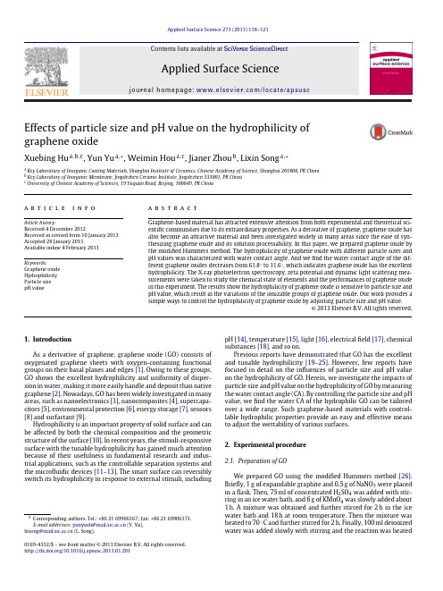
Applied Surface Science 273 (2013) 118–121Contents lists available at SciVerse ScienceDirectApplied SurfaceSciencej o u r n a l h o m e p a g e :w w w.e l s e v i e r.c o m /l o c a t e /a p s u scEffects of particle size and pH value on the hydrophilicity of graphene oxideXuebing Hu a ,b ,c ,Yun Yu a ,∗,Weimin Hou a ,c ,Jianer Zhou b ,Lixin Song a ,∗aKey Laboratory of Inorganic Coating Materials,Shanghai Institute of Ceramics,Chinese Academy of Science,Shanghai 201800,PR China bKey Laboratory of Inorganic Membrane,Jingdezhen Ceramic Institute,Jingdezhen 333001,PR China cUniversity of Chinese Academy of Sciences,19Yuquan Road,Beijing,100049,PR Chinaa r t i c l ei n f oArticle history:Received 4December 2012Received in revised form 10January 2013Accepted 28January 2013Available online 4 February 2013Keywords:Graphene oxide Hydrophilicity Particle size pH valuea b s t r a c tGraphene-based material has attracted extensive attention from both experimental and theoretical sci-entific communities due to its extraordinary properties.As a derivative of graphene,graphene oxide has also become an attractive material and been investigated widely in many areas since the ease of syn-thesizing graphene oxide and its solution processability.In this paper,we prepared graphene oxide by the modified Hummers method.The hydrophilicity of graphene oxide with different particle sizes and pH values was characterized with water contact angle.And we find the water contact angle of the dif-ferent graphene oxides decreases from 61.8◦to 11.6◦,which indicates graphene oxide has the excellent hydrophilicity.The X-ray photoelectron spectroscopy,zeta potential and dynamic light scattering mea-surements were taken to study the chemical state of elements and the performances of graphene oxide in this experiment.The results show the hydrophilicity of graphene oxide is sensitive to particle size and pH value,which result in the variations of the ionizable groups of graphene oxide.Our work provides a simple ways to control the hydrophilicity of graphene oxide by adjusting particle size and pH value.© 2013 Elsevier B.V. All rights reserved.1.IntroductionAs a derivative of graphene,graphene oxide (GO)consists of oxygenated graphene sheets with oxygen-containing functional groups on their basal planes and edges [1].Owing to these groups,GO shows the excellent hydrophilicity and uniformity of disper-sion in water,making it more easily handle and deposit than native graphene [2].Nowadays,GO has been widely investigated in many areas,such as nanoelectronics [3],nanocomposites [4],supercapa-citors [5],environmental protection [6],energy storage [7],sensors [8]and surfactant [9].Hydrophilicity is an important property of solid surface and can be affected by both the chemical composition and the geometric structure of the surface [10].In recent years,the stimuli-responsive surface with the tunable hydrophilicity has gained much attention because of their usefulness in fundamental research and indus-trial applications,such as the controllable separation systems and the microfluidic devices [11–13].The smart surface can reversibly switch its hydrophilicity in response to external stimuli,including∗Corresponding authors.Tel.:+862169906167;fax:+862169906171.E-mail addresses:yunyush@ (Y.Yu),lxsong@ (L.Song).pH [14],temperature [15],light [16],electrical field [17],chemical substances [18],and so on.Previous reports have demonstrated that GO has the excellent and tunable hydrophilicity [19–25].However,few reports have focused in detail on the influences of particle size and pH value on the hydrophilicity of GO.Herein,we investigate the impacts of particle size and pH value on the hydrophilicity of GO by measuring the water contact angle (CA).By controlling the particle size and pH value,we find the water CA of the hydrophilic GO can be tailored over a wide range.Such graphene-based materials with control-lable hydrophilic properties provide an easy and effective means to adjust the wettability of various surfaces.2.Experimental procedure2.1.Preparation of GOWe prepared GO using the modified Hummers method [26].Briefly,1g of expandable graphite and 0.5g of NaNO 3were placed in a flask.Then,75ml of concentrated H 2SO 4was added with stir-ring in an ice water bath,and 6g of KMnO 4was slowly added about 1h.A mixture was obtained and further stirred for 2h in the ice water bath and 18h at room temperature.Then the mixture was heated to 70◦C and further stirred for 2h.Finally,100ml deionized water was added slowly with stirring and the reaction was heated0169-4332/$–see front matter © 2013 Elsevier B.V. All rights reserved./10.1016/j.apsusc.2013.01.201X.Hu et al./Applied Surface Science273 (2013) 118–121119to90◦C and stirred for1h.And the reaction was terminated by addition of100ml deionized water and30ml H2O230wt%aqueous solution.To remove the ions of oxidant and other inorganic impurity, we washed the mixture by repeated vacuumfiltration through a 220nm cellulose acetate membrane.First with5%HCl aqueous solution,and then distilled water until the pH value of the disper-sion was neutral.Then the dispersion was centrifuged(5000rpm for20min),and the supernatant was kept.Finally,the supernatant was diluted with deionized water to a total volume of200ml in a 500mlflask to make a homogeneous GO dispersion for storage. 2.2.Preparation of different particle sizes and pH values of GO aqueous dispersionHomogeneous GO aqueous dispersion was centrifuged (15,000rpm for80min),the supernatant(SGO)was kept and the remnant(RGO)was dispersed in the deionized water by ultrasonication again.And then,the pH value of SGO and RGO dispersion was adjusted by1M HCl or NaOH solution.And SGO and RGO dispersion(about10ml)were then drop coated on clean glass substrates in a clean-room environment and allowed to dry for12h at30◦C.2.3.Characterization and measurement methodsThe particle size distribution of SGO and RGO aqueous dis-persion was characterized by dynamic light scattering(DLS, Brookhaven,USA).And the temperature was kept constant at room temperature.The chemical state of elements in GO was analysed by X-ray photoelectron spectroscopy(XPS,MICROLAB310F,Thermo Scientific,UK),which was equipped with a monochromatic Mg K␣X-ray source.The base pressure of the analyser chamber was less than10−8Torr.The binding energies were calibrated based on the contaminative carbon(C1s=284.6eV).XPS peaks werefitted using Gaussian-like curves and the binding energy values of peaks were given with an accuracy of±0.1eV.The zeta potential of GO was determined as a function of pH using a zeta potential analyser(Zeta-PALS,Brookhaven,USA).The pH value was measured on a model PHS-25pH Meter Instruction(with the precision of0.1).The pH value of SGO and RGO aqueous dispersion was adjusted by1M HCl or NaOH solution.The hydrophilicity of the obtained GO was evaluated with the water contact angle instrument(SL200B,Solon, China)by measuring the contact angle of deionized water droplet. Each deionized water droplet was dropped onto GO surface from 5cm by vibrating the syringe.A5␮L liquid drop was deposited on the surface using a micropipette.Three drops of water were placed at different locations on a horizontal surface,and an average CA value was obtained.All water CA measurements were performed at ambient temperature and saturated humidity.3.Results and discussion3.1.Particle size distributionAs the particle size measurement on DLS was based on the assumption that the particles were spherical,the instrument was unable to give the absolute size of GO.Nevertheless,the measure-ments available provided a quick and effective evaluation of size distribution[27].As shown in Fig.1,the particle size distribution is approximately Gaussian.The particle size distribution of SGO varies from50to175nm,whereas for RGO,it varies from15to80nm.And the nominal effective diameter of particle in RGO and SGO disper-sion is about90and35nm,respectively.The results indicate that SGO has the smaller particle size thanRGO.Fig.1.The particle size distribution of SGO and RGO dispersion.3.2.XPS spectraXPS was also employed to characterize the surface composi-tions of SGO and RGO for its sensitivity to different chemical states of elements.The C1s XPS spectra(solid lines)of SGO and RGO are presented in Fig.2.The spectra are decomposed into threefit-ted peaks(dashed lines)using Gaussian function.A binding energy of285.1eV indicates the existence of C C sp2bonds in GO,while 287.1eV results from C O bonds(epoxy and hydroxyl groups),and 289.2eV gives the evidence of C O bonds(carbonyl group)formed during the oxidation[28].Fig.2.The C1s XPS spectra of(a)SGO and(b)RGO.120X.Hu et al./Applied Surface Science 273 (2013) 118–121Fig.3.Zeta potential of SGO and RGO dispersion under various pH values.Compared with RGO,the C 1s peak with binding energy around 285.1eV of SGO suppresses significantly,suggesting that SGO has a larger number of oxygen-containing functional groups such as C O and C O.3.3.Zeta potentialFig.3shows that the zeta potential of SGO and RGO aqueous dispersion is pH-sensitive.The highest zeta potential value of SGO and RGO dispersion is −47.6mV at pH 10.6and −38.3mV at pH 10.3,respectively.The values are similar to those reported previ-ously [29].The zeta potential provides a measure of the magnitude and sign of the effective surface charge density associated with the double layer around the colloid particle [2].The results in Fig.3show the effective surface charge density increases from RGO to SGO.The results also suggest that the negative charges of GO is a consequence of the ionization of the different groups present [30].And the surface charge density should direct relate to the concen-tration of the ionized groups present at different pH values [31].When the pH is shifted to alkaline,the ionizable groups (carboxylic and/or hydroxyl group)on GO dissociate and GO gains its stronger negative charges.It shows in Fig.4.3.4.Hydrophilicity of GOFrom Fig.5,the water CA of SGO and RGO decreases sharply from 42.3◦to 11.6◦,61.8◦to 33.8◦when the pH value increases from 3.4to 10.5,respectively.Especially,a water CA of 11.6◦was observed for SGO when pH value is 10.5.The smaller water CA suggests that SGO represents the better hydrophilic property.The phenomenon can be explained by the competition between protonation at low pH value and deprotonation at high pH value of the ionizable groups of GO (as showed in Fig.4).These ion-izable groups can accept and donate protons in response totheFig.5.The dependence of water CA on the pH value and particle size of SGO and RGO.Inset:photographs of the water CA of SGO and RGO.environmental change in pH value.As the pH value changes,the degree of ionization of the groups alters dramatically.So,at low pH value,these groups are protonated,rendering the decrease of the surface charge density that causes a larger water CA.As shown in Fig.3,the surface charge density of GO decreases indeed with decreasing pH value.Importantly,from Fig.5,an interesting phenomenon happens on SGO.A smaller water CA is induced in the same pH value,com-pared with RGO.In this situation,the smaller particle size becomes the dominant reason that intensifies the hydrophilicity.It would be explained that the smaller particle size,with the higher edge-to-area ratio (higher surface energy)and more ionizable groups which help interact with water molecules,induces more hydrophilic.XPS (Fig.2)analysis can clarify the change of group distribution of GO with different particle sizes to further prove the above-mentioned description.To determine the effect of particle size on the hydrophilicity,further detailed described by the Young-Dupre equation as follows [21].(1+cos Â)=W(1)where Âis the water contact angle, is the surface free energy of water,W is the work of adhesion (which equals the negative of solid/liquid interfacial energy).The classic model of wetting assumes that the interaction of two surfaces is the summation of all the molecular pair-wise interactions across the interface.Eq.(1)shows the water contact angle (Â)will lower since the work of adhesion (W)increases.So,the hydrophilicity of GO can be understood in terms of how the ionizable groups of GO affect the adsorption energy (solid/liquid interfacial energy)of water molecules on the interface.Consider a water molecule adsorbs on the surface of GO,it interacts with the ionizable groups within the interaction range.The adsorp-tion energy of water on interface changes with the pH valueandFig.4.Schematic illustration shows the surface charge of GO under various pH conditions.The shadowed sections indicate the basal plane of GO.And the circle with subtraction sign depicts the negative charge of GO.X.Hu et al./Applied Surface Science273 (2013) 118–121121particle size of GO.And the adsorption energy(absolute value)increases monotonically with an increasing pH value and decreasing particle size of GO since the higher charge density.From Eq.(1),the water CA should decrease with increasing adsorption energy(if other parameters do not change),thus explaining the predicted water CA results shown in Fig.5.4.ConclusionsA facile approach to modulate the surface wettability of GO with pH value and particle size is demonstrated.The study shows that SGO is better hydrophilic than RGO.The hydrophilicity of GO increases obviously with the higher pH value and smaller particle size.That is the result of the combined effects of the dissociation and number of the ionizable groups of GO,which is confirmed by zeta potential and XPS characterizations.Ourfinding effectively supple-ments the research on the wettability of solid surface based on the pH and size responsive materials,and may expand the application of GO.AcknowledgementsThe authors gratefully acknowledge the support of this research by the National Science Foundation of China(Grant No.51062006). The editor and reviewers are gratefully acknowledged for their good advice.References[1]D.A.Dikin,S.Stankovich,E.J.Zimney,R.D.Piner,G.H.Dommett,G.Evmenenko,S.T.Nguyen,R.S.Ruoff,Nature448(2007)457.[2]B.Konkena,S.Vasudevan,Journal of Physical Chemistry Letters3(2012)867.[3]D.Chen,H.Feng,J.Li,Chemical Reviews112(2012)6027.[4]T.A.Pham,B.C.Choi,K.T.Lim,Y.T.Jeong,Applied Surface Science257(2011)3350.[5]S.D.Perera,R.G.Mariano,N.Nijem,Y.Chabal,J.P.Ferraris,K.J.Balkus,Journalof Power Sources215(2012)1.[6]C.J.Madadrang,H.Y.Kim,G.Gao,N.Wang,J.Zhu,H.Feng,M.Gor-ring,M.L.Kasner,S.Hou,ACS Applied Materials and Interfaces4(2012) 1186.[7]D.Krishnan,F.Kim,J.Luo,R.C.Silva,L.J.Cote,H.D.Jang,J.Huang,Nano Today7(2012)137.[8]Y.Yao,X.Chen,H.Guo,Z.Wu,Applied Surface Science257(2011)7778.[9]L.J.Cote,J.Kim,V.C.Tung,J.Luo,F.Kim,J.Huang,Pure and Applied Chemistry83(2011)95.[10]A.R.Parker,wrence,Nature414(2001)33.[11]N.Nath,A.Chilkoti,Advanced Materials14(2002)1243.[12]A.Kikuchi,T.Okano,Progress in Polymer Science27(2002)1165.[13]N.Verplanck,Y.Coffinier,V.Thomy,R.Boukherroub,Nanoscale Research Let-ters2(2007)577.[14]F.Xia,L.Feng,S.T.Wang,T.L.Sun,W.L.Song,W.H.Jiang,L.Jiang,AdvancedMaterials18(2006)432.[15]T.L.Sun,G.J.Wang,L.Feng,B.Q.Liu,Y.M.Ma,L.Jiang,D.B.Zhu,AngewandteChemie International Edition43(2004)357.[16]R.Rosario,D.Gust,M.Hayes,F.Jahnke,J.Springer,A.A.Garcia,Langmuir18(2002)8062.[17]hann,S.Mitragotri,T.Tran,H.Kaido,J.Sundaram,I.S.Choi,S.Hoffer,G.A.Somorjai,nger,Science299(2003)371.[18]S.Minko,M.Muller,M.Motornov,M.Nitschke,K.Grundke,M.Stamm,Journalof the American Chemical Society125(2003)3896.[19]J.Kim,L.J.Cote,J.X.Huang,Accounts of Chemical Research45(2012)1356.[20]X.Zhang,P.Song,X.Cui,Thin Solid Films520(2012)3539.[21]C.T.Hsieh,W.Y.Chen,Surface and Coatings Technology205(2011)4554.[22]D.R.Dreyer,S.Park,C.W.Bielawski,R.S.Ruoff,Chemical Society Reviews39(2010)228.[23]G.X.Wang, B.Wang,J.S.Park,J.Yang,X.P.Shen,J.Yao,Carbon47(2009)68.[24]J.Y.Kim,L.J.Cote,F.Kim,W.Yuan,K.R.Shull,J.X.Huang,Journal of the AmericanChemical Society132(2010)8180.[25]J.Y.Luo,L.J.Cote,V.C.Tung,A.T.L.Tan,P.E.Goins,J.S.Wu,J.X.Huang,Journal ofthe American Chemical Society132(2010)17667.[26]D.C.Marcano,D.V.Kosynkin,J.M.Berlin,A.Sinitskii,Z.Z.Sun,A.Slesarev,L.B.Alemany,W.Lu,J.M.Tour,ACS Nano4(2010)4806.[27]S.B.Liu,T.Y.H.Zeng,M.Hofmann,E.Burcombe,J.Wei,R.R.Jiang,J.Kong,Y.Chen,ACS Nano5(2011)6971.[28]J.Yang,Y.Zhou,L.Sun,N.Zhao,C.Zang,X.Cheng,Applied Surface Science258(2012)5056.[29]X.Wang,H.Bai,G.Shi,Journal of the American Chemical Society133(2011)6338.[30]D.Li,M.B.Muller,S.Gilje,R.B.Kaner,G.G.Wallace,Nature Nanotechnology3(2008)101.[31]J.A.Yan,L.Xian,M.Chou,Physical Review Letters103(2009)1.。

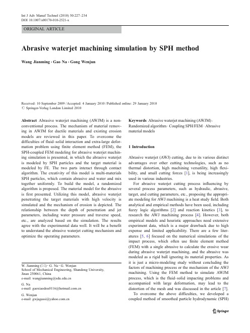
ORIGINAL ARTICLEAbrasive waterjet machining simulation by SPH methodWang Jianming &Gao Na &Gong WenjunReceived:10September 2009/Accepted:4January 2010/Published online:29January 2010#Springer-Verlag London Limited 2010Abstract Abrasive waterjet machining (AWJM)is a non-conventional process.The mechanism of material remov-ing in AWJM for ductile materials and existing erosion models are reviewed in this paper.To overcome the difficulties of fluid –solid interaction and extra-large defor-mation problem using finite element method (FEM),the SPH-coupled FEM modeling for abrasive waterjet machin-ing simulation is presented,in which the abrasive waterjet is modeled by SPH particles and the target material is modeled by FE.The two parts interact through contact algorithm.The creativity of this model is multi-materials SPH particles,which contain abrasive and water and mix together uniformly.To build the model,a randomized algorithm is proposed.The material model for the abrasive is first presented.Utilizing this model,abrasive waterjet penetrating the target materials with high velocity is simulated and the mechanism of erosion is depicted.The relationship between the depth of penetration and jet parameters,including water pressure and traverse speed,etc.,are analyzed based on the simulation.The results agree with the experimental data well.It will be a benefit to understand the abrasive waterjet cutting mechanism and optimize the operating parameters.Keywords Abrasive waterjet machining (AWJM).Randomized algorithm .Coupling SPH/FEM .Abrasive material models1IntroductionAbrasive waterjet (AWJ)cutting,due to its various distinct advantages over other cutting technologies,such as no thermal distortion,high machining versatility,high flexi-bility,and small cutting forces [1],is being increasingly used in various industries.For abrasive waterjet cutting process influencing by several process parameters,such as hydraulic,abrasive,target,and cutting parameters,etc.,proposing the appropri-ate modeling for AWJ machining is a heat study field.Both analytical and empirical methods have been used,including fuzzy logic algorithms [2]and reaction kinetics [3],to research the AWJ machining process [4].However,both empirical models and heuristic approaches need extensive experiment data,which is a major drawback due to high expense and limited applicability.There are a few liter-atures [5,6]focused on the numerical simulations of the impact process,which often use finite element method (FEM)with a single abrasive to calculate the erosive wear during abrasive waterjet machining,and the abrasive was modeled as a rigid ball ignoring its material properties.As it is just a micro-modeling study without concluding the factors of machining process or the mechanism of the AWJ ing the FEM method to simulate AWJM process,which is the fluid –solid impacting problems and accompanied with large deformation,may lead to the distortion of the mesh and was discussed in the article [7].To overcome the above difficulties,we developed a coupled method of smoothed particle hydrodynamic (SPH)W.Jianming (*):G.Na :G.WenjunSchool of Mechanical Engineering,Shandong University,Jinan 250061,Chinae-mail:wangjianming@ G.Nae-mail:gaoxiaodou0116@ G.Wenjune-mail:gwjagassi@Int J Adv Manuf Technol (2010)50:227–234DOI 10.1007/s00170-010-2521-xand FEM.The appeal of SPH for high-velocity AWJ impact is that it is a mesh-free method and belongs to Lagrangian frame,which do not need mesh connectivity so as to allow severe mesh distortions.By SPH method,the continuous material is expressed by a series of particles,which carry some physical quantities such as mass and velocity.This character is regularly adapted for hydrokinetics problems.Johnson and Beissel applied SPH in high-velocity impact-ing problems and got encouraging results [8–10].SPH could overcome the defect of FEM and belongs to Lagrangian frame description,thus,the computation will be more compact and automatic.SPH-coupled FE method-based modeling for abrasive waterjet machining simulation is presented in this paper,in which the abrasive waterjet is modeled by SPH particles and the target material is modeled by finite elements.The two parts interact by contact algorithm of “nodes-to-surface ”in LS-DYNA.The multi-materials SPH particles modeling,in which the abrasives and water mix together uniformly,is first proposed.The randomized algorithm for the actual mass percentage of two materials is used.Based on the explicit program LS-DYNA,the hybrid-code of SPH and FEM is conducted to simulate the machining process,and the simulation result is tested by the experimental data [11].2Basic theory 2.1Basic theory of SPHInstead of a grid,SPH uses a kernel interpolation toapproximate the field variables at any point in a domain.An estimate of the value of a function f (x )at the location x is given in a continuous form by an integral of the product of the function and a kernel (weighting)function W (x −x ′,h )f ðx Þh i ¼ZΩf x 0ðÞW x Àx 0;h ðÞdx 0ð1ÞWhere f ðx Þh i A kernel approximation h Smoothing lengthx ′New independent variable.The kernel function usually has the following properties:Compact support,which means that it is zero every-where but on a finite domain inside the range of the smoothing length 2h :W x Àx 0;h ðÞ¼0forx Àx 0!2hð2ÞNormalized:ZW x Àx 0;h ðÞdx 0¼1ð3ÞThese requirements ensure that the kernel function reduces to the Dirac delta function when h tends to zero:lim h !0W x Àx 0;h ðÞ¼d x Àx 0;h ðÞð4ÞAnd therefore,it follows that:lim h !0f ðx Þh i ¼f ðx Þð5ÞIf the function f (x )is only known at N discrete points,the integral of Eq.1can be approximated by a summation:f ðx Þh i ¼ZΩf x 0ðÞW x Àx 0;h ðÞdx 0%X N j ¼1m j r jf x j ÀÁW x Àx 0j ;h iÀÁð6ÞWhere m j /ρj is the volume associated to the point j orparticle j .Equation 7constitutes the basis of SPH method.The value of a variable at a particle,denoted by subscript i ,is calculated by summing the contributions from a set of neighboring particles (Fig.1),denoted by subscript j and for which the kernel function is not zero:f x i ðÞh i ¼X N j ¼1m j r jf x j ÀÁW x i Àx 0j ;h i ÀÁð7Þ2.2Variable smoothing lengthIf large deformations occur,particles can largely separate from each other.If the smoothing length remains constant,the particle spacing can become so large that particleswillFig.1Set of neighboring particlesnot interact anymore.On the other hand,in compression, too many particles might enter in the neighboring of each other,which can slow down the calculation significantly. There are many ways dealing with h in which the number of the neighboring particles remains constant relatively.The simplest approach is to update the smoothing length according to the averaged densityh¼h0r0r1ð8ÞWhereh0Initial smoothing lengthρ0Initial densityρCurrent densityd The number of dimensions of the problem.Benz suggested another method to evolve the smoothing length,which takes the time derivative of the smoothing function in terms of continuity equationdh dt ¼À1dhrd rdtð9ÞEquation9can be discretized using the SPH approx-imations and calculated with the other differential equations in particles.2.3Coupled SPH with FEAThe coupling SPH with FEA is implemented by means of the contact algorithm of“CONTACT_ERODING_ NODES_TO_SURFACE”in LS-DYNA.The coupling process is shown in Fig.2:the left part reveals the computation process of SPH and the right part indicates the FEA process[12–14].3Modeling descriptionAn AWJ impacting a ductile metal plate will be modeled and simulated to investigate the machining mechanism and parameters influence,including jet velocity and traverse speed etc.The model parameters come from the experi-mental data[11]to be convenient for comparisons.The target was a3-D metallic block(Carbon steel AISI1018). The AWJ cutting condition is listed in Table1.In this section,modeling method,material models and SPH particles modeling for two kinds of materials are discussed.3.1Modeling methodThe coupled SPH/FEM method is used for abrasive waterjet machining simulation.The abrasive waterjet is modeled by SPH particles and the target material is modeled by finite elements.SPH can be seen as a special element and is embedded by“ELEMENT_SPH’’in LS-DYNA,where the SPH element is controlled by node (particle)number and node(particle)mass,and the two parts are interacted by contact algorithm.The particle force imposes on the surface of finite element by contact type of ‘‘CONTACT_ERODING_NODES_TO_SURFACE’’in LS-DYNA,where the slave part is defined with SPH particles and the master part is defined with finite elements. However,the difficulty of the SPH particles modeling is that it contains two kinds of material particles,abrasive and water,and a new algorithm is proposed to resolve the problem in the following subsection.3.2Material models3.2.1Water material modelsThe modeling for water is based on an SPH formulation of movement,the water material model leads to the selection of the Null-Material model in LS-DYNA,which allows equations of state to be considered withoutcomputing Fig.2Coupling SPH with FEATable1AWJ cutting conditionsNo.Parameter Value1Waterjet pressure,P(Pa)100–3502Waterjet nozzle,d n(mm)0.33 3Traverse rate,u(mm/min)234Abrasive flow rate,m a(g/s) 2.56 5Stand off distance,S(mm)36Abrasive mesh No.(garnet)807Mixing tube diameter,d m(mm) 1.02deviatoric stresses and accords with the hydrodynamic behavior law.We use the Mie–Grueisen equation of state for the water material models in Eq.10(refer to Ref.[15]), and its coefficients are shown in Table2(refer to Ref.[16].)P¼r O C2m1þ1Àg O2ÀÁmÀa2m2ÂÃ1ÀS1À1ðÞmÀS2m2mþ1ÀS2m3mþ1ðÞ2h iþgOþa mðÞð10Þ3.2.2Abrasive material modelsThe modeling for the abrasive is also based on an SPH formulation of movement.The Null-Material model is used for abrasive material too.Considering the material behavior of abrasive,the linear polynomial equation of state is proposed,which defines the relationship between pressure and density,and it is derived from Refs.[17].The P vs.ρrelationship is defined asP¼C20rÀr mixðÞð11ÞWhereC0Speed of sound of solid abrasiveρmix The initial incompact abrasive density which includes some airρThe current abrasive density which includes some air Andr mix¼1Àa0ðÞr aþa0r airð12Þa0¼V airVð13ÞWhereρa The density of solid abrasive ρair The density of airV air The volume of the airV The total volumeTransform the Eq.11to the form of the linear polynomial equation of state,which is expressed asP¼a1mþa2m2þa3m3þb1mþb2m2þb3m3ÀÁr0eð14ÞWherem¼rr mixÀ1ð15ÞSubstituting Eq.15into Eq.11,we can gain the final linear polynomial equation of state of the abrasive:P¼C20r mix mð16ÞWhere C0is the speed of sound of solid abrasive,its value is9.03km/s and can be obtained from Ref.[18]. 3.2.3Target material modelsThe metallic target is consider to be kinematic hardening model,whose properties parameters are listed in Table3.In numerical simulation,the removal of element method is used to imitate the crack growth and material failure,and the criterion of material failure is specified in the material model.To the plastic hardening model for target,the plastic failure strain is set as a criterion to examine the probable damaged zone.This strategy was also adopted in Ref.[19].3.3SPH particles modeling for two kinds of materials using the randomized algorithmTo model the two materials of abrasive and water,the actual mass percentage of two materials in the SPH particles modeling is the key point.A new way to achieve the particles modeling is proposed in this paper.Firstly,the volumetric flow rates of the abrasive and water according to their mass flow rate are calculated;secondly,based on the volumetric flow rates of the two materials,the volume percentage of each material can be determined,the volume percentage determines the particle numbers of two materials and the diameter of single SPH particle is determined according to abrasive size in the experiment.Consequently, the whole number of SPH particles is gained.Finally,theTable2Values of the coefficients in Mie–Grueisen equation used for waterNO.Parameter Value1Velocity of sound,C(m/s)1,4802Grueisen gamma,y00.4934 3volume correction,a 1.397 4Coefficient,S1 2.56 5Coefficient,S2−1.986 6Coefficient,S30.2286 7Density,ρ0(kg/m3)1,000Table3Material properties for target materialsNo.Parameter Value1Material density,ρ3(kg/m3)7,8602Elasticity module,E(GPa)2103Poisson's coefficient,v0.284 4Yield stress,σy(MPa)2605Tensile strength,σb(MPa)3506Failure strain,ε0.33randomized algorithm is utilized to realize the percentage of two kinds of SPH particle numbers and their distribution.The algorithm flowchart is shown in Fig.3.With their particle numbers and density,the SPH particles including two kinds of materials properties are established,which can be seen in Fig.4.The blue particles denote the materials of abrasive and the green ones represent the water.4Simulation,numerical result,and discussions According to the experimental conditions [11],the carbon steel AISI 1018is chosen as the workpiece material for the experiment.The dimension of the sample is:100mm in length,13mm in width,and 65mm in height.TheAWJFig.3Flowchart for randomizedalgorithmFig.4SPH particles for different material determined by randomizedalgorithmFig.5SPH/FEA model for AWJ simulation.a Initial model.b ,c ,d AWJM simulation results at differenttimeFig.6Relationship between the AWJ velocity V e and the pressure Pconditions used in this study are listed in Table 1.A model of abrasive waterjet machining model is created and its simulation results are compared with the experiment to validate the correction of the modeling.The modeling method is depicted in Section 3,the abrasive waterjet is modeled by SPH particles with abrasive and water,the target material is modeled by finite elements,which is shown in Fig.5a .The abrasive waterjet has the diameter of 1.02mm and the height of 76mm,the stand-off distance is 3mm.There are a total of 2,399SPH particles in the model.The diameter of a single SPH particle is determined according to abrasive size in the experiment.The amount and distribution of SPH particles is determined by the randomized algorithm.The target model is in the size of 100×13×65mm,meshed by eight-nodes brick element,the number of elements is 11,960with the nodes of 30,184.The non-reflecting conditions are adopted on the boundary of target to eliminate the reflection of stress waves,by which the infinite boundary conditions can be satisfied.The SPH particles and target elements are interacted by contact algorithm.The initial velocity of SPH particles,V e is determined according to the water pressure P ,varying from 100to 350MPa in Table 1,the relationship between V e and P is shown in Fig.6.The V e is an important parameter for the model and it can be approximated by the momentum transfer equation be-tween incoming and exit of abrasive waterjet nozzle [20,21].The traverse speed u is also given to the SPHparticlesFig.7Erosion process in the centric cross-section oftargetFig.8Variation of cut depth h with pressurePFig.9Relationship between jet traverse rate and the depth of penetration,m a =0.45kg/minas another initial velocity.Figure5b,c,d are the simulation results at different times under a100-MPa pressure.Figure7shows the centric cross-section of the impact area at different time under the pressure100MPa.The plastic deformation was found to be localized in the impact area.It shows that the depth of cut increases as the time increasing.As a result,the plastic deformation,in the form of a crater,significantly increases up to its maximum depth at the time t=255μs.Figure8shows the effect of the pressure on the cut depth in AWJM.In general,the depth of penetration increases with water pressure,as more energy will be able to remove more material.This increase is almost in a linear form at initial stage,and as the water pressure further increases,the rate of increase declines,which is due to the fact that a higher water pressure tends to open a wider kerf which will have a negative effect on the depth of penetration[22].Comparing the simulation results with the experiment data[11],the simulation results appear to be able to represent this trend very well at water pressure up to250MPa.It also shows a good agreement with the experiment at a water pressure 350MPa though it overestimates the depth of penetration in some cases.Thus,the model can be considered to be valid by experiment for water pressure up to350MPa.In order to study the influence of the traverse rate,we build another model based on the experiment data[23], which is similar to the experiment[11]except the abrasive mass flow rate and jet traverse speed.From Figs.8and9, we can see the different cut depth at the same pressure in two experiments.Figure9also shows that the depth of penetration decreases with the increase of jet traverse rate. This is due to several factors:first,as the traverse speed increases,the number of particles impinging on a given exposed target area decreases,which in turn reduces the material removal rate.Second,Momber et al.[24]have found that the damping and friction effect in the jet decreases as the jet exposure time decreases(or the jet traverse rate increases).Thus,the increase in the jet traverse speed will reduce energy loss of particles and improve the material removal rate.Third,it has been reported[22]that with a faster travel of the jet,fewer particles will be able to strike on the target material and open a narrower slot. Consequently,as a result of the reducing energy loss and the narrowing kerf width at a high traverse speed,the decline rate of the penetration depth is reducing and the curves in Fig.9tend to flatten as the traverse speed increases.5Conclusions1.This paper presents a coupled SPH/FEM method tosimulate the abrasive waterjet machining.The modeldeals with fluid–solid interaction and the material model of abrasive is first proposed.The SPH particle modeling for two kinds of material is also proposed.The abrasive waterjet machining is simu-lated successfully.2.Based on the test data,the model has been shown to beable to provide adequate estimation of the cutting performance and might be used for process control as well as optimizing the operating parameters.3.The good agreement between simulation results and theexperimental data have confirmed the correctness and credibility of the model.Acknowledgments The research team would like to acknowledge the financial support by the Natural Science Foundation of Shandong Province,China(No.Y2007A07).References1.Jurisevic B,Brissaud D,Junkar M(2004)Monitoring of abrasivewater jet(AWJ)cutting using sound detection.Int J Adv Manuf Technol24:733–7372.Kovacevic R,Fang M(1994)Modeling the influence of theabrasive waterjet cutting parameters on the depth of cut based on fuzzy rules.Int J Mach Tools Manuf34(1):55–723.Momber AW(1995)A generalized abrasive water jet cuttingmodel.Proceedings of the8th American Water Jet Conference 8:359–3714.Parikh PJ,Lam SS(2009)Parameter estimation for abrasive waterjet machining process using neural networks.Int J Adv Manuf Technol40:497–5025.Eltobgy MS,Ng E,Elbestawi MA(2005)Finite elementmodeling of erosive wear.Int J Mach Tools Manuf45:1337–1346 6.Maniadaki K,Kestis T,Bilalis N,Antoniadis A(2007)A finiteelement-based model for pure waterjet process simulation.Int J Adv Manuf Technol31:933–9407.Ma L,Bao RH,Guo YM(2008)Waterjet penetration simulationby hybrid code of SPH and FEA.Int J Impact Eng35:1035–42 8.Johnson GR,Bsissel SR(1996)Normalized smoothing functionsfor SPH impact computations.Int J Numer Math Eng39:2725–27419.Johnson GR,Stryk RA,Beissel SR(1996)SPH for high velocityimpact put Methods Appl Mech Eng139:347–37310.Johnson GR,Bsissel SR,Stryk RAA(2000)Generalized particlealgorithm for high velocity impact put Mech 25:245–25611.Hassan AI,Chen C,Kovacevic R(2004)On-line monitoring ofdepth of cut in AWJ cutting.Int J Mach Tools Manuf44(6):595–60512.Campbell J,Vignjevic R,Libersky L(2000)A contact algorithmfor smoothed particle put Methods Appl Mech Eng184(1):49–6513.Johnson GR(1994)Linking of Lagrangian particle methods tostandard finite element methods for high velocity impact computations.Nuclear Eng Des150:265–27414.Attaway SW,Heinstein MW,Swegle JW(1994)Coupling ofsmooth particle hydrodynamics with the finite element method.Nuclear Eng Des150:199–20515.LS-DYNA Keyword User’s Manual(2005)Livemore SoftwareTechnology Corporation16.Steinberg DJ(1987)Spherical explosions and the equation of stateof wrence Livermore National Laboratory,Livermore,CA 17.Grujicic M,Pandurangan B,Qiao R,Chee Seman BA,Roy WN,Skaggs RR,Gupta R(2008)Parameterization of the porous-material model for sand with different levels of water saturation.Soil Dyn Earthqu Eng28(1):20–3518.Gwanmesia GD,Zhang J,Darling K,Kung J,Li BS,Wang LP,Neuville D,Liebermann RC(2006)Elasticity of polycrystalline pyrope(Mg3Al2Si3O12)to9GPa and1000°C.Phys Earth Planet In155(3-4):179–19019.Bitter JGA(1993)A study of erosion phenomena:part I.Wear6:5–2120.M EITobgy,EG Ng,M A(2007)Modeling of abrasive waterjetmachining:a new approach.CIRP Annals-Manufacturing Technology 21.Hashish M(1993)Pressure effects in abrasive water jet(AWJ)machining.J Eng Mater Technol11:221–22822.Wang J(1999)Abrasive waterjet machining of polymer matrixcomposites—cutting performance,erosive process and predictive models.Int J Adv Manuf Technol15:757–76823.Paul S,Hoogstrate AM,Van L,Kals HJJ(1998)Analytical andexperimental modeling of abrasive water jet cutting of ductile materials.J Mater Process Technol73:189–19924.Momber AW,Mohan RS,Kovovacevic R(1999)On-line analysisof hydro-abrasive erosion of pre-cracked materials by acoustic emission.Theoret Appl Fract Mech31:1–17。

化学软件分子模型化3D分子图形显示工具 (RasMol and OpenRasMol)(免费)AMBER (分子力学力场模拟程序)autodock (分子对接软件)(免费)GROMACS (分子动力学软件)(免费)GULP (General Utility Lattice Program)(免费)NIH分子模拟中心的化学软件资源导航(Research Tools on the Web) X-PLOR (大分子X光晶体衍射、核磁共振NMR的3D结构解析)(免费) 高通量筛选软件PowerMV (统计分析、分子显示、相似性搜索等)(免费)化合物活性预测程序PASS(部分免费)计算材料科学MathubC4：Cabrillo学院化学可视化项目以及相关软件(免费)Databases and Tools for 3-D Protein Structure Comparison and Alignment (三维蛋白质结构对比)(免费)Democritus (分子动力学原理演示软件)DPD应用软件cerius2(免费)EMSL Computational Results DataBase (CRDB)MARVIN'S PROGRAM (表面与界面模拟)(免费)XLOGP(计算有机小分子的脂水分配系数)(免费)量子化学软件中文网美国斯克利普斯研究院：金属蛋白质结构和设计项目(免费)/(免费)3D Molecular Designs (蛋白质及其他3D分子物理模型快速成型技术)3D-Dock Suite Incorporating FTDock, RPScore and MultiDock (3D 分子对接)(免费)AMSOL (半经验量子化学计算)(免费)Amsterdam Density Functional (ADF, 第一原理电子结构计算) Bilbao晶体学服务器(免费)BOSS (蒙特卡罗模拟软件)CADPAC (剑桥量子化学计算软件)(免费)Car-Parrinello分子动力学(CPMD, ab-initio分子动力学计算软件)(免费)CHARMM (大分子分子力学模拟计算软件)(部分免费)Chem2Pac package (A computational Chemistry Integrator)(免费) ChemTK Lite (QSAR软件)(免费)Chemweb计算化学在线工具：GAMESS(免费)Clebsch-O-Matic (在线计算器)(免费)Collaborative Computational Projects (协同计算计划) COLUMBUS (量化从头计算分子电子结构程序集)(免费) CrystalMaker Software (晶体结构可视化软件)DL_POLY (分子动力学模拟软件)(免费)DockVision (分子对接程序)(部分免费)DPMTA (分子动力学并行模拟软件)(免费)Dr. Pablo Wessig 研究小组开发的计算化学软件(免费)eHiTS: Electronic High Throughput ScreeningEMSL Gaussian Basis Set Order Form(免费)GAMESS-UK (分子电子结构计算软件)GAMESS: The General Atomic and Molecular Electronic Structure System(免费)Genebrowser (生物技术、基因治疗资源导航)Glide (分子对接程序)GROMOS (通用分子动力学软件包)(部分免费)HyperChem (分子模拟)Interprobe Chemical Services (分子模型化软件)Jmol (分子可视化软件)(免费)List of Computationally Sick Species (ab initio计算出现问题的物质、方法)MacroModel (分子力学计算程序)MARDIGRAS和CORMA (弛豫矩阵分析)(免费)MCPRO (用于蛋白质和核酸的蒙特卡罗模拟软件)MDRANGE (分子动力学计算ion ranges)(免费)MDynaMix (分子动力学计算软件)(免费)MidasPlus (分子建模软件, 美国加利福尼亚大学旧金山分校计算机图形实验室开发)MOE(分子模拟应用环境、方法开发平台)MOLMOL (生物大分子3D结构分析和显示、NMR结构解析)(免费) MolPOV 2.0.8 (一个将PDB文件转为POV-Ray文件的软件)(免费) MOLPRO 量子化学软件包 (用量化从头方法计算分子电子结构)(免费) Mopac 2002 (通用半经验量子力学程序)NAMD (并行分子动力学计算软件)(免费)Norgwyn Montgomery (化学软件公司)NWChem (计算化学软件包)OpenEye (快速计算分子的静电性质、形状)ORAC (用于模拟溶剂化生物分子的分子动力学计算程序, 意大利佛罗伦萨大学)(免费)ORTEP-III (美国橡树岭国家实验室晶体结构可视化--热椭圆体绘图程序)(免费)OSIRIS Property Explorer (LogP, 溶解度、成药可能性预测)(免费) PAPA (计算粒状物料的三维并行分子动力学计算程序)(免费) PETRA (反应性参数预测，包括生成焓、键离解能等)(部分免费) PharmTree (3D药效团生成和化合物分类)Pipeline Pilot (药物发现集成平台)PMDS (并行分子动力学模板库)(免费)PreADMET (ADMET预测)Protein Domain Motion Analysis Software: DynDom （蛋白质分析软件）(免费)ProtoMol (分子动力学并行计算软件)(免费)PSI3量子化学软件包(量化从头计算)(免费)Q-Chem (量子化学计算软件包)SGI应用于化学、生物信息学的软件、硬件产品SIGMA (分子动力学相关软件)SimBioSys (药物设计软件SPROUT)SMILECAS 数据库 (描述分子结构、子结构和复合结构的线性编码系统)SURFNET (量子化学计算程序)(免费)Sweet (依据标准命名方法和分子顺序建立糖类三维模型)Swiss PDB Viewer (PDB蛋白质结构可视化软件)SYBYL/Base(分子模拟和药物发现平台)TINKER (分子设计软件)(免费)UCSF Chimera (可扩展的, 交互式分子图形程序)(免费)VAMP/VASP (采用从头计算量子力学的分子力学)(免费)VHMPT (螺旋膜蛋白拓扑结构显示与编辑程序)(免费)Virtual Molecular Dynamics Laboratory (分子动力学软件)(免费) voidoo(空腔探测软件)(免费)WAM: Web Antibody Modeling (抗体模型构建)(部分免费) WebMO (基于3W界面的计算化学软件包)(免费)并行分子动力学模拟软件DoD-TBMD(免费)大分子对接程序Hex(免费)大规模原子(分子)并行模拟器 LAMMPS(免费)单晶和粉末衍射合作计算项目开发的免费软件(CCP14)(免费)蛋白质分子动力学模拟软件：CONCOORD(免费)蛋白质模拟资源导航，美国橡树岭国家实验室ORNL分子的物理化学性质在线计算 (用在基于结构的药物设计, 可计算logP, PSA,等)(免费)化合物3D结构VRML文件的自动生成(免费)化学中的常用计算机软件与资源(免费)化学资源工具箱(免费)计算机模拟的分子运动图像集(DSMM)(免费)可下载的教学软件(伦敦大学玛丽女王学院化学系提供)(免费)量子化学网美国华盛顿州立大学化学系：无机化学教学资源美国加州大学圣地亚哥分校所开发的化学软件 (化学反应计算、分子建模和可视化)美国康奈尔大学理论中心计算生物服务单元提供的免费软件 (计算生物与化学方面)(免费)美国马里兰大学：生物技术研究所Gilson研究小组美国能源部Ames实验室：经典分子动力学软件AL_CMD(免费)免费远程计算：贵州大学GHPCC量子化学从头计算系统(免费)模拟蛋白质的并行分子动力学计算程序EGO(免费)牛津大学：抗癌药物分布式计算项目 Screensaver Lifesaver欧洲科学基金资助项目：分子模拟所面临的挑战 (Simu: Challenges in Molecular Simulations)生物大分子结构分析和确认系列软件(美国加州大学圣地亚哥分校大分子结构计算研究中心开发)(免费)牙买加西印度大学Mona分校化学系所开发的免费软件(免费)应用于双原子分子的数值Hartree-Fock程序(免费)原子轨道3维模拟演示海域对流层气溶胶化学箱状模型(MOCCA, 源代码)化工过程相关软件材料模拟计算算法库MAPEngineeringtalk (产品新闻)(免费)GULP (General Utility Lattice Program)(免费)过程(工程)相关的单位换算在线工具(免费)化学工程进展CEP的化工软件目录(免费)计算材料科学Mathub绿色化学专家系统The Green Chemistry Expert System (GCES) 统计学数据集、软件StatLib (archive of statistical datasets and software at Carnegie Mellon University)制造业相关的软件目录(免费)FEATFLOW 软件(有限元方法计算和计算流体力学)(免费)MARVIN'S PROGRAM (表面与界面模拟)(免费)从Chemical Online查找最新发布的化工软件(免费)3E Company (在线MSDS管理和信息服务商)Actio Corporation (在线化学品管理解决方案提供商)ANSYS CFD FLOTRAN使用指南(免费)ANSYS Inc. Corporate (工程模拟软件)ANSYS使用手册AspenTechAutodesk, Inc. (中国)Autoplant plant design softwareBARON (非凸性函数全局最优化问题求解)(免费)CCSE Applications Suite(免费)CFD(计算流体力学)的软件, 数据, 视频和文字资料 (美国爱荷华大学IIHR-水利科学与工程研究中心发布)(部分免费)CFDTutor and CFDExpert (CFD学习与模拟软件)ChemiSoft (化学工程相关软件目录)ChemSage (无机物相图计算)ChemSep (多组分分离过程计算软件)Chemstations (过程模拟)COADE, Inc. (管道应力分析与设计、压力容器设计)DESIGN II for Windows (过程模拟软件)DIPPR (物性数据)DR Software, Inc. (MSDS管理软件开发商)Element DataSystem (环保实验室信息管理系统) Environmental Technology Network (与环境有关的过程软件) EPI Suite(与环境有关的物性估算程序包)(免费)ePlantData (过程数据交换方法)ESM Software(材料科学与工程软件)Flavor Selector 5.0 (调味剂管理工具)Fluent Inc.(CFD软件、流动和传热模拟)General Algebraic Modeling System (GAMS, 数学规划软件Haddock HazCom (MSDS专业服务公司)HSE Systems (MSDS软件开发以及管理服务商)Hyprotech (过程模拟)IDESImageTrak Software (MSDS管理软件开发与服务)ImageWave Corporation (MSDS管理数据库和服务商)InfoDyne Softwares (MSDS的建立与管理软件, 针对欧洲标准) LabView(仪器编程的图形化编程环境软件)Logical Technology, Inc. (环境卫生和安全EH&S软件和服务) M-Base Company (物性数据库和设计软件)MINOPT (模拟优化线性、非线性、混合整数、动态、混合整数非线性问题求解)Modeling Fluid Flow using Smoothed Particle Hydrodynamics(免费)Moldflow Corporation (注塑模拟)MSDS Archive (将纸载体的MSDS文件转换成符合OSHA标准的电子文档)MSDSpro (MSDS和化学品管理服务提供商)MSDSystem (MSDS 管理, 搜索和修复软件)OLI Systems (水溶液系统的模拟计算)Pacific Simulation (造纸过程模拟)ParCFD Test CasePenSim v2.0(青霉素发酵批处理过程模拟软件，免费) Philadelphia Mixers (搅拌器/混合器)PHOENICS (流体力学计算软件)Prosim (过程模拟软件)Reaction Design (反应、物理汽相沉积PVD)SafeTrax (MSDS创建工具)Scandpower AS (石油业咨询、过程模拟)Selerant (配方产品管理工具, 技术数据表Technical Data Sheets, TDS创建工具)SGI应用于化学、生物信息学的软件、硬件产品Sim42 (公开源代码的化学过程模拟器项目)(免费)Simons Technologies, Inc.Simulation Sciences Inc. (SIMSCI)Spotfire(决策支持软件Spotfire DecisionSite)Sunrise Systems (管道流动模拟)SuperPro Designer (过程模拟)Talos (MSDS 管理软件)THERIAK-DOMINO (平衡态及相图计算)(免费)Virtual Materials Group, Inc. (面向过程工程的热力学应用产品开发)WinSim Inc. (Windows、过程模拟软件)并行分子动力学模拟软件DoD-TBMD(免费)过程控制流程图绘制与管理软件ControlDraw 1(免费)过程模拟环境ASCEND(免费)韩国岭南大学计算应用流体实验室开发的免费CFD模拟软件(免费) 化学反应动力学模拟JavaScript Kinetics Simulator(免费)化学工程软件目录, 化学平衡计算程序EQS4WIN挥发性有机物对大气对流层影响的模拟(Tropospheric Chemistry Modelling)计算流体力学软件CFX空气和废气性质计算(Air and Exhaust Gas Properties V1.2)(免费) 流化床模拟分析软件ERGUN 6.0流体动力学模拟软件包：FOAM生物动态成象系统水溶液反应库及平衡计算Joint Expert Speciation Syetem(JESS)(免费)填料塔计算Packed Column Calculator烃类二元、三元系平衡模拟软件Equilibria物性数据库和工程小软件PhysProps, EngVert, PipeDrop下载与交换MATLAB开发的程序(免费)相图计算软件MTDATA橡胶、塑料部件加工模拟(SIGMA Engineering)意大利的里雅斯特大学应用物理系DINMA分部开发的一些CFD软件(免费)英国工程领域高性能计算计划CCP12 (High Performance Computing in Engineering, UK)与过程工业相关的工程软件导航（荷兰能源环境署）与过程相关的小型计算工具, Process Associates of America。

Surface reconstructing is another time-consuming operation. The traditional method of surface reconstructing is marching cubes, which wastes a lot of time in traversing the area without particles. This thesis proposes a new method of surface reconstruction based on the SPH method. The surface reconstruction is divided into two parts: one is the continuous fluid surface, the other is the spray.The first part is simulated by the improved height field method, using adaptive grids in place of uniform grids, which can reduce the count of triangles. Instead of traditional particles, the second part is simulated by waterdrop-like particles that are constructed by third-order Bézier curve and simulate spray better. The two parts reduce the compution of triangles and the time of computing grid data and rendering, which accelerate simulation process. Besides, compared with traditional methods, only one iteration is applied to compute the support radius of each particle, which smoothes the change of density, and therefore improve the accuracy of pressure with less computation.KEYWORDS: Smoothed Particle Hydrodynamics, SPH; asymmetric kernel function; physical collisions; height field; waterdrop-like particle目录第一章绪论 (1)1.1研究目的和意义 (1)1.2研究现状 (3)1.3本文主要工作 (6)第二章光滑粒子流体动力学 (7)2.1光滑粒子流体动力学简介 (7)2.2 N-S方程 (8)2.3核函数 (9)2.3.1核函数的性质 (9)2.3.2常用核函数 (10)2.4状态方程 (13)第三章本文工作 (15)3.1非对称核函数 (15)3.2融合物理弹性碰撞的SPH方法 (16)3.3使用高度场和类水滴粒子进行表面重建 (19)3.3.1水滴状粒子 (19)3.3.2改进的高度场 (20)第四章模拟实验及实验结果分析 (23)4.1实验所用工具 (23)4.1.1并行计算 (23)4.1.2渲染工具 (24)4.2实验结果及分析 (26)4.2.1 非对称核函数 (26)4.2.2使用高度场和水滴状粒子的流体表面重构方法的实现 (26)4.2.3融合物理弹性碰撞的SPH方法实现 (31)第五章总结与展望 (34)参考文献 (36)插图清单图1.1电影《阿凡达》中的镜头 (1)图1.2电影《2012》的海报 (1)图1.3电影《疯狂动物城》中的角色——闪电 (2)图1.4游戏《精灵宝可梦Go》 (2)图2.1 SPH方法的基本模拟过程 (9)图2.2一维核函数的图像 (11)图2.3二维核函数的图像 (11)图3.1非对称核函数 (15)图3.2核函数的支持域完全在模拟域中 (16)图3.3核函数的支持域被边界截断 (16)图3.4本文提出的算法步骤 (17)图3.5SPH方法中粒子速度 (19)图3.6水滴状粒子 (20)图3.7旋转不同角度后的粒子 (20)图3.8需要划分的区域 (22)图3.9经过一次划分成小矩形 (22)图3.10最终划分结果 (22)图4.1并行计算的流程图 (24)图4.2OpenGL标志 (25)图4.3Pov-Ray渲染实例 (26)图4.4常规核函数与与非对称核函数对比 (26)图4.5粒子划分算法对比 (27)图4.6使用公式2.34时SPH方法同本文方法的比较 (27)图4.7使用公式2.35时SPH方法同本文方法的比较 (28)图4.8使用公式2.36时SPH方法同本文方法的比较 (28)图4.9溃坝模型模拟刚开始 (29)图4.10模拟进行一段时间后的溃坝模型 (29)图4.11模拟结果对比 (30)图4.12水未碰到边界 (31)图4.13水碰到边界，水花上扬 (32)图4.14水碰到边界，水花下落 (32)图4.15水运动趋于平稳 (32)图4.16溅起时的水花细节 (33)表格清单表4.1本文方法与SPH方法的运行时间对比 (29)表4.2对比方法与本文方法的运行时间对比 (31)第一章绪论第一章绪论1.1研究目的和意义2009年，一部由詹姆斯·卡梅隆执导的电影上映，最终取得了全球票房累计27亿5400万美元的成绩，成为历史上票房最高的电影。

第24卷第4期(总第109期)机械管理开发2009年8月Vol.24No．4(SUM No．109)MECHANICAL MANAGEMENT AND DEVELOPMENT Aug．20090引言有限元法（FEA）是随着电子计算机的发展而迅速发展起来的一种现代计算方法，但FEA是基于网格的数值方法，在分析涉及特大变形（如加工成型、高速碰撞、流固耦合）、奇异性或裂纹动态扩展等问题时遇到了许多困难。

同时，复杂的三维结构的网格生成和重分也是相当困难和费时的。

近年来，无网格得到了迅速的发展，受到了国际力学界的高度重视。

与有限元的显著特点是无网格法不需要划分网格，只需要具体的节点信息，采用一种权函数（或核函数）有关的近似，用权函数表征节点信息。

克服了有限元对网格的依赖性，在涉及网格畸变、网格移动等问题中显示出明显的优势。

1无网格方法的概述无网格方法（Meshless Method）是为有效解决有限元法在数值模拟分析时网格带来的重大问题而产生的，其基本思想是将有限元法中的网格结构去除，完全用一系列的节点排列来代之，摆脱了网格的初始化和网格重构对问题的束缚，保证了求解的精度[1]。

是一种很有发展的数值模拟分析方法。

目前发展的无网格方法有：光滑质点流体动力学法（SPH）、无网格枷辽金法（EFGM）、无网格局部枷辽金法（MLPGM）、扩散单元法（DEM）、Hp－clouds无网格方法；有限点法（FPM）、无网格局部Petrov－Galerkin 方法（MLPG）、多尺度重构核粒子方法（MRKP）、小波粒子方法（WPM）、径向基函数法（RBF）、无网格有限元法（MPFEM）、边界积分方程的无网格方法等。

这些方法的基本思想都是在问题域内布置一系列的离散节点，然后采用一种与权函数或核函数有关的近似，使得某个域上的节点可以影响研究对象上的任何一点的力学特性，进而求得问题的解。

2无网格方法国内外研究的进展无网格法起源于20世纪70年代。

机械设计与制造工程Machine Design and ManufactuVng EngineeVng 2021年4月第50卷第4期Apr. 2021V c U 50 No. 4DOI ： 10. 3969/j. ion. 2095 - 509X. 2021.04.022基于SDPD 的动态浸润研究土俊鹏，刘汉涛，李海桥（中北大学能源动力工程学院，山西太原030051）摘要：材料表面浸润性能的研究具有非常重要的意义，具有超亲水和超疏水性能的材料为开发特 殊功能器件提供了可能。

基于光滑耗散粒子动力学（SDPD ）方法的多相流模型对超亲水和超疏 水浸润现象进行了研究，结果表明：接触角为30。

~135。

时，模型能基本满足计算精度的要求，但超出这个范围，计算结果的误差较大。

通过系统分析，为计算误差偏大的各类浸润问题的研究提 出了改进建议。

关键词：光滑耗散粒子动力学；接触角；介观尺度；多相流；浸润中图分类号：O351.2文献标识码：A文章编号：2095 -509X （2021 ）04 -0101 -06随着对自然界浸润现象的深入研究,各种结构 表面的浸润性能受到了广泛关注，目前不同浸润性表面仿生材料的开发与应用成为科学研究的热点 和难点之一ut 。

在表面材料浸润性能的研究过程中发现,材料自身属性起着非常重要的作用,多相间表面张力的协同作用是决定表面材料性能的 最重要因素之一。

多相间表面张力的相互作用是一个复杂的动态过程,这个过程涉及到流体结 构大变形，且本质上是一个跨尺度的复杂物理现 象。

对动态浸润问题进行实验研究是非常困难的， 很难复现动态浸润过程中的真实物理条件和流体动力学行为。

数值模拟技术的发展给深入研究动态浸润问题提供了便利，但基于网格的流体模拟方法很难捕捉多相间复杂的界面力学行为，在处理动态浸润过程中涉及的流体结构大变形还会遇到网 格畸变等固有问题的困扰。

无网格方法在处理上述问题时具有独特的优势，其中光滑粒子动力学 （smoothed paVicla hydrodynamics , SPH ）作为最早的无网格 ,在 究 相流动等复杂流体动力学行为时受到了广泛关注［7_8］O 然而,SPH 是一种宏观尺度的计算方法，不能准确刻画复杂流体动 力学行为中的多尺度机理⑼,因此EspaUol等'10-11（将SPH 和与耗散粒子动力学（dcsipative paVicla dynamics , DPD ）无网格方法相结合，提出了光滑耗散粒子动力学（smoothed dissinative paVi-cle dynamics , SDPD ）方法。