商务统计学(第四版)课后习题答案第十二章
- 格式:doc
- 大小:1.94 MB
- 文档页数:39

统计课后思考题答案第一章思考题什么是统计学统计学是关于数据的一门学科,它收集,处理,分析,解释来自各个领域的数据并从中得出结论。
解释描述统计和推断统计描述统计;它研究的是数据收集,处理,汇总,图表描述,概括与分析等统计方法。
推断统计;它是研究如何利用样本数据来推断总体特征的统计方法。
统计学的类型和不同类型的特点统计数据;按所采用的计量尺度不同分;(定性数据)分类数据:只能归于某一类别的非数字型数据,它是对事物进行分类的结果,数据表现为类别,用文字来表述;(定性数据)顺序数据:只能归于某一有序类别的非数字型数据。
它也是有类别的,但这些类别是有序的。
(定量数据)数值型数据:按数字尺度测量的观察值,其结果表现为具体的数值。
统计数据;按统计数据都收集方法分;观测数据:是通过调查或观测而收集到的数据,这类数据是在没有对事物人为控制的条件下得到的。
实验数据:在实验中控制实验对象而收集到的数据。
统计数据;按被描述的现象与实践的关系分;截面数据:在相同或相似的时间点收集到的数据,也叫静态数据。
时间序列数据:按时间顺序收集到的,用于描述现象随时间变化的情况,也叫动态数据。
解释分类数据,顺序数据和数值型数据答案同举例说明总体,样本,参数,统计量,变量这几个概念对一千灯泡进行寿命测试,那么这千个灯泡就是总体,从中抽取一百个进行检测,这一百个灯泡的集合就是样本,这一千个灯泡的寿命的平均值和标准差还有合格率等描述特征的数值就是参数,这一百个灯泡的寿命的平均值和标准差还有合格率等描述特征的数值就是统计量,变量就是说明现象某种特征的概念,比如说灯泡的寿命。
变量的分类变量可以分为分类变量,顺序变量,数值型变量。
变量也可以分为随机变量和非随机变量。
经验变量和理论变量。
举例说明离散型变量和连续性变量离散型变量,只能取有限个值,取值以整数位断开,比如“企业数”连续型变量,取之连续不断,不能一一列举,比如“温度”。
统计应用实例人口普查,商场的名意调查等。

第一章导论【重点】了解统计的科学涵义,明确统计学的学科性质及基本研究方法,掌握统计数据的特点及其不同类型,牢固掌握统计学的基本概念。
【难点】准确掌把数据不同类型,牢固掌握统计学的基本概念并结合实例分析。
思考题1.1什么是描述统计学、推断统计学?怎样理解描述统计学和推断统计学在探索事物数量规律性中的地位和作用?1.2统计学发展史上有哪几个主要学派?1.3“统计学”一词有哪几种含义?1.4什么是统计学?怎样理解统计学与统计数据的关系?1.5统计数据可分为哪几种类型?不同类型的数据各有什么特点?1.6举例说明总体、样本、参数、统计量、变量这几个概念。
练习题一、单项选择题1、指出下面的数据哪一个属于分类数据(D,)A、年龄B、工资C、汽车产量D、购买商品的支付方式(现金、信用卡、支票)2、指出下面的数据哪一个属于顺序数据(D,)A、年龄B、工资C、汽车产量D、员工对企业某项制度改革措施的态度(赞成、中立、反对)3、某研究部门准备在全市200万个家庭中抽取2000个家庭,据此推断该城市所有职工家庭的年人均收入,这项研究的统计量是(C,)A、2000个家庭B、200万个家庭C、2000个家庭的人均收入D、200万个家庭的人均收入4、了解居民的消费支出情况,则(B,)A、居民的消费支出情况是总体B、所有居民是总体C、居民的消费支出情况是总体单位D、所有居民是总体单位5、统计学研究的基本特点是(B)A、从数量上认识总体单位的特征和规律B、从数量上认识总体的特征和规律C、从性质上认识总体单位的特征和规律D、从性质上认识总体的特征和规律6、一家研究机构从IT从业者中随机抽取500人作为样本进行调查,其中60%的人回答他们的月收入在5000元以上,50%的回答他们的消费支付方式是使用信用卡。
这里的“月收入”是(C,)A、分类变量B、顺序变量C、数值型变量D、离散变量7、要反映我国工业企业的整体业绩水平,总体单位是(A)A、我国每一家工业企业B、我国所有工业企业C、我国工业企业总数D、我国工业企业的利润总额8、一项调查表明,在所抽取的1000个消费者中,他们每月在网上购物的平均消费是200元,他们选择在网上购物的主要原因是“价格便宜”。

第1章绪论1.什么是统计学?怎样理解统计学与统计数据的关系?2.试举出日常生活或工作中统计数据及其规律性的例子。
3..一家大型油漆零售商收到了客户关于油漆罐分量不足的许多抱怨。
因此,他们开始检查供货商的集装箱,有问题的将其退回。
最近的一个集装箱装的是2 440加仑的油漆罐。
这家零售商抽查了50罐油漆,每一罐的质量精确到4位小数。
装满的油漆罐应为4.536 kg。
要求:(1)描述总体;(2)描述研究变量;(3)描述样本;(4)描述推断。
答:(1)总体:最近的一个集装箱内的全部油漆;(2)研究变量:装满的油漆罐的质量;(3)样本:最近的一个集装箱内的50罐油漆;(4)推断:50罐油漆的质量应为4.536×50=226.8 kg。
4.“可乐战”是描述市场上“可口可乐”与“百事可乐”激烈竞争的一个流行术语。
这场战役因影视明星、运动员的参与以及消费者对品尝试验优先权的抱怨而颇具特色。
假定作为百事可乐营销战役的一部分,选择了1000名消费者进行匿名性质的品尝试验(即在品尝试验中,两个品牌不做外观标记),请每一名被测试者说出A品牌或B品牌中哪个口味更好。
要求:(1)描述总体;(2)描述研究变量;(3)描述样本;(4)一描述推断。
答:(1)总体:市场上的“可口可乐”与“百事可乐”(2)研究变量:更好口味的品牌名称;(3)样本:1000名消费者品尝的两个品牌(4)推断:两个品牌中哪个口味更好。
第2章统计数据的描述——练习题●1.为评价家电行业售后服务的质量,随机抽取了由100家庭构成的一个样本。
服务质量的等级分别表示为:A.好;B.较好;C.一般;D.差;E.较差。
调查结果如下:B EC C AD C B A ED A C B C DE C E EA DBC C A ED C BB ACDE A B D D CC B C ED B C C B CD A C B C DE C E BB EC C AD C B A EB ACDE A B D D CA DBC C A ED C BC B C ED B C C B C(1) 指出上面的数据属于什么类型;(2)用Excel制作一张频数分布表;(3) 绘制一张条形图,反映评价等级的分布。

统计学(第四版)贾俊平复习资料名词解释概念课后思考题答案l.获得数据的概率抽样方法有哪些?(1)简单随机抽样简单随机抽样又称纯随机抽样,是指在特定总体的所有单位中直接抽取n个组成样本。
它最直观地体现了抽样的基本原理,是最基本的概率抽样。
<2)系统抽样系统抽样也称等距抽样或机械抽样,是按一定的间隔距离抽取样本的方法。
(3)分层抽样分层抽样也叫分类抽样,就是先将总体的所有单位依照一种或几种特征分为若干个子总体,每一个子总体即为一类,然后从每一类中按简单随机抽样或系统随机抽样的办法抽取一个子样本,称为分类样本,它们的集合即为总体样本。
(4)整群抽样整群抽样又称聚类抽样或集体抽样,是将总体按照某种标准划分为一些群体,每一个群体为一个抽样单位,再用随机的方法从这些群体中抽取若干群体,并将所抽出群体中的所有个体集合为总体的样本。
(5)多阶段抽样多阶段抽样又称多级抽样或分段抽样,就是把从总体中抽取样本的过程分成两个或多个阶段进行的抽样方法。
2.茎叶图与直方图相比有什么优点?它们的应用场合是什么?茎叶图与直方图相比,茎叶图既能给出数据的分布状况,又能给出每一个原始数值,即保留了原始数据的信息。
而直方图虽然能很好地显示数据的分布,但不能保留原始的数值。
在应用方面,直方图通常适用于大批量数据,茎叶图通常适用于小批量数据。
3鉴别图标优劣的准则1精心设计,有助于洞察问题的实质。
2使复杂的观点得到简明、确切、高效的阐述。
3能在最短的时间内以最少的笔墨给读者提供最大量的信息。
4是多维的。
5表述数据的真实情况。
4.一组数据的分布特征可以从哪几个方面进行测量?答:数据分布的特征可以从三个方面进行测度和描述:一是分布的集中趋势,反映各数据向其中心值靠拢或聚集的程度;二是分布的离散程度,反映各数据远离其中心值的趋势;三是分布的形状,反映数据分布的偏态和峰态。
这三个方面分别反映了数据分布特征的不同侧面。
5. 标准分数有哪些用途?标准分数给出了一组数据中各数值的相对位置。

第四版统计学课后习题答案《统计学》第四版统计课后思考题答案第一章思考题1.1什么是统计学统计学是关于数据的一门学科,它收集,处理,分析,解释来自各个领域的数据并从中得出结论。
1.2解释描述统计和推断统计描述统计;它研究的是数据收集,处理,汇总,图表描述,概括与分析等统计方法。
推断统计;它是研究如何利用样本数据来推断总体特征的统计方法。
1.3统计学的类型和不同类型的特点统计数据;按所采用的计量尺度不同分;(定性数据)分类数据:只能归于某一类别的非数字型数据,它是对事物进行分类的结果,数据表现为类别,用文字来表述;(定性数据)顺序数据:只能归于某一有序类别的非数字型数据。
它也是有类别的,但这些类别是有序的。
(定量数据)数值型数据:按数字尺度测量的观察值,其结果表现为具体的数值。
统计数据;按统计数据都收集方法分;观测数据:是通过调查或观测而收集到的数据,这类数据是在没有对事物人为控制的条件下得到的。
实验数据:在实验中控制实验对象而收集到的数据。
统计数据;按被描述的现象与实践的关系分;截面数据:在相同或相似的时间点收集到的数据,也叫静态数据。
时间序列数据:按时间顺序收集到的,用于描述现象随时间变化的情况,也叫动态数据。
1.4解释分类数据,顺序数据和数值型数据答案同1.31.5举例说明总体,样本,参数,统计量,变量这几个概念对一千灯泡进行寿命测试,那么这千个灯泡就是总体,从中抽取一百个进行检测,这一百个灯泡的集合就是样本,这一千个灯泡的寿命的平均值和标准差还有合格率等描述特征的数值就是参数,这一百个灯泡的寿命的平均值和标准差还有合格率等描述特征的数值就是统计量,变量就是说明现象某种特征的概念,比如说灯泡的寿命。
1.6变量的分类变量可以分为分类变量,顺序变量,数值型变量。
变量也可以分为随机变量和非随机变量。
经验变量和理论变量。
1.7举例说明离散型变量和连续性变量离散型变量,只能取有限个值,取值以整数位断开,比如“企业数”连续型变量,取之连续不断,不能一一列举,比如“温度”。

统计课后思考题答案第一章思考题1.1什么是统计学统计学是关于数据的一门学科,它收集,处理,分析,解释来自各个领域的数据并从中得出结论。
1.2解释描述统计和推断统计描述统计;它研究的是数据收集,处理,汇总,图表描述,概括与分析等统计方法。
推断统计;它是研究如何利用样本数据来推断总体特征的统计方法。
1.3统计学的类型和不同类型的特点统计数据;按所采用的计量尺度不同分;(定性数据)分类数据:只能归于某一类别的非数字型数据,它是对事物进行分类的结果,数据表现为类别,用文字来表述;(定性数据)顺序数据:只能归于某一有序类别的非数字型数据。
它也是有类别的,但这些类别是有序的。
(定量数据)数值型数据:按数字尺度测量的观察值,其结果表现为具体的数值。
统计数据;按统计数据都收集方法分;观测数据:是通过调查或观测而收集到的数据,这类数据是在没有对事物人为控制的条件下得到的。
实验数据:在实验中控制实验对象而收集到的数据。
统计数据;按被描述的现象与实践的关系分;截面数据:在相同或相似的时间点收集到的数据,也叫静态数据。
时间序列数据:按时间顺序收集到的,用于描述现象随时间变化的情况,也叫动态数据。
1.4解释分类数据,顺序数据和数值型数据答案同1.31.5举例说明总体,样本,参数,统计量,变量这几个概念对一千灯泡进行寿命测试,那么这千个灯泡就是总体,从中抽取一百个进行检测,这一百个灯泡的集合就是样本,这一千个灯泡的寿命的平均值和标准差还有合格率等描述特征的数值就是参数,这一百个灯泡的寿命的平均值和标准差还有合格率等描述特征的数值就是统计量,变量就是说明现象某种特征的概念,比如说灯泡的寿命。
1.6变量的分类变量可以分为分类变量,顺序变量,数值型变量。
变量也可以分为随机变量和非随机变量。
经验变量和理论变量。
1.7举例说明离散型变量和连续性变量离散型变量,只能取有限个值,取值以整数位断开,比如“企业数”连续型变量,取之连续不断,不能一一列举,比如“温度”。
![统计学第四版__习题集及答案[1]](https://uimg.taocdn.com/75a2bfd1ad51f01dc281f1c8.webp)
答案附在后面有一些(在题目上若要打印先把答案去掉)每单元后面都有答案第一章导论【重点】了解统计的科学涵义,明确统计学的学科性质及基本研究方法,掌握统计数据的特点及其不同类型,牢固掌握统计学的基本概念。
【难点】准确掌把数据不同类型,牢固掌握统计学的基本概念并结合实例分析。
思考题1.1什么是描述统计学、推断统计学?怎样理解描述统计学和推断统计学在探索事物数量规律性中的地位和作用?1.2统计学发展史上有哪几个主要学派?1.3“统计学”一词有哪几种含义?1.4什么是统计学?怎样理解统计学与统计数据的关系?1.5统计数据可分为哪几种类型?不同类型的数据各有什么特点?1.6举例说明总体、样本、参数、统计量、变量这几个概念。
练习题一、单项选择题1、指出下面的数据哪一个属于分类数据()A、年龄B、工资C、汽车产量D、购买商品的支付方式(现金、信用卡、支票)2、指出下面的数据哪一个属于顺序数据()A、年龄B、工资C、汽车产量D、员工对企业某项制度改革措施的态度(赞成、中立、反对)3、某研究部门准备在全市200万个家庭中抽取2000个家庭,据此推断该城市所有职工家庭的年人均收入,这项研究的统计量是()A、2000个家庭B、200万个家庭C、2000个家庭的人均收入D、200万个家庭的人均收入4、了解居民的消费支出情况,则()A、居民的消费支出情况是总体B、所有居民是总体C、居民的消费支出情况是总体单位D、所有居民是总体单位5、统计学研究的基本特点是()A、从数量上认识总体单位的特征和规律B、从数量上认识总体的特征和规律C、从性质上认识总体单位的特征和规律D、从性质上认识总体的特征和规律6、一家研究机构从IT从业者中随机抽取500人作为样本进行调查,其中60%的人回答他们的月收入在5000元以上,50%的回答他们的消费支付方式是使用信用卡。
这里的“月收入”是()A、分类变量B、顺序变量C、数值型变量D、离散变量7、要反映我国工业企业的整体业绩水平,总体单位是()A、我国每一家工业企业B、我国所有工业企业C、我国工业企业总数D、我国工业企业的利润总额8、一项调查表明,在所抽取的1000个消费者中,他们每月在网上购物的平均消费是200元,他们选择在网上购物的主要原因是“价格便宜”。

商务与经济统计课后答案【篇一:商务经济统计学复习题】.简答题1.简要谈谈你对统计与统计学的初步认识。
2.谈谈你对统计的三种含义的理解,并举出现实经济生活中你所了解到的运用统计学的一个例子3.试就统计数据的四种类型给出统计整理与显示的方法(统计图要求划出示意图)。
4.概述数据的离散程度的常用的测度方法(异众比率标准差离散系数)。
5.什么是个体指数? 什么是总指数?它们的作用分别是什么?6.试简要说明总量指标、平均指标和相对指标的在统计学中的作用。
7.只能用统计条形图和饼图来展示的是哪种类型的数据?画出这两种图形的示意图。
8.自己用一个实例画出统计条形图和饼图的示意图,它们通常可以用来展示哪种类型的数据? 9.某高校毕业生就业指导中心想对2007届本校大学本科毕业生的毕业去向做一网上调查,请你为此设计一份半开放式(即:既含有封闭式问题又含有开放式问题)调查问卷。
(要求涉及学生的性别、专业、意向中的毕业去向:如出国、考研、自主创业、自主择业,以及意向中的就业领域、工薪待遇、单位性质、工作地区等等信息)。
二.填空题1.将下列指标按要求分类(只填写标号即可)(1)我国高等院校2006届本科毕业生就业率;(2)某贺岁片在国内上演第一周的票房收入;(3) 2006年第3季度一汽大众销售的某品牌小汽车台数占其全部小汽车销售量的比率;,(5)进藏铁路开通后第一周,每天乘火车前往西藏的旅客的累计人数;(6)第3季度某商场的月平均销售额。
哪些是时点时标;哪些是时期指标;哪些是平均指标;哪些是相对指标。
2.统计调查方式除了重点调查,典型调查之外,另三种主要方式是 3.加权调和平均公式为4.异众比率公式是其含义是5.一组数据中非众数组所占的比率叫做,它可测度分类数据的趋势;离散系数测度的是总体的平均离散程度,它的计算公式是v?=。
6.将下列指标分类:(1)2005年我国人均占有粮食产量(2)我国第五次人口普查总人口数(3)股价指数(4)销售量指数(5)单位产品成本(6)某商店全年销售额(7)某企业在岗职工人数和下岗职工人数的比例 (8)我国高等院校“十五”期间年平均招生人数哪些是时期指标哪些是时点指标;哪些是一般平均数, 哪些是序时平均数;哪些是相对指标 7.个体指数是反映项目或变量变动的相对数;反映多种项目或变量变动的相对数是。

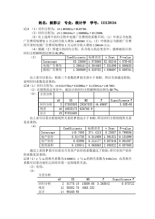
姓名:候彩云专业:统计学学号:11112011612,4 (1)回归方程为:y= 1.603865x1+ 88.63768;(2)回归方程为:y= 2.290184x1+ 1.300989x2+ 83.23009;(3)在上述两个回归方程中电视广告费用的系数不同;(1)中表示当电视广告费用每增加1万元时月收入增加1.603865万元;(2)中则表示当报纸广告费用不变时电视广告费用每增加1万元时月收入增加2.290184万元;(4)根据(2)所建立的回归方程,在月收入的总变差中,能够被估计的(5)由上表可以看出:检验三个系数的P值全部小于0.05,所以全部通过检验,说明回归系数是显著的;12.6(1)回归方程为:y= 0.814738x1+ 0.82098x2+ 0.135041x3+ 148.7005;(2(3)由上表可以看出检验线性关系的P值远小于0.05,所以回归方程的线性关系是显著的;(4)通过上表的P值可以看出只有房产估价的系数通过了检验,即只有房产估价的系数是显著的;12.9(1)y与x1的相关系数为0.308952;y与x2的相关系数为0.001214;由其相关系数可以看出他们之间存在着一定的线性关系;(2)有用;(3)方差分析df SS MS F Significance F 回归分析 2 31778.15 15889.08 3.265842 0.073722残差12 58382.78 4865.232总计14 90160.93通过上表可以看出用于检验线性关系的P值大于显著性水平0.05的值,表明购进价格和销售费用与销售价格之间没有显著性的线性关系;(4)判定系数R2=0.35246,表示在销售价格的总变差中,能够被购进价格和销售费用解释的比例为35.2%;这个结论与(2)中的结论基本上还是一致的,(5)x1与x2的相关系数为-0.85286,表明两者之间存在一定的线性关系;(6)由于购进价格与销售费用之间的相关系数不等于1,因此表明模型中存在多重共线性,我建议从模型中把销售价格这个变量剔除;。
第一章导论【重点】了解统计的科学涵义,明确统计学的学科性质及基本研究方法,掌握统计数据的特点及其不同类型,牢固掌握统计学的基本概念。
【难点】准确掌把数据不同类型,牢固掌握统计学的基本概念并结合实例分析。
思考题1.1什么是描述统计学、推断统计学?怎样理解描述统计学和推断统计学在探索事物数量规律性中的地位和作用?1.2统计学发展史上有哪几个主要学派?1.3“统计学”一词有哪几种含义?1.4什么是统计学?怎样理解统计学与统计数据的关系?1.5统计数据可分为哪几种类型?不同类型的数据各有什么特点?1.6举例说明总体、样本、参数、统计量、变量这几个概念。
练习题一、单项选择题1、指出下面的数据哪一个属于分类数据(D,)A、年龄B、工资C、汽车产量D、购买商品的支付方式(现金、信用卡、支票)2、指出下面的数据哪一个属于顺序数据(D,)A、年龄B、工资C、汽车产量D、员工对企业某项制度改革措施的态度(赞成、中立、反对)3、某研究部门准备在全市200万个家庭中抽取2000个家庭,据此推断该城市所有职工家庭的年人均收入,这项研究的统计量是(C,)A、2000个家庭B、200万个家庭C、2000个家庭的人均收入D、200万个家庭的人均收入4、了解居民的消费支出情况,则(B,)A、居民的消费支出情况是总体B、所有居民是总体C、居民的消费支出情况是总体单位D、所有居民是总体单位5、统计学研究的基本特点是(B)A、从数量上认识总体单位的特征和规律B、从数量上认识总体的特征和规律C、从性质上认识总体单位的特征和规律D、从性质上认识总体的特征和规律6、一家研究机构从IT从业者中随机抽取500人作为样本进行调查,其中60%的人回答他们的月收入在5000元以上,50%的回答他们的消费支付方式是使用信用卡。
这里的“月收入”是(C,)A、分类变量B、顺序变量C、数值型变量D、离散变量7、要反映我国工业企业的整体业绩水平,总体单位是(A)A、我国每一家工业企业B、我国所有工业企业C、我国工业企业总数D、我国工业企业的利润总额8、一项调查表明,在所抽取的1000个消费者中,他们每月在网上购物的平均消费是200元,他们选择在网上购物的主要原因是“价格便宜”。
第一章统计学及基本概念 1第二章数据的收集与整理 4第三章统计表与统计图7第四章数据的描述性分析 9第五章参数估计 12第六章假设检验 17第七章方差分析 21第八章非参数检验24第九章相关与回归分析27第十章多元统计分析 31第十一章时间序列分析35第十二章指数38第十二章指数38第十三章统计决策42第十四章统计质量管理45第一章统计学及基本概念1.1 统计的涵义(统计工作、统计资料和统计学)1.2 统计学的内容(统计学分类:理论统计学和应用统计学;描述统计学与推断统计学)1.3 统计学的发展史(学派与主要代表人物)1.4 数据类型(定类、定序、定距和定比;时间序列、截面数据和面板数据;绝对数、相对数、平均数)1.5 变量:连续与离散;确定与随机1.6 总体、样本与个体1.7 标志、指标及指标体系1.8 统计计算工具习题一、单项选择题1. 推断统计学研究()。
(知识点:1.2 答案:D)A.统计数据收集的方法B.数据加工处理的方法C.统计数据显示的方法D.如何根据样本数据去推断总体数量特征的方法2. 在统计史上被认为有统计学之名而无统计学之实的学派是()。
(知识点:1.3 答案:D) A.数理统计学派B.政治算术学派C.社会统计学派D.国势学派3. 下列数据中哪个是定比尺度衡量的数据()。
(知识点:1.4 答案:B)A.性别B.年龄C.籍贯D.民族4. 统计对现象总体数量特征的认识是()。
(知识点:1.6 答案:C)A.从定性到定量B.从定量到定性C.从个体到总体D.从总体到个体5. 调查10个企业职工的工资水平情况,则统计总体是()。
(知识点:1.6 答案:C)A.10个企业B.10个企业职工的全部工资C.10个企业的全部职工D.10个企业每个职工的工资6. 从统计总体中抽取出来作为代表这一总体的、由部分个体组成的集合体是().(知识点:1.6 答案:A)A. 样本B. 总体单位C. 个体D. 全及总体7. 三名学生期末统计学考试成绩分别为80分、85分和92分,这三个数字是()。
答案附在后面有一些(在题目上若要打印先把答案去掉)每单元后面都有答案第一章导论【重点】了解统计的科学涵义,明确统计学的学科性质及基本研究方法,掌握统计数据的特点及其不同类型,牢固掌握统计学的基本概念。
【难点】准确掌把数据不同类型,牢固掌握统计学的基本概念并结合实例分析。
思考题1.1什么是描述统计学、推断统计学?怎样理解描述统计学和推断统计学在探索事物数量规律性中的地位和作用?1.2统计学发展史上有哪几个主要学派?1.3“统计学”一词有哪几种含义?1.4什么是统计学?怎样理解统计学与统计数据的关系?1.5统计数据可分为哪几种类型?不同类型的数据各有什么特点?1.6举例说明总体、样本、参数、统计量、变量这几个概念。
练习题一、单项选择题1、指出下面的数据哪一个属于分类数据()A、年龄B、工资C、汽车产量D、购买商品的支付方式(现金、信用卡、支票)2、指出下面的数据哪一个属于顺序数据()A、年龄B、工资C、汽车产量D、员工对企业某项制度改革措施的态度(赞成、中立、反对)3、某研究部门准备在全市200万个家庭中抽取2000个家庭,据此推断该城市所有职工家庭的年人均收入,这项研究的统计量是()A、2000个家庭B、200万个家庭C、2000个家庭的人均收入D、200万个家庭的人均收入4、了解居民的消费支出情况,则()A、居民的消费支出情况是总体B、所有居民是总体C、居民的消费支出情况是总体单位D、所有居民是总体单位5、统计学研究的基本特点是()A、从数量上认识总体单位的特征和规律B、从数量上认识总体的特征和规律C、从性质上认识总体单位的特征和规律D、从性质上认识总体的特征和规律6、一家研究机构从IT从业者中随机抽取500人作为样本进行调查,其中60%的人回答他们的月收入在5000元以上,50%的回答他们的消费支付方式是使用信用卡。
这里的“月收入”是()A、分类变量B、顺序变量C、数值型变量D、离散变量7、要反映我国工业企业的整体业绩水平,总体单位是()A、我国每一家工业企业B、我国所有工业企业C、我国工业企业总数D、我国工业企业的利润总额8、一项调查表明,在所抽取的1000个消费者中,他们每月在网上购物的平均消费是200元,他们选择在网上购物的主要原因是“价格便宜”。
CHAPTER 1212.1 (a) When X = 0, the estimated expected value of Y is 2.(b) For each increase in the value X by 1 unit, you can expect an increase by an estimated 5 units in the value of Y .(c) ˆ2525(3)17YX =+=+= 12.2 (a) yes, (b) no,(c) no, (d) yes12.3 (a) When X = 0, the estimated expected value of Y is 16.(b) For each increase in the value X by 1 unit, you can expect a decrease in an estimated 0.5 units in the value of Y .(c) 13)6(5.0165.016ˆ=-=-=X Y12.4(a)(b) For each increase in shelf space of an additional foot, there is an expected increase in weekly sales of an estimated 0.074 hundreds of dollars, or $7.40. (c)042.2)8(074.045.1074.045.1ˆ=+=+=X Y, or $204.2012.5(a)Scatter Diagram0501001502002503003504004500100200300400500600700X, Reported (thousands)Y , A u d i t e d (t h o u s a n d s )(b)For each additional thousand units increase in reported newsstand sales, the mean audited sales will increase by an estimated 0.5719 thousand units.(c)()ˆ26.72400.5719400255.4788Y=+= thousands.12.6(a)(b) Partial Excel output:Coefficients Standard Error t Stat P-value Intercept -2.3697 2.0733 -1.1430 0.2610 Feet 0.0501 0.0030 16.5223 0.0000(c) The estimated mean amount of labor will increase by 0.05 hour for each additional cubic foot moved.(d)()ˆ 2.3697+0.050150022.6705Y=-=Scatter Diagram010********6070809002004006008001000120014001600XY12.7(a)(b) ˆ0.19120.0297YX =+ (c) For each increase of one additional pound, the estimated mean number of orders will increase by 29.7.(d) ()ˆ0.19120.029750015.043Y=+=thousands 12.8(a)Scatter Diagram010020030040050060070080090050100150200250X, Revenue (Millions of dollars)Y , V a l u e (M i l l i o n s o f d o l l a r s )(b)0246.2599b =-, 1 4.1897b =(c)For each additional million dollars increase in revenue, the mean annual value will increase by an estimated 4.1897 million dollars. Since revenue cannot be 0, the Y intercept has no practical interpretation. Also, since the Y intercept is outside the range of the observed values of the X variable, its interpretation should be made cautiously.(d)()ˆ246.2599 4.1897150382.2005Y=-+= million dollars.12.9(a)(b) X Y065.11.177ˆ+= (c) For each increase of 1 square foot in space, the expected monthly rental is estimated to increase by $1.065. Since X cannot be zero, 177.1 has no practical interpretation. (d) =+=+=)1000(065.11.177065.11.177ˆX Y $1242.10(e) An apartment with 500 square feet is outside the relevant range for the independent variable.(f)The apartment with 1200 square feet has the more favorable rent relative to size. Based on the regression equation, a 1200 square foot apartment would have anexpected monthly rent of $1455.10, while a 1000 square foot apartment would have an expected monthly rent of $1242.10.12.10 (a)12.10 (b) ˆ 6.0483 2.0191YX =+ cont. (c) For each increase of one additional Rockwell E unit in hardness, the estimated mean tensile strength will increase by 2.0191 thousand pounds per square inch.(d)()ˆ 6.0483 2.01913066.620Y=+= thousand pounds per square inch.12.11 80% of the variation in the dependent variable can be explained by the variation in the independent variable.12.12 SST = 40 and r 2 = 0.90. So, 90% of the variation in the dependent variable can be explained by the variation in the independent variable.12.13 r 2 = 0.75. So, 75% of the variation in the dependent variable can be explained by the variation in the independent variable.12.14 r 2 = 0.75. So, 75% of the variation in the dependent variable can be explained by the variation in the independent variable.12.15 Since SST = SSR + SSE and since SSE cannot be a negative number, SST must be at least as large as SSR . 12.16 (a)r 2 =2.05353.0025SSR SST == 0.684. So, 68.4% of the variation in the dependent variable can be explained by the variation in the independent variable.(b)0.308YXs ==== (c) Based on (a) and (b), the model should be very useful for predicting sales.12.17 (a) r 2 = 0.9015. So, 90.15% of the variation in audited newsstand sales can be explained by the variation in reported newsstand sales. (b) 42.1859YX s =(c) Based on (a) and (b), the model should be very useful for predicting audited sales.12.18 (a) r 2 = 0.8892. So, 88.92% of the variation in the dependent variable can be explained by the variation in the independent variable. (b) 5.0314YX s =(c) Based on (a) and (b), the model should be very useful for predicting labor hours.12.19 (a) r 2 = 0.9731. So, 97.31% of the variation in the dependent variable can be explained by the variation in the independent variable. (b) 0.7258YX s =(c)Based on (a) and (b), the model should be very useful for predicting the number of orders.12.20 (a) r 2 = 0.9424. So, 94.24% of the variation in value of a baseball franchise can be explained by the variation in its annual revenue. (b) 33.7876YX s =(c)Based on (a) and (b), the model should be very useful for predicting the value of a baseball franchise.12.21 (a) r 2 = 0.723. So, 72.3% of the variation in the dependent variable can be explained by the variation in the independent variable. (b) 6.194=YX s(c) Based on (a) and (b), the model should be very useful for predicting monthly rent.12.22 (a) r 2 = 0.4613. So, 46.13% of the variation in the dependent variable can be explained by the variation in the independent variable. (b) 9.0616YX s =(c)Based on (a) and (b), the model is only marginally useful for predicting tensile strength.12.23 A residual analysis of the data indicates no apparent pattern. The assumptions of regression appear to be met.12.24A residual analysis of the data indicates a pattern, with sizeable clusters ofconsecutive residuals that are either all positive or all negative. If the data is cross-sectional, this pattern indicates a violation of the assumption of linearity and a quadratic model should be investigated. If the data is time-series, the pattern indicates a violation of the assumption of independence of errors.12.25 (a)Reported Residual Plot-100-80-60-40-2002040600.0100.0200.0300.0400.0500.0600.0700.0ReportedR e s i d u a l sBased on the residual plot, there does not appear to be a pattern in the residual plot.(b)Normal Probability Plot-100-80-60-40-200204060Z ValueR e s i d u a l sBased on the residual plot, there appears to be some heteroscedasticity effect. The normal probability plot of the residuals indicates a departure from the normality assumption. The error distribution appears to be left-skewed.12.26 (a)Space Residual Plot-0.5-0.4-0.3-0.2-0.100.10.20.30.40.50510152025SpaceR e s i d u a l sBased on the residual plot, there does not appear to be a pattern in the residual plot. (b)Normal Probability Plot-0.5-0.4-0.3-0.2-0.100.10.20.30.40.5Z ValueR e s i d u a l sBased on the residual plot, there is not apparent heteroscedasticity effect. The normal probability plot of the residuals indicates a departure from the normality assumption.12.27 (a)Weight Residual Plot-2-1.5-1-0.500.511.50100200300400500600700800WeightR e s i d u a l sThe residual plot does not reveal any obvious pattern. So a linear fit appears to be adequate.(b)Normal Probability Plot-2-1.5-1-0.500.511.5Z ValueR e s i d u a l sThe residual plot does not reveal any possible violation of the homoscedasticity assumption. This is not a time series data, so you do not need to evaluate theindependence assumption. The normal probability plot shows that the distribution has a thicker left tail than a normal distribution but there is no sign of severe skewness.12.28 (a)Feet Residual Plot-15-10-5051015050010001500FeetR e s i d u a l sBased on the residual plot, there appears to be a nonlinear pattern in the residuals. A quadratic model should be investigated.(b)Normal Probability PlotZ ValueR e s i d u a l sThe assumptions of normality and equal variance do not appear to be seriously violated.12.29 (a)Size Residual Plot-500-400-300-200-100010020030040050005001000150020002500SizeR e s i d u a l sBased on a residual analysis of the residuals versus size, the model appears to be adequate. (b)Normal Probability Plot-500-400-300-200-1000100200300400500Z ValueR e s i d u a l sThe normal probability plot shows that the distribution has a thicker left tail than a normal distribution but there is no sign of severe skewness. The assumptions of regression do not appear to be seriously violated.12.30 (a)Revenue Residual Plot-80-60-40-20020406080100050100150200250RevenueR e s i d u a l sBased on the residual plot, there appears to be a nonlinear pattern in the residuals. A quadratic model should be investigated.(b)Normal Probability PlotZ ValueR e s i d u a l sThe normal probability plot of the residuals does not reveal significant departure from the normality assumption. The assumption of equal variance does not appear to be seriously violated.12.31 (a)The residual plot does not reveal any obvious pattern. So a linear fit appears to be adequate.(b)Normal Probability PlotZ ValueR e s i d u a l sThe residual plot does not reveal any possible violation of the homoscedasticity assumption. This is not a time series data, so you do not need to evaluate theindependence assumption. The normal probability plot shows that the distribution has a slightly thinner right tail than a normal distribution but there is no sign of severe skewness.12.32 (a)An increasing linear relationship exists.(b) There appears to be strong positive autocorrelation among the residuals.12.33 (a) There is no apparent pattern in the residuals over time.(b) D = 1.661>1.36. There is no evidence of positive autocorrelation among the residuals. (c) The data are not positively autocorrelated.12.34(a) No, it is not necessary to compute the Durbin-Watson statistic since the data have been collected for a single period for a set of stores.(b)If a single store was studied over a period of time and the amount of shelf space varied over time, computation of the Durbin-Watson statistic would be necessary.12.35 (a) b 0 = 169.455, b 1 = –1.8579(b) =-=-=)50(8579.1455.1698579.1455.169ˆX Y 76.56(c)(d) D = 1.18<1.27. There is evidence of positive autocorrelation among the residuals.(e)The plot of the residuals versus temperature indicates that positive residuals tend to occur for the lowest and highest temperatures in the data set. A nonlinear modelmight be more appropriate. The evidence of positive autocorrelation is another reason to question the validity of the model.12.36 (a) b 1 =201399.050.016112495626SSXY SSX == b 0 =()171.26210.01614393Y b X -=-= 0.458 (b)=+=+=)4500(0161.0458.00161.0458.0ˆX Y 72.908 or $72,908(c)(d)D =()212211243.2244599.0683ni i i nii e e e-==-=∑∑= 2.08>1.45. There is no evidence of positiveautocorrelation among the residuals.(e)Based on a residual analysis, the model appears to be adequate.12.37 (a)ˆ17.08335YX =- (b) ()ˆ17.083350.514.5833Y=-= seconds(c)There is no noticeable pattern in the plot.Residuals Plot-8-6-4-20246Time OrderR e s i d u a l s12.37 (d) H 0: There is no autocorrelation.cont. H 1: There is positive autocorrelation.PHStat output:Durbin-Watson CalculationsSum of Squared Difference of Residuals 238.4375L U H 0. There is no evidence of autocorrelation.(e)Based on the results of (c) and (d), there is no reason to question the validity of the model.12.38 (a) b 0 = –2.535, b 1 = 0.060728(b) =+-=+-=)83(060728.0535.2060728.0535.2ˆX Y 2.5054 or $2505.40(c)(d) D = 1.64>1.42. There is no evidence of positive autocorrelation among the residuals.(e)The plot of the residuals versus time period shows some clustering of positive and negative residuals for intervals in the domain, suggesting a nonlinear model might be better. Otherwise, the model appears to be adequate.12.39 (a)Scatter Diagram0501001502002501020304050X, Crude Oi Price (dollars/barrel)Y , G a s o l i n e P r i c e (c e n t s /g a l l o n )There appears to be a positive curvilinear relationship between crude oil price and gasoline price.(b) ()ˆ60.6944 2.8864YX =+ (c)Crude Oil Residual Plot-25-20-15-10-50510152025202530354045Crude OilR e s i d u a l sThere appears to be positive autocorrelation where clusters of positive residuals can be seen at the lower and upper range of the X value, and a cluster of negative residuals is apparent near the center of the X range. There also appears to be non-linear relationship between crude oil price and gasoline price.(d) 0.3161D =. 1.65L d =, 1.69U d =. Since D < 1.65, there is evidence of positive autocorrelation at 5% level of significance.(e)Based on the result of (c)-(d), the linear model and independent of errors assumptions do not appear to be valid.12.40 (a) 01:0H β= 11:0H β≠Test statistic: ()110/ 4.5/1.5 3.00b t b s =-==(b) With n = 18, df = 18 – 2 =16, 1199.216±=t .(c) Reject H 0. There is evidence that the fitted linear regression model is useful. (d) 111161116b b b t s b t s β-≤≤+)5.1(1199.25.4)5.1(1199.25.41+≤≤-β 68.732.11≤≤β12.41 (a) /60/160MSR SSR k ===/(1)40/18 2.222MSE SSE n k =--== 27222.2/60/===MSE MSR F (b) 1,18 4.41F =(c) Reject H 0. There is evidence that the fitted linear regression model is useful.(d) 2600.6100SSR r SST ===0.7746r ==-(e) 0:0H ρ=There is no correlation between X and Y . 1:0H ρ≠There is correlation between X and Y .d.f. = 18.Decision rule: Reject 0H if cal t >2.1009.Test statistic: 5.196t ===-.Since cal t = 5.196 >2.1009, reject 0H . There is enough evidence to conclude that the correlation between X and Y is significant.12.42 (a) 01:0H β= 11:0H β≠111100.074 4.65 2.22810.0159b b t t S β-===>=with 10 degrees of freedom for05.0=α. Reject H 0. There is enough evidence to conclude that the fitted linearregression model is useful.(b)()1120.074 2.22810.0159n b b t S -±=± 1094.00386.01≤≤β12.43 (a) 01:0H β=11:0H β≠PHStat output:CoefficientsStandard Errort Stat P-value Lower 95% Upper 95% Intercept26.7240 26.5425 1.00680.3435 -34.4832 87.9311 Reported0.5719 0.06688.55670.00000.41780.7260Since the p -value is essentially zero, reject H 0 at 5% level of significance. There is evidence of a linear relationship between reported sales and audited sales.(b)10.41780.7260β≤≤12.44 (a) 3416.5223 2.0322t t =>= for 05.0=α. Reject H 0. There is evidence that thefitted linear regression model is useful. (b) 10.04390.0562β≤≤12.45 (a) p -value is virtually 0 < 0.05. Reject H 0. There is evidence that the fitted linear regression model is useful. (b) 10.02760.0318β≤≤12.46 (a) 01:0H β=11:0H β≠PHStat output:CoefficientsStandard Errort Stat P-value Lower 95% Upper 95% Intercept-246.2599 26.0405 -9.4568 0.0000 -299.6015 -192.9183 Revenue4.1897 0.195721.40750.00003.78884.5906Since the p -value is essentially zero, reject H 0 at 5% level of significance. There is evidence of a linear relationship between annual revenue sales and franchise value. (b)13.7888 4.5906β≤≤12.47 (a) 0687.274.723=>=t t with 23 degrees of freedom for 05.0=α. Reject H 0. Thereis evidence that the fitted linear regression model is useful. (b) 10.7803 1.3497β≤≤12.48 (a) p -value = 7.26497E-06 < 0.05. Reject H 0. There is evidence that the fitted linear regression model is useful. (b) 11.2463 2.7918β≤≤12.49 (a)Sears, Roebuck and Company’s stock moves only 60.3% as much as the overall market and is much less volatile. LSI Logic’s stock moves 142.1% more than the overall market and is considered as extremely volatile. The stocks of Disney Company, Ford Motor Company and IBM, move 10.9%, 34% and 44.9%respectively more than the overall market and are considered somewhat more volatile than the market.(b)Investors can use the beta value as a measure of the volatility of a stock to assess its risk.12.50 (a)()()0% daily change in ULPIX 2.00% daily change in S&P 500 Index b =+ (b) If the S&P gains 30% in a year, the ULPIX is expected to gain an estimated 60%. (c) If the S&P loses 35% in a year, the ULPIX is expected to lose an estimated 70%.(d)Since the leverage funds have higher volatility and, hence, higher risk than the market, risk averse investors should stay away from these funds. Risk takers, on the other hand, will benefit from the higher potential gain from these funds.12.51 (a) r = -0.2810.(b) t = -1.0556, p -value = 0.3104 > 0.05. Do not reject H 0. There is not enoughevidence to conclude that there is a significant linear relationship between the retail price and the energy cost per year of medium-size top-freezer refrigerators.12.52 (a)r = –0.4014.(b)t = –1.8071, p -value = 0.089 > 0.05. Do not reject H 0. At the 0.05 level ofsignificance, there is no linear relationship between the turnover rate of pre-boarding screeners and the security violations detected.(c)There is not sufficient evidence to conclude that there is a linear relationship between the turnover rate of pre-boarding screeners and the security violations detected.12.53 (a)r = 0.3409.(b)t = 1.4506, p -value = 0.1662 > 0.05. Do not reject H 0. At the 0.05 level of significance, there is no linear relationship between the battery capacity and the digital-mode talk time.(c) There is not sufficient evidence to conclude that there is a linear relationship between the battery capacity and the digital-mode talk time.(d)No, the expectation that the cellphones with higher battery capacity have a higher talk time is not borne out by the data.12.54 (a)r = 0.4838(b)t = 2.5926, p -value = 0.0166 < 0.05. Reject H 0. At the 0.05 level of significance, there is a linear relationship between the cold-cranking amps and the price. (c) The higher the price of a battery is, the higher is its cold-cranking amps.(d)Yes, the expectation that batteries with higher cranking amps to have a higher price is borne out by the data.12.55 (a) When X = 2, 11)2(3535ˆ=+=+=X Y05.020)22(201)()(12122=-+=--+=∑=n i i i X X X X n h95% confidence interval: 05.011009.211ˆ18⋅⋅±=±h s t Y Y X|10.5311.47Y X μ≤≤(b)95% prediction interval: 05.111009.2111ˆ18⋅⋅±=+±h s t Y Y X28.84713.153X Y =≤≤12.56 (a) When X = 4, 17)4(3535ˆ=+=+=X Y25.020)24(201)()(12122=-+=--+=∑=n i i i X X X X n h95% confidence interval: 18ˆ17 2.10091YXY t s ±=±⋅|415.9518.05Y X μ=≤≤(b)95% prediction interval: 18ˆ17 2.10091YX Y t s ±=±⋅414.65119.349X Y =≤≤(c)The intervals in this problem are wider because the value of X is farther from X .12.57 (a)|400223.5000287.4577Y X μ=≤≤ (b)400153.0765357.8812X Y =≤≤ (c)Part (b) provides an interval prediction for the individual response given a specific value of the independent variable, and part (a) provides an interval estimate for the mean value given a specific value of the independent variable. Since there is much more variation in predicting an individual value than in estimating a mean value, a prediction interval is wider than a confidence interval estimate holding everything else fixed.12.58 (a)(2ˆ 2.042 2.22810.3081i n YX Y t S -±=±|81.7876 2.2964Y X μ=≤≤(b)(2ˆ 2.042 2.22810.3081i n YX Y t S -±=±81.3100 2.7740X Y =≤≤(c)Part (b) provides an interval prediction for the individual response given a specific value of the independent variable, and part (a) provides an interval estimate for the mean value given a specific value of the independent variable. Since there is much more variation in predicting an individual value than in estimating a mean value, a prediction interval is wider than a confidence interval estimate holding everything else fixed.12.59 (a)|50014.715015.3701Y X μ=≤≤ (b)50013.505916.5793X Y =≤≤ (c)Part (b) provides an interval prediction for the individual response given a specific value of the independent variable, and part (a) provides an interval estimate for the mean value given a specific value of the independent variable. Since there is much more variation in predicting an individual value than in estimating a mean value, a prediction interval is wider than a confidence interval estimate holding everything else fixed.12.60 (a)|50020.799024.5419Y X μ=≤≤ (b)50012.275533.0654X Y =≤≤ (c)Part (b) provides an interval prediction for the individual response given a specific value of the independent variable, and part (a) provides an interval estimate for the mean value given a specific value of the independent variable. Since there is much more variation in predicting an individual value than in estimating a mean value, a prediction interval is wider than a confidence interval estimate holding everything else fixed.12.61 (a)|10001153.01331.5Y X μ=≤≤(b) 1000829.91654.6X Y =≤≤(c) Part (b) provides an interval prediction for the individual response given a specificvalue of the independent variable, and part (a) provides an interval estimate for themean value given a specific value of the independent variable. Since there is muchmore variation in predicting an individual value than in estimating a mean value, aprediction interval is wider than a confidence interval estimate holding everythingelse fixed.12.62 (a)|150367.0757397.3254Y X μ=≤≤(b) 150311.3562453.0448X Y =≤≤(c) Part (b) provides an interval prediction for the individual response given a specificvalue of the independent variable, and part (a) provides an interval estimate for themean value given a specific value of the independent variable. Since there is muchmore variation in predicting an individual value than in estimating a mean value, aprediction interval is wider than a confidence interval estimate holding everythingelse fixed.12.63 (a)|30116.7082178.0564Y X μ=≤≤(b) 30111.5942183.1704X Y =≤≤(c) Part (b) provides an interval prediction for the individual response given a specificvalue of the independent variable, and part (a) provides an interval estimate for themean value given a specific value of the independent variable. Since there is muchmore variation in predicting an individual value than in estimating a mean value, aprediction interval is wider than a confidence interval estimate holding everythingelse fixed.12.64 The slope of the line, b 1, represents the estimated expected change in Y per unit change in X .It represents the estimated mean amount that Y changes (either positively or negatively) for a particular unit change in X . The Y intercept b 0 represents the estimated mean value of Y when X equals 0.12.65 The coefficient of determination measures the proportion of variation in Y that is explainedby the independent variable X in the regression model.12.66 The unexplained variation or error sum of squares (SSE) will be equal to zero only when theregression line fits the data perfectly and the coefficient of determination equals 1.12.67 The explained variation or regression sum of squares (SSR) will be equal to zero only whenthere is no relationship between the Y and X variables, and the coefficient of determination equals 0.12.68 Unless a residual analysis is undertaken, you will not know whether the model fit isappropriate for the data. In addition, residual analysis can be used to check whether theassumptions of regression have been seriously violated.12.69 The assumptions of regression are normality of error, homoscedasticity, and independence oferrors.12.70 The normality of error assumption can be evaluated by obtaining a histogram, box-and-whisker plot, and/or normal probability plot of the residuals. The homoscedasticityassumption can be evaluated by plotting the residuals on the vertical axis and the X variable on the horizontal axis. The independence of errors assumption can be evaluated by plotting the residuals on the vertical axis and the time order variable on the horizontal axis. This assumption can also be evaluated by computing the Durbin-Watson statistic.12.71 If the data in a regression analysis has been collected over time, then the assumption ofindependence of errors needs to be evaluated using the Durbin-Watson statistic.12.72 The confidence interval for the mean response estimates the mean response for a given Xvalue. The prediction interval estimates the value for a single item or individual.12.73 (a) There is a strong positive correlation between course average and cumulative GPA,and between total hits and hit consistency. There is a moderate positive correlationbetween course average and hit consistency, and between cumulative GPA and hitconsistency.(b) It is not surprising that cumulative GPA is strongly and positively related to courseaverage because course average in a course contributes to the cumulative GPA andboth measure the performance of a student. It is also not surprising that total hits andhit consistency are highly positively related because hit consistency contributes tototal hits. Hit consistency is positively related to both cumulative GPA and courseaverage because the more frequently a student visits the Internet site supporting acourse, the more current the student is in the course and presumably the better thestudent performs in the course.12.74 (a) b 0 = 24.84, b 1 = 0.14(b) 24.84 is the portion of estimated mean delivery time that is not affected by thenumber of cases delivered. For each additional case, the estimated mean deliverytime increases by 0.14 minutes.(c) 84.45)150(14.084.2414.084.24ˆ=+=+=X Y(d) No, 500 cases is outside the relevant range of the data used to fit the regressionequation.(e) r 2 = 0.972. So, 97.2% of the variation in delivery time can be explained by thevariation in the number of cases.(f) Based on a visual inspection of the graphs of the distribution of residuals and theresiduals versus the number of cases, there is no pattern. The model appears to beadequate.(g) 1009.288.2418=>=t t with 18 degrees of freedom for 05.0=α. Reject H 0.There is evidence that the fitted linear regression model is useful.(h) |15044.8846.80Y X μ=≤≤(i) 15041.5650.12X Y =≤≤(j) 1518.01282.01≤≤β12.75 (a)b 0 = –63.02, b 1 = 0.189 (b)For each additional incoming call, the estimated mean number of trade executions increases by 0.189. – 63.02 is the portion of the estimated mean number of trade executions that is not affected by the number of incoming calls. Since the Y intercept is outside the range of the observed values of the X variable, its interpretation should be made cautiously. (c)99.314)2000(189.002.63189.002.63ˆ=+-=+-=X Y (d)No, 5000 incoming calls is outside the relevant range of the data used to fit the regression equation. (e)r 2 = 0.630. So, 63.0% of the variation in the number of trade executions can be explained by the variation in the number of incoming calls. (f)Based on a visual inspection of the graphs of the distribution of residuals and the residuals versus the number of cases, there is no pattern. The model appears to be adequate. (g)D = 1.96 (h)D = 1.96>1.52. There is no evidence of positive autocorrelation. The model appears to be adequate. (i)0345.250.733=>=t t with 33 degrees of freedom for 05.0=α. Reject H 0. There is evidence that the fitted linear regression model is useful. (j)|2000302.07327.91Y X μ=≤≤ (k)2000253.76376.22X Y =≤≤ (l)2403.01377.01≤≤β12.76 (a)Scatter Diagram 020406080100120140020406080100Assessed Value ($000)S e l l i n g P r i c e ($000)b 0 = –44.172, b 1 = 1.78171 (b)Since the assessed value of a home cannot be zero, the intercept has no practical interpretation. -44.172 is the portion of estimated mean selling price that is not affected by the assessed value. For each additional dollar in assessed value, the estimated mean selling price increases by $1.78. (c)458.80)70(78171.1172.4478171.1172.44ˆ=+-=+-=X Y or $80,458 (d)r 2 = 0.926. 92.6% of the variation in selling price can be explained by the variation in the assessed value.。