FLUENT 多相流模型中文版资料

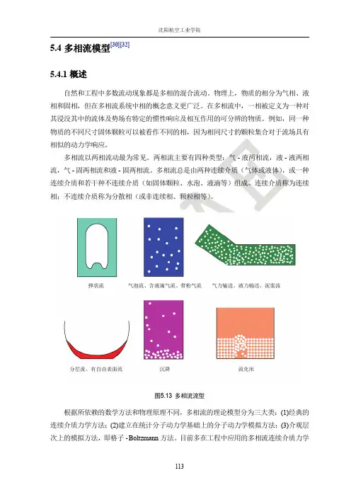
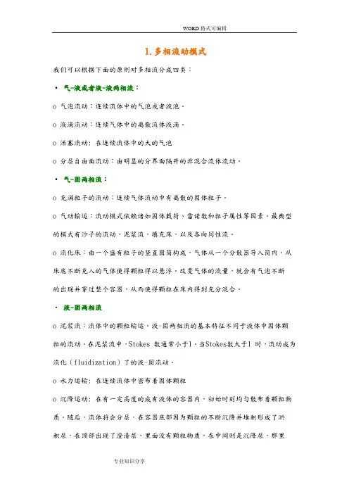
1.多相流动模式我们可以根据下面的原则对多相流分成四类：•气-液或者液-液两相流：o 气泡流动：连续流体中的气泡或者液泡。

o 液滴流动：连续气体中的离散流体液滴。

o 活塞流动: 在连续流体中的大的气泡o 分层自由面流动：由明显的分界面隔开的非混合流体流动。

•气-固两相流：o 充满粒子的流动：连续气体流动中有离散的固体粒子。

o 气动输运：流动模式依赖诸如固体载荷、雷诺数和粒子属性等因素。

最典型的模式有沙子的流动，泥浆流，填充床，以及各向同性流。

o 流化床：由一个盛有粒子的竖直圆筒构成，气体从一个分散器导入筒内。

从床底不断充入的气体使得颗粒得以悬浮。

改变气体的流量，就会有气泡不断的出现并穿过整个容器，从而使得颗粒在床内得到充分混合。

•液-固两相流o 泥浆流：流体中的颗粒输运。

液-固两相流的基本特征不同于液体中固体颗粒的流动。

在泥浆流中，Stokes 数通常小于1。

当Stokes数大于1 时，流动成为流化（fluidization）了的液-固流动。

o 水力运输: 在连续流体中密布着固体颗粒o 沉降运动: 在有一定高度的成有液体的容器内，初始时刻均匀散布着颗粒物质。

随后，流体将会分层，在容器底部因为颗粒的不断沉降并堆积形成了淤积层，在顶部出现了澄清层，里面没有颗粒物质，在中间则是沉降层，那里的粒子仍然在沉降。

在澄清层和沉降层中间，是一个清晰可辨的交界面。

•三相流 (上面各种情况的组合)各流动模式对应的例子如下：•气泡流例子：抽吸，通风，空气泵，气穴，蒸发，浮选，洗刷•液滴流例子：抽吸，喷雾，燃烧室，低温泵，干燥机，蒸发，气冷，刷洗•活塞流例子：管道或容器内有大尺度气泡的流动•分层自由面流动例子：分离器中的晃动，核反应装置中的沸腾和冷凝•粒子负载流动例子：旋风分离器，空气分类器，洗尘器，环境尘埃流动•风力输运例子：水泥、谷粒和金属粉末的输运•流化床例子：流化床反应器，循环流化床•泥浆流例子: 泥浆输运，矿物处理•水力输运例子：矿物处理，生物医学及物理化学中的流体系统•沉降例子：矿物处理2. 多相流模型FLUENT中描述两相流的两种方法:欧拉一欧拉法和欧拉一拉格朗日法，后面分别简称欧拉法和拉格朗日法。

FLUENT中文手册（简化版）本手册介绍FLUENT的使用方法，并附带了相关的算例。

下面是本教程各部分各章节的简略概括。

第一部分：☐开始使用：描述了FLUENT的计算能力以及它与其它程序的接口。

介绍了如何对具体的应用选择适当的解形式，并且概述了问题解决的大致步骤。

在本章中给出了一个简单的算例。

☐使用界面：描述用户界面、文本界面以及在线帮助的使用方法，还有远程处理与批处理的一些方法。

☐读写文件：描述了FLUENT可以读写的文件以及硬拷贝文件。

☐单位系统：描述了如何使用FLUENT所提供的标准与自定义单位系统。

☐使用网格：描述了各种计算网格来源，并解释了如何获取关于网格的诊断信息，以及通过尺度化（scale）、分区（partition）等方法对网格的修改。

还描述了非一致（nonconformal）网格的使用.☐边界条件：描述了FLUENT所提供的各种类型边界条件和源项，如何使用它们，如何定义它们等☐物理特性：描述了如何定义流体的物理特性与方程。

FLUENT采用这些信息来处理你的输入信息。

第二部分：☐基本物理模型：描述了计算流动和传热所用的物理模型（包括自然对流、周期流、热传导、swirling、旋转流、可压流、无粘流以及时间相关流）及其使用方法，还有自定义标量的信息。

☐湍流模型：描述了FLUENT的湍流模型以及使用条件。

☐辐射模型：描述了FLUENT的热辐射模型以及使用条件。

☐化学组分输运和反应流：描述了化学组分输运和反应流的模型及其使用方法，并详细叙述了prePDF 的使用方法。

☐污染形成模型：描述了NOx和烟尘的形成的模型，以及这些模型的使用方法。

第三部分：☐相变模拟：描述了FLUENT的相变模型及其使用方法。

☐离散相变模型：描述了FLUENT的离散相变模型及其使用方法。

☐多相流模型：描述了FLUENT的多相流模型及其使用方法。

☐移动坐标系下的流动：描述单一旋转坐标系、多重移动坐标系、以及滑动网格的使用方法。

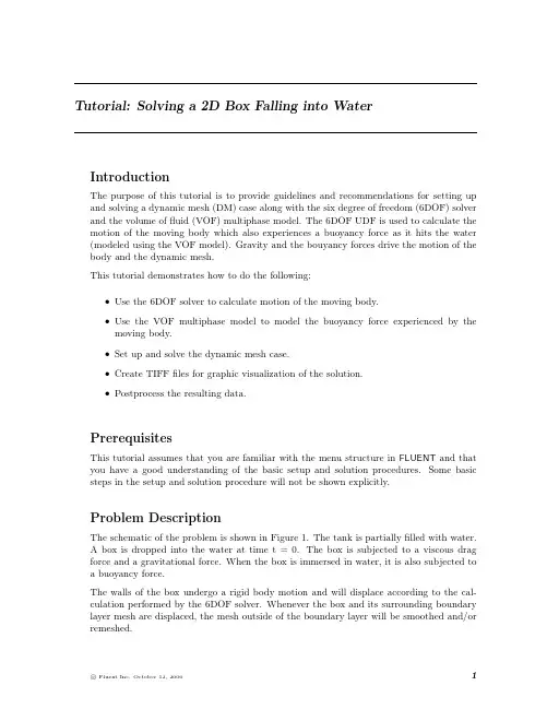
Tutorial:Solving a2D Box Falling into WaterIntroductionThe purpose of this tutorial is to provide guidelines and recommendations for setting up and solving a dynamic mesh(DM)case along with the six degree of freedom(6DOF)solver and the volume offluid(VOF)multiphase model.The6DOF UDF is used to calculate the motion of the moving body which also experiences a buoyancy force as it hits the water (modeled using the VOF model).Gravity and the bouyancy forces drive the motion of the body and the dynamic mesh.This tutorial demonstrates how to do the following:•Use the6DOF solver to calculate motion of the moving body.•Use the VOF multiphase model to model the buoyancy force experienced by themoving body.•Set up and solve the dynamic mesh case.•Create TIFFfiles for graphic visualization of the solution.•Postprocess the resulting data.PrerequisitesThis tutorial assumes that you are familiar with the menu structure in FLUENT and that you have a good understanding of the basic setup and solution procedures.Some basic steps in the setup and solution procedure will not be shown explicitly.Problem DescriptionThe schematic of the problem is shown in Figure1.The tank is partiallyfilled with water.A box is dropped into the water at time t=0.The box is subjected to a viscous dragforce and a gravitational force.When the box is immersed in water,it is also subjected toa buoyancy force.The walls of the box undergo a rigid body motion and will displace according to the cal-culation performed by the6DOF solver.Whenever the box and its surrounding boundary layer mesh are displaced,the mesh outside of the boundary layer will be smoothed and/or remeshed.Tutorial:Solving a2D Box Falling into WaterFigure1:Schematic of the ProblemPreparation1.Copy thefiles,6dof-mesh.msh.gz and6dof2d.c to your working folder.2.Create a subfolder named tiff-files to store the tifffiles created for postprocessingpurposes.3.Start the2D version of FLUENT.Tutorial:Solving a2D Box Falling into WaterSetup and SolutionStep1:Grid1.Read the meshfile6dof-mesh.msh.gz.File−→Read−→Case...2.Check the grid.Grid−→Check3.Display the grid(Figure2).Display−→Grid...Figure2:Grid DisplayTutorial:Solving a2D Box Falling into WaterStep2:Models1.Define the solver settings.Define−→Models−→Solver...(a)Select Unsteady from the Time list.(b)Retain the default selection of1st-Order Implicit for Unsteady Formulation.(c)Select the Green-Gauss Node Based option from the Gradient Option list.(d)Click OK to close the Solver panel.2.Define the multiphase model.Define−→Models−→Multiphase...(a)Select Volume of Fluid from the Model list.(b)Set Number of Phases to2.(c)Retain the default settings for VOF Scheme and Courant Number.(d)Enable Implicit Body Force formulation.(e)Click OK to close the Multiphase Model panel.3.Enable the standard k- turbulence model.Define−→Models−→Viscous...Step3:Compile the UDFDefine−→User-Defined−→Functions−→Compiled...1.Click the Add...button in the Source Files section to open the Select File panel.2.Select the sourcefile,6dof2d.c and click OK.3.Click Build to build the library.A Warning dialog box will open asking you to make sure that the UDF sourcefiles arein the same folder that contains the case and datafiles.(a)Click OK.FLUENT will compile the code and show the progress in the console.Monitor theprogress for compilation and linking errors.4.Click Load to load the newly created UDF library.Tutorial:Solving a2D Box Falling into WaterStep4:MaterialsDefine−→Materials...1.Retain the properties of air.2.Copy water-liquid(h2o<l>)from the FLUENT database.3.Modify the properties of water-liquid(h2o<l>).(a)Select user-defined from the Density drop-down list and water density from theUser-Defined Functions panel.(b)Select user-defined from the Speed of Sound drop-down list and water speed of soundfrom the User-Defined Functions panel.(c)Click Change/Create and close the Materials panel.Step5:PhasesDefine−→Phases...1.Define the primary phase(water).Define−→Phases...(a)Select phase-1and click Set...to open the Primary Phase panel.(b)Enter water for Name,.(c)Select water-liquid from the Phase Material drop-down list.(d)Click OK.2.Similarly,define the secondary phase(air),specifying air for Name and air for PhaseMaterial.Tutorial:Solving a2D Box Falling into WaterStep6:Operating ConditionsDefine−→Operating Conditions...1.Enter101325pascal for Operating Pressure.2.Enable Gravity.The panel expands to show additional inputs.3.Enter-9.81m/s2for Gravitational Acceleration in the Y direction.4.Enable Specified Operating Density and retain the default setting of1.225kg/m3forOperating Density.Step7:Boundary ConditionsDefine−→Boundary Conditions...1.Define the boundary conditions for tank outlet.(a)Set the boundary conditions for the mixture phase.i.Select mixture from the Phase drop-down list and click Set....ii.Select Intensity and Viscosity Ratio from the Turbulence Specification method drop-down list.iii.Enter1%for Backflow Turbulence Intensity and10for Backflow Turbulent Viscosity Ratio.iv.Click OK to close the Pressure Outlet panel.(b)Set the boundary conditions for the air phase.i.Select air from the Phase drop-down list and click Set....ii.Click the Multiphase tab and enter1for Backflow Volume Fraction.iii.Click OK to close the Pressure outlet panel.(c)Close the Boundary Conditions panel.Tutorial:Solving a2D Box Falling into Water Step8:Dynamic Mesh Setup1.Set the dynamic mesh parameters.Define−→Dynamic Mesh−→Parameters...(a)Enable Dynamic Mesh from the Models list.The panel expands to show additional inputs.(b)Enable Six DOF Solver from the Models list.(c)Enable Smoothing and Remeshing from the Mesh Methods list.(d)Enter0.5for Spring Constant Factor.(e)Click the Remeshing tab and set the remeshing parameters.Tutorial:Solving a2D Box Falling into Wateri.Enter0.056m for Minimum Length Scale and0.13m for Maximum LengthScale.The Minimum Length Scale and Maximum Length Scale can be obtained fromthe Mesh Scale Info panel.Click the Mesh Scale Info...button to open theMesh Scale Info panel.ii.Enter0.5for Maximum Cell Skewness.Gravitational acceleration must be specified in the Six DOF Solver tab.The nec-essary parameters have already been specified in the Operating Conditions panel.Hence,you need not do so again.(f)Click OK to close the Dynamic Mesh Parameters panel.2.Set up the moving zones.Define−→Dynamic Mesh−→Zones...Tutorial:Solving a2D Box Falling into Water(a)Create the dynamic zone,moving box.i.Select moving box from the Zone Names drop-down list.ii.Select Rigid Body from the Type list.iii.Select test box::libudf from the Six DOF UDF drop-down list.iv.Enable On from the Six DOF Solver Options group box.v.Click Create.FLUENT will create the dynamic zone moving box which will be available inthe Dynamic Zones list.(b)Create the dynamic zone,movingfluid.i.Select movingfluid from the Zone Names drop-down list.ii.Select Rigid Body from the Type list.iii.Select test box::libudf from the Six DOF UDF drop-down list.iv.Enable On and Passive from the Six DOF Solver Options group box.v.Click Create.FLUENT will create the dynamic zone movingfluid which will be available inthe Dynamic Zones list.Tutorial:Solving a2D Box Falling into Water(c)Close the Dynamic Mesh Zones panel.Step9:Mesh PreviewThe purpose of the preview is to verify the quality of the mesh yielded by the mesh motion parameters.Since theflow is not initialized,the motion of the box will be vertical due to gravity.1.Save the casefile,6dof-init.cas.gz.2.Display the grid.3.Preview the motion.Solve−→Mesh Motion...(a)Enter0.0005for Time Step Size.(b)Enter1000for Number of Time Steps.(c)Click Preview(Figures3and4).The motion is acceptable.(d)Close the Mesh Motion panel.4.Exit FLUENT without saving.Tutorial: Solving a 2D Box Falling into WaterGrid (Time=2.5000e-01)FLUENT 6.3 (2d, pbns, dynamesh, vof, ske, unsteady)Figure 3: Motion at t = 0.25 sGrid (Time=5.0000e-01)FLUENT 6.3 (2d, pbns, dynamesh, vof, ske, unsteady)Figure 4: Mesh Motion at t = 0.5 sc Fluent Inc. October 12, 200611Tutorial: Solving a 2D Box Falling into WaterStep 10: Solution Parameters 1. Start the 2D version of FLUENTand read the file 6dof-init.cas.gz. 2. Set the solution parameters. Solve −→ Controls −→Solution... (a) Select PRESTO! from the Pressure drop-down list in the Discretization group box. (b) Select Second Order Upwind for all other equations except Volume Fraction. (c) Retain the default discretization method of Geo-Reconstruct for Volume Fraction. (d) Select Coupled from the Pressure-Velocity Coupling drop-down list. (e) Enter 1000000 for Courant Number. (f) Enter 1.0 for Momentum and Pressure in the Explicit Relaxation Factors group box. (g) Enter 0.5 for Body Forces in the Under Relaxation Factor group box. (h) Click OK to close the Solution Controls panel. 3. Initialize the solution. Solve −→ Initialize −→Initialize... (a) Enter 0.001 m2 /s2 for Turbulence Kinetic Energy and 0.001 m2 /s3 for Turbulence Dissipation Rate. (b) Enter 1 for air Volume Fraction. (c) Click Init and close the Solution Initialization panel. 4. Create an adaption register for patching. Adapt −→Region... (a) Set the Input Coordinates as follows: Input Co-ordinates Xmin(m),Xmax(m) Ymin(m),Ymax(m) (b) Click Mark. (c) Close the Region Adaption panel. 5. Patch the air volume fraction. Solve −→ Initialize −→Patch... (a) Select air from the Phase drop-down list. (b) Select Volume Fraction from the Variable selection list. (c) Select hexahedron-r0 from the Registers to Patch selection list. (d) Retain the default Value of zero. (e) Click Patch. Values (-5,5) (-5,-1.5)12c Fluent Inc. October 12, 2006Tutorial: Solving a 2D Box Falling into Water(f) Close the Patch panel. 6. Enable the plotting of residuals. Solve −→ Monitors −→Residual... (a) Enable Plot in the Options list. (b) Enter 400 for number of iterations in the Plotting group box. 7. Define a surface monitor for Y Velocity. Solve −→ Monitors −→Surface... (a) Increase the number of Surface Monitors to 1. (b) Enable Plot, Print, and Write for monitor-1. (c) Select Time Step from the When drop-down list. (d) Click the Define... button to open the Define Surface Monitor panel. i. Select Area-Weighted Average from the Report Type drop-down list. ii. Select Flow Time from the X Axis drop-down list. iii. Retain the default setting of 1 for Plot Window. iv. Select Velocity... and Y Velocity from the Report of drop-down lists. v. Select moving box from the Surfaces selection list. vi. Enter 6dof yvel.out for File Name. vii. Click OK. (e) Click OK to close the Surface Monitors panel. 8. Activate Autosave option. File −→ Write −→Autosave... (a) Enter 100 for Autosave Case File Frequency. (b) Enter 100 for Autosave Data File Frequency. (c) Enable Overwrite Existing Files option. (d) Set the Maximum Number of Each File Type to 2. (e) Enter falling-box.gz for File Name. FLUENTwill append the timestep number so that each file created has a unique filename. (f) Click OK to close the Autosave Case/Data panel. Step 11: Set Hardcopy Options File −→Hardcopy... 1. Select TIFF from the Format list. 2. Select Color from the Coloring list. 13c Fluent Inc. October 12, 2006Tutorial: Solving a 2D Box Falling into Water3. Select Raster from the File Type list. 4. Enter 800 (pixels) for Width and 600 (pixels) for Height in the Resolution group box. 5. Click Apply and close the Graphics Hardcopy panel. Step 12: Define commands to create TIFF files for animation purposes Solve −→Execute Commands... 1. Set Defined Commands to 4. 2. Define the commands as follows:Command-1 Command-2 Command-3 Command-4Every 100 100 100 100When Time Step Time Step Time Step Time StepCommand display set-window 2 display contour water vof 0 1 display hard-copy "tiff-files/box-%t.tiff" display set-window 3Be sure to create the subfolder tiff-files before clicking the OK button. 1. Enable On for the four commands. 2. Click OK to close the Execute Commands panel. Step 13: Solution 1. Set the iteration parameters. (a) Enter 0.0005 for Time Step Size. (b) Enter 10000 for Number of Time Steps. (c) Set Max Iterations per Time Step to 50. (d) Click Iterate. Step 14: Postprocessing 1. Convert the TIFF files in the subfolder tiff-files to form an animation sequence for postprocessing purposes, using a third party software package like QuickTime or Fast Movie Player. Figures 5—24 show the contours of volume fraction of water at different time steps.14c Fluent Inc. October 12, 2006Tutorial: Solving a 2D Box Falling into Water1.00e+00 9.50e-01 9.00e-01 8.50e-01 8.00e-01 7.50e-01 7.00e-01 6.50e-01 6.00e-01 5.50e-01 5.00e-01 4.50e-01 4.00e-01 3.50e-01 3.00e-01 2.50e-01 2.00e-01 1.50e-01 1.00e-01 5.00e-02 0.00e+001.00e+00 9.50e-01 9.00e-01 8.50e-01 8.00e-01 7.50e-01 7.00e-01 6.50e-01 6.00e-01 5.50e-01 5.00e-01 4.50e-01 4.00e-01 3.50e-01 3.00e-01 2.50e-01 2.00e-01 1.50e-01 1.00e-01 5.00e-02 0.00e+00Contours of Volume fraction (water) (Time=2.5000e-01) FLUENT 6.3 (2d, pbns, dynamesh, vof, ske, unsteady)Contours of Volume fraction (water) (Time=5.0000e-01) FLUENT 6.3 (2d, pbns, dynamesh, vof, ske, unsteady)Figure 5: Contours at t = 0.25 sFigure 6: Contours at t = 0.5 s1.00e+00 9.50e-01 9.00e-01 8.50e-01 8.00e-01 7.50e-01 7.00e-01 6.50e-01 6.00e-01 5.50e-01 5.00e-01 4.50e-01 4.00e-01 3.50e-01 3.00e-01 2.50e-01 2.00e-01 1.50e-01 1.00e-01 5.00e-02 0.00e+001.00e+00 9.50e-01 9.00e-01 8.50e-01 8.00e-01 7.50e-01 7.00e-01 6.50e-01 6.00e-01 5.50e-01 5.00e-01 4.50e-01 4.00e-01 3.50e-01 3.00e-01 2.50e-01 2.00e-01 1.50e-01 1.00e-01 5.00e-02 0.00e+00Contours of Volume fraction (water) (Time=7.5001e-01) FLUENT 6.3 (2d, pbns, dynamesh, vof, ske, unsteady)Contours of Volume fraction (water) (Time=1.0000e+00) FLUENT 6.3 (2d, pbns, dynamesh, vof, ske, unsteady)Figure 7: Contours at t = 0.75 sFigure 8: Contours at t = 1.0 s1.00e+00 9.50e-01 9.00e-01 8.50e-01 8.00e-01 7.50e-01 7.00e-01 6.50e-01 6.00e-01 5.50e-01 5.00e-01 4.50e-01 4.00e-01 3.50e-01 3.00e-01 2.50e-01 2.00e-01 1.50e-01 1.00e-01 5.00e-02 0.00e+001.00e+00 9.50e-01 9.00e-01 8.50e-01 8.00e-01 7.50e-01 7.00e-01 6.50e-01 6.00e-01 5.50e-01 5.00e-01 4.50e-01 4.00e-01 3.50e-01 3.00e-01 2.50e-01 2.00e-01 1.50e-01 1.00e-01 5.00e-02 0.00e+00Contours of Volume fraction (water) (Time=1.2500e+00) FLUENT 6.3 (2d, pbns, dynamesh, vof, ske, unsteady)Contours of Volume fraction (water) (Time=1.5000e+00) FLUENT 6.3 (2d, pbns, dynamesh, vof, ske, unsteady)Figure 9: Contours t = 1.25 sFigure 10: Contours t = 1.5 sc Fluent Inc. October 12, 200615Tutorial: Solving a 2D Box Falling into Water1.00e+00 9.50e-01 9.00e-01 8.50e-01 8.00e-01 7.50e-01 7.00e-01 6.50e-01 6.00e-01 5.50e-01 5.00e-01 4.50e-01 4.00e-01 3.50e-01 3.00e-01 2.50e-01 2.00e-01 1.50e-01 1.00e-01 5.00e-02 0.00e+001.00e+00 9.50e-01 9.00e-01 8.50e-01 8.00e-01 7.50e-01 7.00e-01 6.50e-01 6.00e-01 5.50e-01 5.00e-01 4.50e-01 4.00e-01 3.50e-01 3.00e-01 2.50e-01 2.00e-01 1.50e-01 1.00e-01 5.00e-02 0.00e+00Contours of Volume fraction (water) (Time=1.7500e+00) FLUENT 6.3 (2d, pbns, dynamesh, vof, ske, unsteady)Contours of Volume fraction (water) (Time=1.9999e+00) FLUENT 6.3 (2d, pbns, dynamesh, vof, ske, unsteady)Figure 11: Contours at t = 1.75 sFigure 12: Contours at t = 2.0 s1.00e+00 9.50e-01 9.00e-01 8.50e-01 8.00e-01 7.50e-01 7.00e-01 6.50e-01 6.00e-01 5.50e-01 5.00e-01 4.50e-01 4.00e-01 3.50e-01 3.00e-01 2.50e-01 2.00e-01 1.50e-01 1.00e-01 5.00e-02 0.00e+001.00e+00 9.50e-01 9.00e-01 8.50e-01 8.00e-01 7.50e-01 7.00e-01 6.50e-01 6.00e-01 5.50e-01 5.00e-01 4.50e-01 4.00e-01 3.50e-01 3.00e-01 2.50e-01 2.00e-01 1.50e-01 1.00e-01 5.00e-02 0.00e+00Contours of Volume fraction (water) (Time=2.2499e+00) FLUENT 6.3 (2d, pbns, dynamesh, vof, ske, unsteady)Contours of Volume fraction (water) (Time=2.4999e+00) FLUENT 6.3 (2d, pbns, dynamesh, vof, ske, unsteady)Figure 13: Contours of at t = 2.25 sFigure 14: Contours at t = 2.5 s1.00e+00 9.50e-01 9.00e-01 8.50e-01 8.00e-01 7.50e-01 7.00e-01 6.50e-01 6.00e-01 5.50e-01 5.00e-01 4.50e-01 4.00e-01 3.50e-01 3.00e-01 2.50e-01 2.00e-01 1.50e-01 1.00e-01 5.00e-02 0.00e+001.00e+00 9.50e-01 9.00e-01 8.50e-01 8.00e-01 7.50e-01 7.00e-01 6.50e-01 6.00e-01 5.50e-01 5.00e-01 4.50e-01 4.00e-01 3.50e-01 3.00e-01 2.50e-01 2.00e-01 1.50e-01 1.00e-01 5.00e-02 0.00e+00Contours of Volume fraction (water) (Time=2.7499e+00) FLUENT 6.3 (2d, pbns, dynamesh, vof, ske, unsteady)Contours of Volume fraction (water) (Time=2.9999e+00) FLUENT 6.3 (2d, pbns, dynamesh, vof, ske, unsteady)Figure 15: Contours at t = 2.75 sFigure 16: Contours at t = 3.0 s16c Fluent Inc. October 12, 2006Tutorial: Solving a 2D Box Falling into Water1.00e+00 9.50e-01 9.00e-01 8.50e-01 8.00e-01 7.50e-01 7.00e-01 6.50e-01 6.00e-01 5.50e-01 5.00e-01 4.50e-01 4.00e-01 3.50e-01 3.00e-01 2.50e-01 2.00e-01 1.50e-01 1.00e-01 5.00e-02 0.00e+001.00e+00 9.50e-01 9.00e-01 8.50e-01 8.00e-01 7.50e-01 7.00e-01 6.50e-01 6.00e-01 5.50e-01 5.00e-01 4.50e-01 4.00e-01 3.50e-01 3.00e-01 2.50e-01 2.00e-01 1.50e-01 1.00e-01 5.00e-02 0.00e+00Contours of Volume fraction (water) (Time=3.2499e+00) FLUENT 6.3 (2d, pbns, dynamesh, vof, ske, unsteady)Contours of Volume fraction (water) (Time=3.4998e+00) FLUENT 6.3 (2d, pbns, dynamesh, vof, ske, unsteady)Figure 17: Contours at t = 3.25 sFigure 18: Contours at t = 3.5 s1.00e+00 9.50e-01 9.00e-01 8.50e-01 8.00e-01 7.50e-01 7.00e-01 6.50e-01 6.00e-01 5.50e-01 5.00e-01 4.50e-01 4.00e-01 3.50e-01 3.00e-01 2.50e-01 2.00e-01 1.50e-01 1.00e-01 5.00e-02 0.00e+001.00e+00 9.50e-01 9.00e-01 8.50e-01 8.00e-01 7.50e-01 7.00e-01 6.50e-01 6.00e-01 5.50e-01 5.00e-01 4.50e-01 4.00e-01 3.50e-01 3.00e-01 2.50e-01 2.00e-01 1.50e-01 1.00e-01 5.00e-02 0.00e+00Contours of Volume fraction (water) (Time=3.7498e+00) FLUENT 6.3 (2d, pbns, dynamesh, vof, ske, unsteady)Contours of Volume fraction (water) (Time=3.9998e+00) FLUENT 6.3 (2d, pbns, dynamesh, vof, ske, unsteady)Figure 19: Contours at t = 3.75 sFigure 20: Contours at t = 4.0 s1.00e+00 9.50e-01 9.00e-01 8.50e-01 8.00e-01 7.50e-01 7.00e-01 6.50e-01 6.00e-01 5.50e-01 5.00e-01 4.50e-01 4.00e-01 3.50e-01 3.00e-01 2.50e-01 2.00e-01 1.50e-01 1.00e-01 5.00e-02 0.00e+001.00e+00 9.50e-01 9.00e-01 8.50e-01 8.00e-01 7.50e-01 7.00e-01 6.50e-01 6.00e-01 5.50e-01 5.00e-01 4.50e-01 4.00e-01 3.50e-01 3.00e-01 2.50e-01 2.00e-01 1.50e-01 1.00e-01 5.00e-02 0.00e+00Contours of Volume fraction (water) (Time=4.2499e+00) FLUENT 6.3 (2d, pbns, dynamesh, vof, ske, unsteady)Contours of Volume fraction (water) (Time=4.5000e+00) FLUENT 6.3 (2d, pbns, dynamesh, vof, ske, unsteady)Figure 21: Contours at t = 4.25 sFigure 22: Contours at t = 4.5 sc Fluent Inc. October 12, 200617Tutorial: Solving a 2D Box Falling into Water1.00e+00 9.50e-01 9.00e-01 8.50e-01 8.00e-01 7.50e-01 7.00e-01 6.50e-01 6.00e-01 5.50e-01 5.00e-01 4.50e-01 4.00e-01 3.50e-01 3.00e-01 2.50e-01 2.00e-01 1.50e-01 1.00e-01 5.00e-02 0.00e+001.00e+00 9.50e-01 9.00e-01 8.50e-01 8.00e-01 7.50e-01 7.00e-01 6.50e-01 6.00e-01 5.50e-01 5.00e-01 4.50e-01 4.00e-01 3.50e-01 3.00e-01 2.50e-01 2.00e-01 1.50e-01 1.00e-01 5.00e-02 0.00e+00Contours of Volume fraction (water) (Time=4.7501e+00) FLUENT 6.3 (2d, pbns, dynamesh, vof, ske, unsteady)Contours of Volume fraction (water) (Time=5.0002e+00) FLUENT 6.3 (2d, pbns, dynamesh, vof, ske, unsteady)Figure 23: Contours at t = 4.75 sFigure 24: Contours at t = 5.0 sSummaryThis tutorial demonstrated the setup and solution of a dynamic mesh case along with the 6DOF solver and the VOF multiphase model. The 6DOF UDF was used to calculate the motion of the box dropped into the water. The TIFF files created in the tutorial can be used to provide a graphic visualization of the solution.18c Fluent Inc. October 12, 2006。

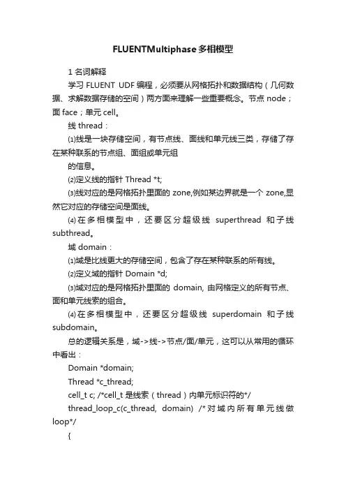
FLUENTMultiphase多相模型1 名词解释学习FLUENT UDF编程，必须要从网格拓扑和数据结构（几何数据、求解数据存储的空间）两方面来理解一些重要概念。

节点node；面face；单元cell。

线 thread：⑴线是一块存储空间，有节点线、面线和单元线三类，存储了存在某种联系的节点组、面组或单元组的信息。

⑵定义线的指针 Thread *t;⑶线对应的是网格拓扑里面的zone,例如某边界就是一个zone,显然它对应的存储空间是面线。

⑷在多相模型中，还要区分超级线superthread和子线subthread。

域 domain：⑴域是比线更大的存储空间，包含了存在某种联系的所有线。

⑵定义域的指针 Domain *d;⑶域对应的是网格拓扑里面的domain, 由网格定义的所有节点、面和单元线索的组合。

⑷在多相模型中，还要区分超级线superdomain和子线subdomain。

总的逻辑关系是，域->线->节点/面/单元，这可以从常用的循环中看出：Domain *domain;Thread *c_thread;cell_t c; /*cell_t 是线索（thread）内单元标识符的*/thread_loop_c(c_thread, domain) /*对域内所有单元线做loop*/{begin_c_loop(c, c_thread) /* 对线内所有单元做循环 */{……}end_c_loop(c, c_thread)}2 Multiphase-specific Data Types 多相专用数据类型除了在Data Types in ANSYS FLUENT中呈献的ANSYS FLUENT 专用的数据类型，还有一些专用于多相UDF的线（thread）和域（domain）数据结构。

当使用多相模型时(Mixture, VOF, or Eulerian)，这些数据结构用来存储混合相（mixture of all of the phases）和每个单独相的属性和变量。

FLUENT中文手册（简化版）本手册介绍FLUENT的使用方法，并附带了相关的算例。

下面是本教程各部分各章节的简略概括。

第一部分：☐开始使用：描述了FLUENT的计算能力以及它与其它程序的接口。

介绍了如何对具体的应用选择适当的解形式，并且概述了问题解决的大致步骤。

在本章中给出了一个简单的算例。

☐使用界面：描述用户界面、文本界面以及在线帮助的使用方法，还有远程处理与批处理的一些方法。

☐读写文件：描述了FLUENT可以读写的文件以及硬拷贝文件。

☐单位系统：描述了如何使用FLUENT所提供的标准与自定义单位系统。

☐使用网格：描述了各种计算网格来源，并解释了如何获取关于网格的诊断信息，以及通过尺度化（scale）、分区（partition）等方法对网格的修改。

还描述了非一致（nonconformal）网格的使用.☐边界条件：描述了FLUENT所提供的各种类型边界条件和源项，如何使用它们，如何定义它们等☐物理特性：描述了如何定义流体的物理特性与方程。

FLUENT采用这些信息来处理你的输入信息。

第二部分：☐基本物理模型：描述了计算流动和传热所用的物理模型（包括自然对流、周期流、热传导、swirling、旋转流、可压流、无粘流以及时间相关流）及其使用方法，还有自定义标量的信息。

☐湍流模型：描述了FLUENT的湍流模型以及使用条件。

☐辐射模型：描述了FLUENT的热辐射模型以及使用条件。

☐化学组分输运和反应流：描述了化学组分输运和反应流的模型及其使用方法，并详细叙述了prePDF 的使用方法。

☐污染形成模型：描述了NOx和烟尘的形成的模型，以及这些模型的使用方法。

第三部分：☐相变模拟：描述了FLUENT的相变模型及其使用方法。

☐离散相变模型：描述了FLUENT的离散相变模型及其使用方法。

☐多相流模型：描述了FLUENT的多相流模型及其使用方法。

☐移动坐标系下的流动：描述单一旋转坐标系、多重移动坐标系、以及滑动网格的使用方法。

1.多相流动模式我们可以根据下面的原则对多相流分成四类：•气-液或者液-液两相流：o 气泡流动：连续流体中的气泡或者液泡。

o 液滴流动：连续气体中的离散流体液滴。

o 活塞流动: 在连续流体中的大的气泡o 分层自由面流动：由明显的分界面隔开的非混合流体流动。

•气-固两相流：o 充满粒子的流动：连续气体流动中有离散的固体粒子。

o 气动输运：流动模式依赖诸如固体载荷、雷诺数和粒子属性等因素。

最典型的模式有沙子的流动，泥浆流，填充床，以及各向同性流。

o 流化床：由一个盛有粒子的竖直圆筒构成，气体从一个分散器导入筒内。

从床底不断充入的气体使得颗粒得以悬浮。

改变气体的流量，就会有气泡不断的出现并穿过整个容器，从而使得颗粒在床内得到充分混合。

•液-固两相流o 泥浆流：流体中的颗粒输运。

液-固两相流的基本特征不同于液体中固体颗粒的流动。

在泥浆流中，Stokes 数通常小于1。

当Stokes数大于1 时，流动成为流化（fluidization）了的液-固流动。

o 水力运输: 在连续流体中密布着固体颗粒o 沉降运动: 在有一定高度的成有液体的容器内，初始时刻均匀散布着颗粒物质。

随后，流体将会分层，在容器底部因为颗粒的不断沉降并堆积形成了淤积层，在顶部出现了澄清层，里面没有颗粒物质，在中间则是沉降层，那里的粒子仍然在沉降。

在澄清层和沉降层中间，是一个清晰可辨的交界面。

•三相流(上面各种情况的组合)各流动模式对应的例子如下：•气泡流例子：抽吸，通风，空气泵，气穴，蒸发，浮选，洗刷•液滴流例子：抽吸，喷雾，燃烧室，低温泵，干燥机，蒸发，气冷，刷洗•活塞流例子：管道或容器内有大尺度气泡的流动•分层自由面流动例子：分离器中的晃动，核反应装置中的沸腾和冷凝•粒子负载流动例子：旋风分离器，空气分类器，洗尘器，环境尘埃流动•风力输运例子：水泥、谷粒和金属粉末的输运•流化床例子：流化床反应器，循环流化床•泥浆流例子: 泥浆输运，矿物处理•水力输运例子：矿物处理，生物医学及物理化学中的流体系统•沉降例子：矿物处理2. 多相流模型FLUENT中描述两相流的两种方法:欧拉一欧拉法和欧拉一拉格朗日法，后面分别简称欧拉法和拉格朗日法。

20.通用多相流模型（General Multiphase Models）本章讨论了在FLUENT中可用的通用的多相流模型。

第18章提供了多相流模型的简要介绍。

第19章讨论了Lagrangian离散相模型，第21章讲述了FLUENT中的凝固和熔化模型。

20.1选择通用多相流模型（Choosing a General Multiphase Model）20.2VOF模型(Volume of Fluid(VOF)Model)20.3混合模型(Mixture Model)20.4欧拉模型(Eulerian Model)20.5气穴影响(Cavity Effects)20.6设置通用多相流问题(Setting Up a General Multiphase Problem)20.7通用多相流问题求解策略(Solution Strategies for General Multiphase Problems)20.8通用多相流问题后处理(Postprocessing for General Multiphase Problems)20.1选择通用的多相流模型（Choosing a General Multiphase Model）正如在Section 18.4中讨论过的，VOF模型适合于分层的或自由表面流，而mixture和Eulerian 模型适合于流动中有相混合或分离，或者分散相的volume fraction超过10%的情形。

（流动中分散相的volume fraction小于或等于10%时可使用第19章讨论过的离散相模型）。

为了在mixture模型和Eulerian模型之间作出选择，除了Section18.4中详细的指导外，你还应考虑以下几点：★如果分散相有着宽广的分布，mixture模型是最可取的。

如果分散相只集中在区域的一部分，你应当使用Eulerian模型。

★如果应用于你的系统的相间曳力规律是可利用的（either within FLUENT or through a user-defined function），Eulerian模型通常比mixture模型能给出更精确的结果。