计算机图形学第6章课后习题参考答案
- 格式:doc
- 大小:72.50 KB
- 文档页数:4
第一章测试1.计算机图形学产生图形,计算机图像学产生图像。
()A:对B:错答案:B2.下列哪项不属于计算机图形学的应用领域?()A:虚拟现实B:游戏实时显示C:科学计算可视化D:计算机辅助设计E:数字电影制作F:识别图片中的动物答案:F3.本课程将讲不讲解以下哪个内容?()A:动画生成B:真实感图像生成C:曲线生成D:游戏制作答案:D4.使用OPENGL画带颜色的直线,需要调用不同的函数,分别指定颜色和起始点坐标。
()A:错B:对答案:B5.在OPENGL中定义的结点仅包含位置信息。
()A:对B:错答案:B第二章测试1.四面体的表面建模中,可用四个三角形来描述四面体的表面,每个三角形包含三个点,因此,四面体中点的总个数为()。
A:12B:6C:4D:9答案:C2.三次BEZIER曲线有几个控制点?()A:3B:5C:4D:6答案:C3.三次BEZIER曲线经过几个控制点?()A:3B:4C:2D:1答案:C4.不经过Y轴的斜线绕Y轴旋转得到的曲面是()A:半球面B:球面C:柱面D:圆台面答案:B5.BEZIER曲线上的所有点都是由控制点经过插值得到的。
()A:错B:对答案:A第三章测试1.通过变换可以将单位圆变成长半轴2短轴0.5的椭圆,具体实施步骤是()。
A:水平方向做平移变换,竖值方向做平移变换B:水平方向做拉伸变换,竖值方向做平移变换C:水平方向做收缩变换,竖值方向做拉伸变换D:水平方向做拉伸变换,竖值方向做收缩变换答案:B2.变换前后二线夹角保持不变的保角变换有()A:镜像B:旋转C:平移D:缩放答案:D3.水平方向的剪切变换,如果表达为x’=ax+by y’=c x+dy,则有()。
A:b=1,c=1,d=0B:a=0,b=1,c=1C:a=1,b=0,d=1D:a=1,c=0,d=1答案:D4.正交变换不包括()。
A:剪切B:镜像C:旋转D:平移答案:A5.变换的复合运算不满足交换律。
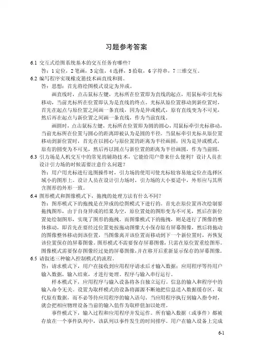
习题参考答案6.1交互式绘图系统基本的交互任务有哪些?答:1定位,2笔画,3定值,4选择,5拾取,6字符串,7三维交互。
6.2编写程序实现橡皮筋技术画直线和圆。
答:思想:首先将绘图模式设定为异或。
画直线时,点击鼠标左键,光标所在位置即为直线的起点,用鼠标牵引光标移动,当前光标所在位置即认为是直线的终点。
光标从原位置移动到新位置时,首先在起点与原位置之间画一条直线,因为是异或模式,原有直线变为不可见,然后再在起点与新位置之间画一条直线,作为当前直线。
画圆时,点击鼠标左键,光标所在位置即为圆的圆心,用鼠标牵引光标移动,当前光标所在位置与圆心的距离即被认为是圆的半径。
当鼠标牵引光标从原位置移动到新位置时,首先在以圆心与原位置的距离为半径画圆,因为是异或模式,原有的圆变为不可见,然后再以圆点与新位置的距离为半径画圆,作为当前圆。
6.3引力场是人机交互中的常见的辅助技术,它能给用户带来什么便利?设计人员在设计引力场的时候需要注意什么问题?答:用户用光标进行选图操作时,引力场的使用可使光标较容易地定位在选择区域小的图形上。
设计人员在设计引力场时,引力场的大小要适中,外形应与其所含图形的外形一致。
6.4图形模式和图像模式下,拖拽的处理方法有什么不同?答:图形模式下的拖拽是在异或的绘图模式下进行的。
首先在原位置再次绘制要拖拽图形,由于自身异或的结果为空,原位置处的图形变为不可见,然后在新位置处绘制图形,实现了图形的拖拽。
而图像模式下的拖拽,则是进行了图像的整体移动,即首先在要经过位置处按拖动图像大小保存原有屏幕图像,然后将拖动的图像整体移动到该位置,当图像离开该位置而移动到下一个新位置时,再恢复该位置保存的屏幕图像。
图形模式不需要保存屏幕图像,只需在原位置重绘图形。
图像模式需要保存图像经过处的屏幕图像,并在移开后重新显示保存的屏幕图像。
6.5请叙述三种输入控制模式的流程。
答:请求模式下,用户在接收到应用程序请求后才输入数据;应用程序等待用户输入数据,输入结束,才进行处理。
第一章1、试述计算机图形学研究的基本内容?答:见课本P5-6页的1.1.4节。
2、计算机图形学、图形处理与模式识别本质区别是什么?请各举一例说明。
答:计算机图形学是研究根据给定的描述,用计算机生成相应的图形、图像,且所生成的图形、图像可以显示屏幕上、硬拷贝输出或作为数据集存在计算机中的学科。
计算机图形学研究的是从数据描述到图形生成的过程。
例如计算机动画制作。
图形处理是利用计算机对原来存在物体的映像进行分析处理,然后再现图像。
例如工业中的射线探伤。
模式识别是指计算机对图形信息进行识别和分析描述,是从图形(图像)到描述的表达过程。
例如邮件分捡设备扫描信件上手写的邮政编码,并将编码用图像复原成数字。
3、计算机图形学与CAD、CAM技术关系如何?答:见课本P4-5页的1.1.3节。
4、举3个例子说明计算机图形学的应用。
答:①事务管理中的交互绘图应用图形学最多的领域之一是绘制事务管理中的各种图形。
通过从简明的形式呈现出数据的模型和趋势以增加对复杂现象的理解,并促使决策的制定。
②地理信息系统地理信息系统是建立在地理图形基础上的信息管理系统。
利用计算机图形生成技术可以绘制地理的、地质的以及其它自然现象的高精度勘探、测量图形。
③计算机动画用图形学的方法产生动画片,其形象逼真、生动,轻而易举地解决了人工绘图时难以解决的问题,大大提高了工作效率。
5、计算机绘图有哪些特点?答:见课本P8页的1.3.1节。
6、计算机生成图形的方法有哪些?答:计算机生成图形的方法有两种:矢量法和描点法。
①矢量法:在显示屏上先给定一系列坐标点,然后控制电子束在屏幕上按一定的顺序扫描,逐个“点亮”临近两点间的短矢量,从而得到一条近似的曲线。
尽管显示器产生的只是一些短直线的线段,但当直线段很短时,连成的曲线看起来还是光滑的。
②描点法:把显示屏幕分成有限个可发亮的离散点,每个离散点叫做一个像素,屏幕上由像素点组成的阵列称为光栅,曲线的绘制过程就是将该曲线在光栅上经过的那些像素点串接起来,使它们发亮,所显示的每一曲线都是由一定大小的像素点组成的。


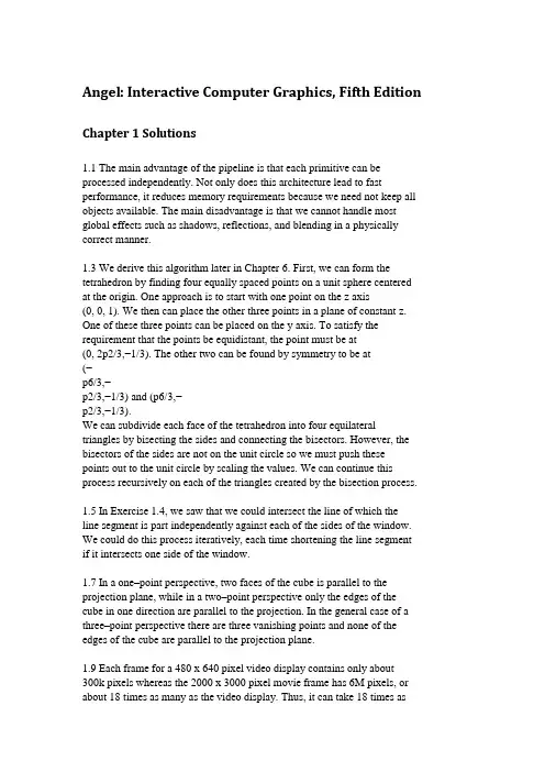
Angel: Interactive Computer Graphics, Fifth Edition Chapter 1 Solutions1.1 The main advantage of the pipeline is that each primitive can be processed independently. Not only does this architecture lead to fast performance, it reduces memory requirements because we need not keep all objects available. The main disadvantage is that we cannot handle most global effects such as shadows, reflections, and blending in a physically correct manner.1.3 We derive this algorithm later in Chapter 6. First, we can form the tetrahedron by finding four equally spaced points on a unit sphere centered at the origin. One approach is to start with one point on the z axis(0, 0, 1). We then can place the other three points in a plane of constant z. One of these three points can be placed on the y axis. To satisfy the requirement that the points be equidistant, the point must be at(0, 2p2/3,−1/3). The other two can be found by symmetry to be at(−p6/3,−p2/3,−1/3) and (p6/3,−p2/3,−1/3).We can subdivide each face of the tetrahedron into four equilateral triangles by bisecting the sides and connecting the bisectors. However, the bisectors of the sides are not on the unit circle so we must push thesepoints out to the unit circle by scaling the values. We can continue this process recursively on each of the triangles created by the bisection process.1.5 In Exercise 1.4, we saw that we could intersect the line of which theline segment is part independently against each of the sides of the window. We could do this process iteratively, each time shortening the line segment if it intersects one side of the window.1.7 In a one–point perspective, two faces of the cube is parallel to the projection plane, while in a two–point perspective only the edges of the cube in one direction are parallel to the projection. In the general case of a three–point perspective there are three vanishing points and none of the edges of the cube are parallel to the projection plane.1.9 Each frame for a 480 x 640 pixel video display contains only about300k pixels whereas the 2000 x 3000 pixel movie frame has 6M pixels, or about 18 times as many as the video display. Thus, it can take 18 times asmuch time to render each frame if there is a lot of pixel-level calculations.1.11 There are single beam CRTs. One scheme is to arrange the phosphors in vertical stripes (red, green, blue, red, green, ....). The major difficulty is that the beam must change very rapidly, approximately three times as fast a each beam in a three beam system. The electronics in such a system the electronic components must also be much faster (and more expensive). Chapter 2 Solutions2.9 We can solve this problem separately in the x and y directions. The transformation is linear, that is xs = ax + b, ys = cy + d. We must maintain proportions, so that xs in the same relative position in the viewport as x is in the window, hencex − xminxmax − xmin=xs − uw,xs = u + wx − xminxmax − xmin.Likewiseys = v + hx − xminymax − ymin.2.11 Most practical tests work on a line by line basis. Usually we use scanlines, each of which corresponds to a row of pixels in the frame buffer. If we compute the intersections of the edges of the polygon with a line passing through it, these intersections can be ordered. The first intersection begins a set of points inside the polygon. The second intersection leaves the polygon, the third reenters and so on.2.13 There are two fundamental approaches: vertex lists and edge lists. With vertex lists we store the vertex locations in an array. The mesh is represented as a list of interior polygons (those polygons with no otherpolygons inside them). Each interior polygon is represented as an array of pointers into the vertex array. To draw the mesh, we traverse the list of interior polygons, drawing each polygon.One disadvantage of the vertex list is that if we wish to draw the edges inthe mesh, by rendering each polygon shared edges are drawn twice. Wecan avoid this problem by forming an edge list or edge array, each elementis a pair of pointers to vertices in the vertex array. Thus, we can draw each edge once by simply traversing the edge list. However, the simple edge list has no information on polygons and thus if we want to render the mesh in some other way such as by filling interior polygons we must add somethingto this data structure that gives information as to which edges form each polygon.A flexible mesh representation would consist of an edge list, a vertex listand a polygon list with pointers so we could know which edges belong to which polygons and which polygons share a given vertex.2.15 The Maxwell triangle corresponds to the triangle that connects thered, green, and blue vertices in the color cube.2.19 Consider the lines defined by the sides of the polygon. We can assigna direction for each of these lines by traversing the vertices in acounter-clockwise order. One very simple test is obtained by noting thatany point inside the object is on the left of each of these lines. Thus, if we substitute the point into the equation for each of the lines (ax+by+c), we should always get the same sign.2.23 There are eight vertices and thus 256 = 28 possible black/white colorings. If we remove symmetries (black/white and rotational) there are14 unique cases. See Angel, Interactive Computer Graphics (Third Edition) or the paper by Lorensen and Kline in the references.Chapter 3 Solutions3.1 The general problem is how to describe a set of characters that might have thickness, curvature, and holes (such as in the letters a and q). Suppose that we consider a simple example where each character can be approximated by a sequence of line segments. One possibility is to use a move/line system where 0 is a move and 1 a line. Then a character can be described by a sequence of the form (x0, y0, b0), (x1, y1, b1), (x2, y2, b2), .....where bi is a 0 or 1. This approach is used in the example in the OpenGL Programming Guide. A more elaborate font can be developed by using polygons instead of line segments.3.11 There are a couple of potential problems. One is that the application program can map different points in object coordinates to the same point in screen coordinates. Second, a given position on the screen when transformed back into object coordinates may lie outside the user’s window.3.19 Each scan is allocated 1/60 second. For a given scan we have to take 10% of the time for the vertical retrace which means that we start to draw scan line n at .9n/(60*1024) seconds from the beginning of the refresh. But allocating 10% of this time for the horizontal retrace we are at pixel m on this line at time .81nm/(60*1024).3.25 When the display is changing, primitives that move or are removed from the display will leave a trace or motion blur on the display as the phosphors persist. Long persistence phosphors have been used in text only displays where motion blur is less of a problem and the long persistence gives a very stable flicker-free image.Chapter 4 Solutions4.1 If the scaling matrix is uniform thenRS = RS(α, α, α) = αR = SRConsider R x(θ), if we multiply and use the standard trigonometric identities for the sine and cosine of the sum of two angles, we findR x(θ)R x(φ) = R x(θ + φ)By simply multiplying the matrices we findT(x1, y1, z1)T(x2, y2, z2) = T(x1 + x2, y1 + y2, z1 + z2)4.5 There are 12 degrees of freedom in the three–dimensional affine transformation. Consider a point p = [x, y, z, 1]T that is transformed top_ = [x_y_, z_, 1]T by the matrix M. Hence we have the relationshipp_ = Mp where M has 12 unknown coefficients but p and p_ are known. Thus we have 3 equations in 12 unknowns (the fourth equation is simplythe identity 1=1). If we have 4 such pairs of points we will have 12equations in 12 unknowns which could be solved for the elements of M.Thus if we know how a quadrilateral is transformed we can determine theaffine transformation.In two dimensions, there are 6 degrees of freedom in M but p and p_ haveonly x and y components. Hence if we know 3 points both before and after transformation, we will have 6 equations in 6 unknowns and thus in two dimensions if we know how a triangle is transformed we can determine theaffine transformation.4.7 It is easy to show by simply multiplying the matrices that theconcatenation of two rotations yields a rotation and that the concatenationof two translations yields a translation. If we look at the product of arotation and a translation, we find that the left three columns of RT arethe left three columns of R and the right column of RT is the rightcolumn of the translation matrix. If we now consider RTR_ where R_ is arotation matrix, the left three columns are exactly the same as the leftthree columns of RR_ and the and right column still has 1 as its bottomelement. Thus, the form is the same as RT with an altered rotation (whichis the concatenation of the two rotations) and an altered translation.Inductively, we can see that any further concatenations with rotations and translations do not alter this form.4.9 If we do a translation by -h we convert the problem to reflection abouta line passing through the origin. From m we can find an angle by whichwe can rotate so the line is aligned with either the x or y axis. Now reflectabout the x or y axis. Finally we undo the rotation and translation so the sequence is of the form T−1R−1SRT.4.11 The most sensible place to put the shear is second so that the instance transformation becomes I = TRHS. We can see that this order makessense if we consider a cube centered at the origin whose sides are alignedwith the axes. The scale gives us the desired size and proportions. Theshear then converts the right parallelepiped to a general parallelepiped.Finally we can orient this parallelepiped with a rotation and place it wheredesired with a translation. Note that the order I = TRSH will work too.4.13R = R z(θz)R y(θy)R x(θx) =⎡⎢⎢⎢⎣cos θy cos θz cos θz sin θx sin θy −cos θx sin θz cos θx cos θz sin θy + sin θx sin θz 0cos θy sin θz cos θx cos θz + sin θx sin θy sin θz −cos θz sin θx + cos θx sin θy sin θz 0 −sin θy cos θy sin θx cos θx cos θy 00 0 0 1⎤⎥⎥⎥⎦4.17 One test is to use the first three vertices to find the equation of theplane ax + by + cz + d = 0. Although there are four coefficients in theequation only three are independent so we can select one arbitrarily ornormalize so that a2 + b2 + c2 = 1. Then we can successively evaluateax + bc + cz + d for the other vertices. A vertex will be on the plane if weevaluate to zero. An equivalent test is to form the matrix⎡⎢⎢⎢⎣1 1 1 1x1 x2 x3 x4y1 y2 y3 y4z1 z2 z3 z4⎤⎥⎥⎥⎦for each i = 4, ... If the determinant of this matrix is zero the ith vertex isin the plane determined by the first three.4.19 Although we will have the same number of degrees of freedom in theobjects we produce, the class of objects will be very different. For exampleif we rotate a square before we apply a nonuniform scale, we will shear the square, something we cannot do if we scale then rotate.4.21 The vector a = u ×v is orthogonal to u and v. The vector b = u ×a is orthogonal to u and a. Hence, u, a and b form an orthogonal coordinatesystem.4.23 Using r = cos θ2+ sin θ2v, with θ = 90 and v = (1, 0, 0), we find forrotation about the x-axisr =√22(1, 1, 0, 0).Likewise, for rotation about the y axisr =√22(1, 0, 1, 0).4.27 Possible reasons include (1) object-oriented systems are slower, (2)users are often comfortable working in world coordinates with higher-level objects and do not need the flexibility offered by a coordinate-free approach, (3) even a system that provides scalars, vectors, and points would have to have an underlying frame to use for the implementation. Chapter 5 Solutions5.1 Eclipses (both solar and lunar) are good examples of the projection of an object (the moon or the earth) onto a nonplanar surface. Any time a shadow is created on curved surface, there is a nonplanar projection. All the maps in an atlas are examples of the use of curved projectors. If the projectors were not curved we could not project the entire surface of a spherical object (the Earth) onto a rectangle.5.3 Suppose that we want the view of the Earth rotating about the sun. Before we draw the earth, we must rotate the Earth which is a rotation about the y axis. Next we translate the Earth away from the origin. Finally we do another rotation about the y axis to position the Earth in its desired location along its orbit. There are a number of interesting variants of this problem such as the view from the Earth of the rest of the solar system.5.5 Yes. Any sequence of rotations is equivalent to a single rotation abouta suitably chosen axis. One way to compute this rotation matrix is to form the matrix by sequence of simple rotations, such asR = RxRyRz.The desired axis is an eigenvector of this matrix.5.7 The result follows from the transformation being affine. We can also take a direct approach. Consider the line determined by the points(x1, y1, z1) and (x2, y2, z2). Any point along can be written parametrically as (_x1 + (1 − _)x2, _y1 + (1 − _)y2, _z1 + (1 − _)z2). Consider the simple projection of this point 1d(_z1+(1−_)z2) (_x1 + (1 − _)x2, _y1 + (1 − _)y2)which is of the form f(_)(_x1 + (1 − _)x2, _y1 + (1 − _)y2). This form describes a line because the slope is constant. Note that the function f(_) implies that we trace out the line at a nonlinear rate as _ increases from 0 to 1.5.9 The specification used in many graphics text is of the angles the projector makes with x,z and y, z planes, i.e the angles defined by the projection of a projector by a top view and a side view.Another approach is to specify the foreshortening of one or two sides of a cube aligned with the axes.5.11 The CORE system used this approach. Retained objects were kept in distorted form. Any transformation to any object that was defined with other than an orthographic view transformed the distorted object and the orthographic projection of the transformed distorted object was incorrect.5.15 If we use _ = _ = 45, we obtain the projection matrixP =266641 0 −1 00 1 −1 00 0 0 00 0 0 1377755.17 All the points on the projection of the point (x.y, z) in the direction dx, dy, dz) are of the form (x + _dx, y + _dy, z + _dz). Thus the shadow of the point (x, y, z) is found by determining the _ for which the line intersects the plane, that isaxs + bys + czs = dSubstituting and solving, we find_ =d − ax − by − czadx + bdy + cdz.However, what we want is a projection matrix, Using this value of _ we findxs = z + _dx =x(bdy + cdx) − dx(d − by − cz)adx + bdy + cdzwith similar equations for ys and zs. These results can be computed by multiplying the homogeneous coordinate point (x, y, z, 1) by the projection matrixM =26664bdy + cdz −bdx −cdx −ddx−ady adx + cdz −cdy −ddy−adz −bdz adx + bdy −ddz0 0 0 adx + bdy + cdz37775.5.21 Suppose that the average of the two eye positions is at (x, y, z) and the viewer is looking at the origin. We could form the images using the LookAt function twice, that isgluLookAt(x-dx/2, y, z, 0, 0, 0, 0, 1, 0);/* draw scene here *//* swap buffers and clear */gluLookAt(x+dx/2, y, z, 0, 0, 0, 0, 1, 0);/* draw scene again *//* swap buffers and clear */Chapter 6 Solutions6.1 Point sources produce a very harsh lighting. Such images are characterized by abrupt transitions between light and dark. The ambient light in a real scene is dependent on both the lights on the scene and the reflectivity properties of the objects in the scene, something that cannot be computed correctly with OpenGL. The Phong reflection term is not physically correct; the reflection term in the modified Phong model is even further from being physically correct.6.3 If we were to take into account a light source being obscured by an object, we would have to have all polygons available so as to test for this condition. Such a global calculation is incompatible with the pipeline model that assumes we can shade each polygon independently of all other polygons as it flows through the pipeline.6.5 Materials absorb light from sources. Thus, a surface that appears red under white light appears so because the surface absorbs all wavelengths of light except in the red range—a subtractive process. To be compatible with such a model, we should use surface absorbtion constants that define the materials for cyan, magenta and yellow, rather than red, green and blue. 6.7 Let ψ be the angle between the normal and the halfway vector, φ be the angle between the viewer and the reflection angle, and θ be the anglebetween the normal and the light source. If all the vectors lie in the same plane, the angle between the light source and the viewer can be computer either as φ + 2θ or as 2(θ + ψ). Setting the two equal, we find φ = 2ψ. Ifthe vectors are not coplanar then φ < 2ψ.6.13 Without loss of generality, we can consider the problem in two dimensions. Suppose that the first material has a velocity of light of v1 andthe second material has a light velocity of v2. Furthermore, assume thatthe axis y = 0 separates the two materials.Place a point light source at (0, h) where h > 0 and a viewer at (x, y)where y < 0. Light will travel in a straight line from the source to a point(t, 0) where it will leave the first material and enter the second. It willthen travel from this point in a straight line to (x, y). We must find the tthat minimizes the time travelled.Using some simple trigonometry, we find the line from the source to (t, 0)has length l1 = √h2 + t2 and the line from there to the viewer has length1l2 = _y2 + (x − t)2. The total time light travels is thus l1v1 + l2v2 .Minimizing over t gives desired result when we note the two desired sinesare sin θ1 = h√h2+t2 and sin θ2 = −y √(y2+(x−t)2 .6.19 Shading requires that when we transform normals and points, we maintain the angle between them or equivalently have the dot productp ·v = p_ ·v_ when p_ = Mp and n_ = Mp. If M T M is an identity matrix angles are preserved. Such a matrix (M−1 = M T ) is called orthogonal. Rotations and translations are orthogonal but scaling and shear are not.6.21 Probably the easiest approach to this problem is to rotate the givenplane to plane z = 0 and rotate the light source and objects in the sameway. Now we have the same problem we have solved and can rotate everything back at the end.6.23 A global rendering approach would generate all shadows correctly. Ina global renderer, as each point is shaded, a calculation is done to seewhich light sources shine on it. The projection approach assumes that wecan project each polygon onto all other polygons. If the shadow of a given polygon projects onto multiple polygons, we could not compute these shadow polygons very easily. In addition, we have not accounted for thedifferent shades we might see if there were intersecting shadows from multiple light sources.Chapter 7 Solutions7.1 First, consider the problem in two dimensions. We are looking for an _ and _ such that both parametric equations yield the same point, that isx(_) = (1 − _)x1 + _x2 = (1 − _)x3 + _x4,y(_) = (1 − _)y1 + _y2 = (1 − _)y3 + _y4.These are two equations in the two unknowns _ and _ and, as long as the line segments are not parallel (a condition that will lead to a division by zero), we can solve for _ _. If both these values are between 0 and 1, the segments intersect.If the equations are in 3D, we can solve two of them for the _ and _ where x and y meet. If when we use these values of the parameters in the two equations for z, the segments intersect if we get the same z from both equations.7.3 If we clip a convex region against a convex region, we produce the intersection of the two regions, that is the set of all points in both regions, which is a convex set and describes a convex region. To see this, consider any two points in the intersection. The line segment connecting them must be in both sets and therefore the intersection is convex.7.5 See Problem 6.22. Nonuniform scaling will not preserve the angle between the normal and other vectors.7.7 Note that we could use OpenGL to, produce a hidden line removed image by using the z buffer and drawing polygons with edges and interiors the same color as the background. But of course, this method was not used in pre–raster systems.Hidden–line removal algorithms work in object space, usually with either polygons or polyhedra. Back–facing polygons can be eliminated. In general, edges are intersected with polygons to determine any visible parts. Good algorithms (see Foley or Rogers) use various coherence strategies to minimize the number of intersections.7.9 The O(k) was based upon computing the intersection of rays with the planes containing the k polygons. We did not consider the cost of filling the polygons, which can be a large part of the rendering time. If we consider a scene which is viewed from a given point there will be some percentage of 1the area of the screen that is filled with polygons. As we move the viewer closer to the objects, fewer polygons will appear on the screen but eachwill occupy a larger area on the screen, thus leaving the area of the screen that is filled approximately the same. Thus the rendering time will be about the same even though there are fewer polygons displayed.7.11 There are a number of ways we can attempt to get O(k log k) performance. One is to use a better sorting algorithm for the depth sort. Other strategies are based on divide and conquer such a binary spatial partitioning.7.13 If we consider a ray tracer that only casts rays to the first intersection and does not compute shadow rays, reflected or transmitted rays, then the image produced using a Phong model at the point of intersection will be the same image as produced by our pipeline renderer. This approach is sometimes called ray casting and is used in volume rendering and CSG. However, the data are processed in a different order from the pipeline renderer. The ray tracer works ray by ray while the pipeline renderer works object by object.7.15 Consider a circle centered at the origin: x2 + y2 = r2. If we know thata point (x, y) is on the curve than, we also know (−x, y), (x,−y),(−x,−y), (y, x), (−y, x), (y,−x), and (−y,−x) are also on the curve. This observation is known as the eight–fold symmetry of the circle. Consequently, we need only generate 1/8 of the circle, a 45 degree wedge, and can obtain the rest by copying this part using the symmetries. If we consider the 45 degree wedge starting at the bottom, the slope of this curve starts at 0 and goes to 1, precisely the conditions used for Bresenham’s line algorithm. The tests are a bit more complex and we have to account for the possibility the slope will be one but the approach is the same as for line generation.7.17 Flood fill should work with arbitrary closed areas. In practice, we can get into trouble at corners if the edges are not clearly defined. Such can be the case with scanned images.7.19 Note that if we fill by scan lines vertical edges are not a problem. Probably the best way to handle the problem is to avoid it completely by never allowing vertices to be on scan lines. OpenGL does this by havingvertices placed halfway between scan lines. Other systems jitter the y value of any vertex where it is an integer.7.21 Although each pixel uses five rays, the total number of rays has only doubled, i.e. consider a second grid that is offset one half pixel in both the x and y directions.7.23 A mathematical answer can be investigated using the notion of reconstruction of a function from its samples (see Chapter 8). However, a very easy to see by simply drawing bitmap characters that small pixels lead to very unreadable characters. A readable character should have some overlap of the pixels.7.25 We want k levels between Imin and Imax that are distributed exponentially. Then I0 = Imin, I1 = Iminr,I2 = Iminr2, ..., Ik−1 = Imax = Iminrk−1. We can solve the last equation for the desired r = ( ImaxImin)1k−17.27 If there are very few levels, we cannot display a gradual change in brightness. Instead the viewer will see steps of intensity. A simple rule of thumb is that we need enough gray levels so that a change of one step is not visible. We can mitigate the problem by adding one bit of random noise to the least significant bit of a pixel. Thus if we have 3 bits (8 levels), the third bit will be noise. The effect of the noise will be to break up regions of almost constant intensity so the user will not be able to see a step because it will be masked by the noise. In a statistical sense the jittered image is a noisy (degraded) version of the original but in a visual sense it appears better.。
计算机图形学作业答案第一章序论第二章图形系统1.什么是图像的分辨率?解答:在水平和垂直方向上每单位长度(如英寸)所包含的像素点的数目。
2.计算在240像素/英寸下640×480图像的大小。
解答:(640/240)×(480/240)或者(8/3)×2英寸。
3.计算有512×512像素的2×2英寸图像的分辨率。
解答:512/2或256像素/英寸。
第三章二维图形生成技术1.一条直线的两个端点是(0,0)和(6,18),计算x从0变到6时y所对应的值,并画出结果。
解答:由于直线的方程没有给出,所以必须找到直线的方程。
下面是寻找直线方程(y =mx+b)的过程。
首先寻找斜率:m =⊿y/⊿x =(y2-y1)/(x2-x1)=(18-0)/(6-0) = 3接着b在y轴的截距可以代入方程y=3x+b求出 0=3(0)+b。
因此b=0,所以直线方程为y=3x。
2.使用斜截式方程画斜率介于0°和45°之间的直线的步骤是什么?解答:(1)计算dx:dx=x2-x1。
(2)计算dy:dy=y2-y1。
(3)计算m:m=dy/dx。
(4)计算b: b=y1-m×x1(5)设置左下方的端点坐标为(x,y),同时将x end设为x的最大值。
如果dx < 0,则x=x2、y=y2和x end=x1。
如果dx > 0,那么x=x1、y=y1和x end=x2。
(6)测试整条线是否已经画完,如果x > x end就停止。
(7)在当前的(x,y)坐标画一个点。
(8)增加x:x=x+1。
(9)根据方程y=mx+b计算下一个y值。
(10)转到步骤(6)。
3.请用伪代码程序描述使用斜截式方程画一条斜率介于45°和-45°(即|m|>1)之间的直线所需的步骤。
假设线段的两个端点为(x1,y1)和(x2,y2),且y1<y2int x = x1, y = y1;float x f, m = (y2-y1)/(x2-x1), b = y1-mx1;setPixel( x, y );/*画一个像素点*/while( y < y2 ) {y++;x f = ( y-b)/m;x = Floor( x f +0.5 );setPixel( x, y );}4.请用伪代码程序描述使用DDA算法扫描转换一条斜率介于-45°和45°(即|m|≤1)之间的直线所需的步骤。
第一章测试1.在几何造型系统中,描述物体的三维模型有三种,即线框模型、实体模型和________()。
A:色彩模型B:3D模型C:几何模型D:表面模型答案:D2.计算机图形是指由________和_________等非几何要素构成的,从现实世界中抽象出来的图或形()。
A:几何图形B:明暗、灰度(亮度)、色彩C:点、线、面、体等几何要素D:抽象元素答案:BC3.计算机图形学主要研究内容有()。
A:图形的处理B:图形的描述C:绘制D:交互处理答案:BCD4.计算机图形学的主要研究对象有()。
A:图形输入和控制的人机交互界面B:计算机环境下景物的几何建模方法C:几何模型的绘制技术D:模型的处理方法答案:ABD5.凡是能够在人的视觉系统中形成视觉印象的客观对象都称为图形。
()A:错B:对答案:B第二章测试1.根据视图所在的平面建立的坐标系为________()。
A:模型坐标系B:观察坐标系C:世界坐标系D:设备坐标系答案:B2.灰度等级为256级,分辨率为1024*1024的显示器,至少需要的帧缓存容量为 ( )A:512KBB:3MBC:1MBD:2MB答案:C3.计算机图形系统的主要功能有计算、_________等基本功能,它们相互协作,完成图形数据的处理过程()。
A:输出B:交互C:输入D:存储答案:ABCD4.一个计算机图形系统中计算功能有()。
A:图形的平移、旋转、投影、透视等几何变换B:图形之间相互关系的检测C:图形的描述、分析和设计D:曲线、曲面的生成答案:ABCD5.光栅化后的像素存放在缓存里的图形可自动输出到显示屏幕,完成场景的显示,人们就可以通过显示器观看图形。
()A:对B:错答案:B第三章测试1.a计算两物体各表面之间的交线 b建立新物体的边界表示 c对物体表面进行判定分类 d检查两物体是否相交。
如上,当物体采用边界表示时,它们之间的集合运算的具体实现步骤为()。
A:cdabB:cdbaC:dcabD:dacb答案:D2.设正则集合C表示A和B两物体的交,C=A∩B,b(A∩B)=b(A∩iB)∪(bB∩iA)∪(bA∩bB),则b(A∩bB)a-s表示bA∩bB中的______部分()。
《计算机图形学》习题与解答第一章概述1. 试描述你所熟悉的计算机图形系统的硬软件环境。
计算机图形系统是计算机硬件、图形输入输出设备、计算机系统软件和图形软件的集合。
例如:计算机硬件采用PC、操作系统采用windows2000,图形输入设备有键盘、鼠标、光笔、触摸屏等,图形输出设备有CRT、LCD等,安装3D MAX图形软件。
2. 计算机图形系统与一般的计算机系统最主要的差别是什么?3. 图形硬件设备主要包括哪些?请按类别举出典型的物理设备?图形输入设备:鼠标、光笔、触摸屏和坐标数字化仪,以及图形扫描仪等。
图形显示设备:CRT、液晶显示器(LCD)等。
图形绘制设备:打印机、绘图仪等。
图形处理器:GPU(图形处理单元)、图形加速卡等等。
4. 为什么要制定图形软件标准?可分为哪两类?为了提高计算机图形软件、计算机图形的应用软件以及相关软件的编程人员在不同计算机和图形设备之间的可移植性。
图形软件标准通常是指图形系统及其相关应用系统中各界面之间进行数据传送和通信的接口标准,另外还有供图形应用程序调用的子程序功能及其格式标准。
5. 请列举出当前已成为国际标准的几种图形软件标准,并简述其主要功能。
(1)CGI(Computer Graphics Interface),它所提供的主要功能集包括控制功能集、独立于设备的图形对象输出功能集、图段功能集、输入和应答功能集以及产生、修改、检索和显示以像素数据形式存储的光栅功能集。
(2)GKS(Graphcis Kernel System),提供了应用程序和图形输入输出设备之间的接口,包括一系列交互和非交互式图形设备的全部图形处理功能。
主要功能如下:控制功能、输入输出功能、变换功能、图段功能、询问功能等。
6. 试列举计算机图形学的三个应用实例。
(1)CAD/CAM(2)VISC(3)VR.第二章光栅图形学1. 在图形设备上如何输出一个点?为输出一条任意斜率的直线,一般受到哪些因素影响?若图形设备是光栅图形显示器,光栅图形显示器可以看作是一个像素的矩阵,光栅图形显示器上的点是像素点的集合。
计算机图形学答案(全面)第三章习题答案3.1 计算机图形系统的主要功能是什么?答:一个计算机图形系统应具有计算、存储、输入、输出、交互等基本功能,它们相互协作,完成图形数据的处理过程。
1. 计算功能计算功能包括:1)图形的描述、分析和设计;2)图形的平移、旋转、投影、透视等几何变换;3)曲线、曲面的生成;4)图形之间相互关系的检测等。
2. 存储功能使用图形数据库可以存放各种图形的几何数据及图形之间的相互关系,并能快速方便地实现对图形的删除、增加、修改等操作。
3. 输入功能通过图形输入设备可将基本的图形数据(如点、线等)和各种绘图命令输入到计算机中,从而构造更复杂的几何图形。
4. 输出功能图形数据经过计算后可在显示器上显示当前的状态以及经过图形编辑后的结果,同时还能通过绘图仪、打印机等设备实现硬拷贝输出,以便长期保存。
5. 交互功能设计人员可通过显示器或其他人机交互设备直接进行人机通信,对计算结果和图形利用定位、拾取等手段进行修改,同时对设计者或操作员输入的错误给以必要的提示和帮助。
3.2 阴极射线管由哪些部分组成?它们的功能分别是什么?答:CRT 主要由阴极、电平控制器(即控制极)、聚焦系统、加速系统、偏转系统和阳极荧光粉涂层组成,这六部分都在真空管内。
阴极(带负电荷)被灯丝加热后,发出电子并形成发散的电子云。
这些电子被电子聚集透镜聚焦成很细的电子束,在带正高压的阳极(实际为与加速极连通的CRT 屏幕内侧的石墨粉涂层,从高压入口引入阳极高电压)吸引下轰击荧光粉涂层,而形成亮点。
亮点维持发光的时间一般为20~40mS 。
电平控制器是用来控制电子束的强弱的,当加上正电压时,电子束就会大量通过,在屏幕上形成较亮的点,当控制电平加上负电压时,依据所加电压的大小,电子束被部分或全部阻截,通过的电子很少,屏幕上的点也就比较暗。
所以改变阴极和控制电平之间的电位差,就可调节电子束的电流密度,改变所形成亮点的明暗程度。
计算机图形学第二版(陆枫)课后习题集第一章绪论概念:计算机图形学、图形、图像、点阵法、参数法、图形的几何要素、非几何要素、数字图像处理;计算机图形学和计算机视觉的概念及三者之间的关系;计算机图形系统的功能、计算机图形系统的总体结构。
第二章图形设备图形输入设备:有哪些。
图形显示设备:CRT的结构、原理和工作方式。
彩色CRT:结构、原理。
随机扫描和光栅扫描的图形显示器的结构和工作原理。
图形显示子系统:分辨率、像素与帧缓存、颜色查找表等基本概念,分辨率的计算第三章交互式技术什么是输入模式的问题,有哪几种输入模式。
第四章图形的表示与数据结构自学,建议至少阅读一遍第五章基本图形生成算法概念:点阵字符和矢量字符;直线和圆的扫描转换算法;多边形的扫描转换:有效边表算法;区域填充:4/8连通的边界/泛填充算法;内外测试:奇偶规则,非零环绕数规则;反走样:反走样和走样的概念,过取样和区域取样。
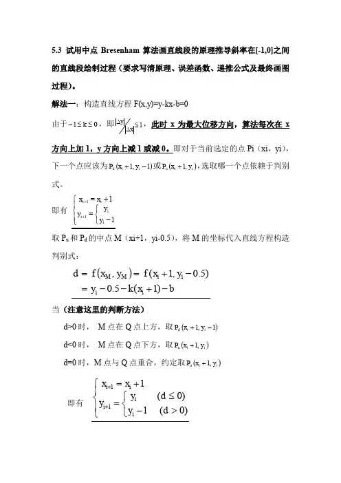
5.1.2 中点 Bresenham 算法(P109)5.1.2 改进 Bresenham 算法(P112)习题解答习题5(P144)5.3 试用中点Bresenham算法画直线段的原理推导斜率为负且大于1的直线段绘制过程(要求写清原理、误差函数、递推公式及最终画图过程)。
(P111)解: k<=-1 |△y|/|△x|>=1 y为最大位移方向故有构造判别式:推导d各种情况的方法(设理想直线与y=yi+1的交点为Q):所以有: y Q-kx Q-b=0 且y M=y Qd=f(x M-kx M-b-(y Q-kx Q-b)=k(x Q-x M)所以,当k<0,d>0时,M点在Q点右侧(Q在M左),取左点 P l(x i-1,y i+1)。
d<0时,M点在Q点左侧(Q在M右),取右点 Pr(x i,y i+1)。
d=0时,M点与Q点重合(Q在M点),约定取右点 Pr(x i,y i+1) 。
所以有递推公式的推导:d2=f(x i-1.5,y i+2)当d>0时,d2=y i+2-k(x i-1.5)-b 增量为1+k=d1+1+k当d<0时,d2=y i+2-k(x i-0.5)-b 增量为1=d1+1当d=0时,5.7 利用中点 Bresenham 画圆算法的原理,推导第一象限y=0到y=x圆弧段的扫描转换算法(要求写清原理、误差函数、递推公式及最终画图过程)。
第一章1、试述计算机图形学研究的基本内容?答:见课本P5-6页的1.1.4节。
2、计算机图形学、图形处理与模式识别本质区别是什么?请各举一例说明。
答:计算机图形学是研究根据给定的描述,用计算机生成相应的图形、图像,且所生成的图形、图像可以显示屏幕上、硬拷贝输出或作为数据集存在计算机中的学科。
计算机图形学研究的是从数据描述到图形生成的过程。
例如计算机动画制作。
图形处理是利用计算机对原来存在物体的映像进行分析处理,然后再现图像。
例如工业中的射线探伤。
模式识别是指计算机对图形信息进行识别和分析描述,是从图形(图像)到描述的表达过程。
例如邮件分捡设备扫描信件上手写的邮政编码,并将编码用图像复原成数字。
3、计算机图形学与CAD、CAM技术关系如何?答:见课本P4-5页的1.1.3节。
4、举3个例子说明计算机图形学的应用。
答:①事务管理中的交互绘图应用图形学最多的领域之一是绘制事务管理中的各种图形。
通过从简明的形式呈现出数据的模型和趋势以增加对复杂现象的理解,并促使决策的制定。
②地理信息系统地理信息系统是建立在地理图形基础上的信息管理系统。
利用计算机图形生成技术可以绘制地理的、地质的以及其它自然现象的高精度勘探、测量图形。
③计算机动画用图形学的方法产生动画片,其形象逼真、生动,轻而易举地解决了人工绘图时难以解决的问题,大大提高了工作效率。
5、计算机绘图有哪些特点?答:见课本P8页的1.3.1节。
6、计算机生成图形的方法有哪些?答:计算机生成图形的方法有两种:矢量法和描点法。
①矢量法:在显示屏上先给定一系列坐标点,然后控制电子束在屏幕上按一定的顺序扫描,逐个“点亮”临近两点间的短矢量,从而得到一条近似的曲线。
尽管显示器产生的只是一些短直线的线段,但当直线段很短时,连成的曲线看起来还是光滑的。
②描点法:把显示屏幕分成有限个可发亮的离散点,每个离散点叫做一个像素,屏幕上由像素点组成的阵列称为光栅,曲线的绘制过程就是将该曲线在光栅上经过的那些像素点串接起来,使它们发亮,所显示的每一曲线都是由一定大小的像素点组成的。
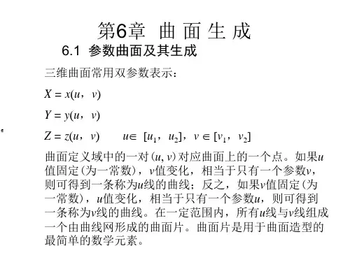
第六章
1.请简述朗伯(Lambert )定律。
设物体表面在P 点法线为N ,从P 点指向光源的向量为
L ,两者夹角为θ,则点P 处漫反射光的强度为:
I d =I p k d cos θ
式中 : I d ——表面漫反射光的亮度;
I p ——入射光的光亮度;
K d ——漫射系数(决定于表面材料及入射光的波长) 0≤K d ≤l ; θ——入射光线与法线间的夹角,0≤θ≤π/2。
并且,当物体表面垂直于入射光方向时(N 、L 方向一致)看上去最亮,而θ越来越大,接近90°时,则看上去越来越暗。
2.试写出实现哥罗德(Gouraud )明暗处理的算法伪代码。
deltaI = (i2 - i1) / (x2 - x1);
for (xx = x1; xx < x2; xx++)
{ int offset = row * CScene.screenW + xx;
if (z < CScene.zBuf[offset])
{ CScene.zBuf[offset] = z;
CScene.frameBuf[offset] = i1;
}
z += deltaZ; i1 += deltaI;
} 3. 在Phong 模型n s p d p a a V R K I N L K I K I I )()(⋅+⋅+=中,三项分别表示何含义?公式
中的各个符号的含义指什么?
三项分别代表环境光、漫反射光和镜面反射光。
a I 为环境光的反射光强,p I
为理想漫
反射光强,a K 为物体对环境光的反射系数,d K 为漫反射系数,s K 为镜面反射系数,n 为
高光指数,L 为光线方向,N 为法线方向,V 为视线方向,R 为光线的反射方向。
4.试写出实现Phong (冯)明暗方法的伪代码。
for (xx = x1; xx < x2; xx++)
{ int offset = row * CScene.screenW + xx;
if (z < CScene.zBuf[offset])
{ CScene.zBuf[offset] = z;
pt = face.findPtInWC(u,v);
float Ival = face.ptIntensity;
CScene.frameBuf[offset] = Ival;
}
u += deltaU;
z += deltaZ;
p1.add(deltaPt);
n1.add(deltaN);
}
5.请简述自身阴影的生成方法。
自身阴影生成过程如下:
(1)首先将视点置于光源位置,以光线照射方向作为观察方向,对在光照模型下的物体实施消隐算法,判别出在光照模型下的物体的“隐藏面”,并在数据文件中加以标识;
(2)然后按实际的视点位置和观察方向,对物体实施消隐算法,生成真正消隐后的立体图形;
(3)检索数据文件,核查消隐后生成的图形中,是否包含有在光照模型下的“隐藏面”。
如有,则加以阴影符号标识这些面。
6.试写出光线跟踪算法的C 语言描述。
/*TraceRay 的三个参数分别是起点start ,跟踪方向direction 和已跟踪的深度depth ,返回的是光线direction 的颜色。
*/
Color TraceRay(start,direction,depth)
V ector start,direction;
Int depth;
{
if (depth>MAX_DEPTH)
color=black;
else {
光线与物体求交,找出离start 最近的交点;
if (无交点)
color=背景色;
else {
local_color=用局部光照模型计算出的交点处的光强;
计算反射方向;
Reflected_color=TraceRay(交点,反射方向,depth+1);
计算折射方向;
Transmitted_color=TraceRay(交点,折射方向,depth+1);
Color= local_color+Reflected_color*Kr+Transmitted_color*Kt;
}
}
return color;
}
7.请简述计算机图形学所涉及到的纹理概念。
在计算机图形学中物体的表面细节称为纹理,包括颜色纹理与几何纹理。
颜色纹理主要是指光滑表面上附加花纹和图案,如墙面上的拼花图案、木质家具表面、塑料地板等。
几何纹理主要指景物表面在微观上呈现出的起伏不平,例如混凝土墙面、柑橘表皮等。
颜色纹理可用纹理映射(Texture Mapping)来描述,几何纹理可用一个扰动函数来描述。
8.写出从RGB颜色值到HSV值的转换算法。
RGB转化到HSV的算法:
max=max(R,G,B);
min=min(R,G,B);
if (R = max)
H = (G-B)/(max-min);
if (G = max)
H = 2 + (B-R)/(max-min);
if (B = max)
H = 4 + (R-G)/(max-min);
H = H * 60;
if (H < 0)
H = H + 360;
V=max(R,G,B);
S=(max-min)/max;
9.写出从HSV颜色值到RGB值的转换算法。
HSV转化到RGB的算法
if (s = 0)
R=G=B=v;
else
h /= 60;
i = int(h);
f =h – i;
a = v * ( 1 - s );
b = v * ( 1 - s * f );
c = v * ( 1 - s * (1 - f ) );
switch(i) {
case 0: R = v; G = c; B = a; break;
case 1: R = b; G = v; B = a; break;
case 2: R = a; G = v; B = c; break;
case 3: R = a; G = b; B = v; break;
case 4: R = c; G = a; B = v; break;
case 5: R = v; G = a; B = b;
}
10.写出从CMY颜色值到RGB值的转换表达式。
R = 255*(100-C)*(100-K)/10000;
G = 255*(100-M)*(100-K)/10000;
B = 255*(100-Y)*(100-K)/10000;
( C、M、Y取值在0-100之间)。