惯性导航作业
- 格式:docx
- 大小:20.62 KB
- 文档页数:3

惯性导航作业一、数据说明:1:惯导系统为指北方位的捷连系统。
初始经度为116.344695283度、纬度为39.975172度,高度h为30米。
初速度v0=[-9.993908270;0.000000000;0.348994967]。
2:jlfw中为600秒的数据,陀螺仪和加速度计采样周期分别为为1/100秒和1/100秒。
3:初始姿态角为[2 1 90](俯仰,横滚,航向,单位为度),jlfw.mat中保存的为比力信息f_INSc(单位m/s^2)、陀螺仪角速率信息wib_INSc(单位rad/s),排列顺序为一~三行分别为X、Y、Z向信息.4: 航向角以逆时针为正。
5:地球椭球长半径re=6378245;地球自转角速度wie=7.292115147e-5;重力加速度g=g0*(1+gk1*c33^2)*(1-2*h/re)/sqrt(1-gk2*c33^2);g0=9.7803267714;gk1=0.00193185138639;gk2=0.00669437999013;c33=sin(lat纬度);二、作业要求:1:可使用MATLAB语言编程,用MATLAB编程时可使用如下形式的语句读取数据:load D:\...文件路径...\jlfw,便可得到比力信息和陀螺仪角速率信息。
用角增量法。
2:(1) 以系统经度为横轴,纬度为纵轴(单位均要转换为:度)做出系统位置曲线图;(2) 做出系统东向速度和北向速度随时间变化曲线图(速度单位:m/s,时间单位:s);(3) 分别做出系统姿态角随时间变化曲线图(俯仰,横滚,航向,单位转换为:度,时间单位:s);以上结果均要附在作业报告中。
3:在作业报告中要写出“程序流程图、现阶段学习小结”,写明联系方式。
(注意程序流程图不是课本上的惯导解算流程,而是你程序分为哪几个模块、是怎样一步步执行的,什么位置循环等,让别人根据该流程图能够编出相应程序) (学习小结按条写,不用写套话) 4:作业以纸质报告形式提交,附源程序。
惯性导航岗位职责惯性导航岗位职责:惯性导航系统(Inertial Navigation System,简称INS)是一种基于惯性原理的导航系统,能够通过测量加速度和角速度的变化来确定飞行器的位置和运动状况。
在军事和民用航空领域中广泛使用,惯性导航工程师是负责设计、开发和维护惯性导航系统的专业人士。
下面是该岗位职责的详细描述:1. 设计惯性导航系统惯性导航工程师需要根据客户需求或项目要求,设计符合要求的惯性导航系统。
首先需要进行系统需求分析,确定设计目标和技术细节。
其次需要选择合适的传感器、计算单元和接口,进行系统硬件设计。
最后需要编写软件程序,实现系统的数据处理和控制功能。
2. 进行系统测试和优化设计好惯性导航系统之后,需要进行系统测试和优化。
这包括模拟环境下的系统测试和实际场景下的验证。
工程师需要对系统进行各种测试和分析,确定系统的精度、稳定性和可靠性等指标。
对测试结果进行分析和优化,确保系统满足客户需求和项目要求。
3. 维护和升级惯性导航系统惯性导航系统随着使用时间的推移和环境变化,可能会出现各种故障和问题。
工程师需要对系统进行维护和修复,确保系统能够正常运行。
同时,随着技术的不断发展,惯性导航系统也需要不断升级和改进。
工程师需要跟踪最新技术和市场趋势,为系统升级提供技术支持和建议。
4. 提供技术支持和培训惯性导航工程师需要与客户和团队密切合作,提供技术支持和解决方案。
对于一些复杂的问题,需要深入研究和解决。
此外,还需要为客户和团队提供相关的技术培训,帮助他们更好地使用和维护惯性导航系统。
总之,惯性导航工程师是惯性导航系统开发和运营的核心人才,需要具备扎实的技术功底和对航空领域的深刻理解。
他们需要设计、测试、维护和升级惯性导航系统,为客户提供技术支持和培训,确保系统能够稳定、高效、安全地运行。

导航系统1.简述捷联惯性系统中地理系到机体系的姿态阵bg C 其含义及其功能。
答:含义:导航坐标系g g g O x y z -到机体坐标系b b b O x y z -的一组欧拉角为,,θγψ,导航坐标系经过3次转动到机体坐标系。
g g g x y z 依次沿g O z -、'b O x -、''b O y -旋转角度-ψ、θ、γ后到b b b x y z 。
姿态矩阵中包含了机体的姿态角方位角ψ、俯仰角θ和横滚角γ。
功能:机体陀螺仪输出的角速度信息经过补偿后,积分得到机体坐标系与导航坐标系的姿态信息和姿态转移矩阵。
捷联惯导系统中,加速度计与载体固连,利用姿态阵完成加速度计输出信息从机体坐标到导航坐标的转换。
转换后的加速度计信息经过积分可得到机体在导航坐标系下的速度和位置。
2.画出并用式表达速度三角形(地速、控速、风速)及航迹角、航向角与偏流角之间的关系.答:风速:空气相对于地面的运动速度;空速:飞机相对于空气运动的速度;地速:飞机相对于地面的运动速度。
=+v v v 风地空航向角:机头在水平面投影与真北方向的夹角ϕ;偏流角:空速矢量和地速矢量之间的夹角,用δ表示;航迹角:飞机速度矢量在水平面投影与真北方向的夹角。
航向角ϕ加上偏流角δ等于地速v 地的方位角α。
v 地v 空v 风3.简述惯性导航系统、卫星导航系统、多普勒导航、塔康、VOR/DME 、天文导航其各自的基本工作原理、特点及误差特性。
答:一、惯性导航系统(1)工作原理以牛顿力学定律为基础,以陀螺仪和加速度计为敏感器件进行导航参数解算。
系统根据陀螺仪的输出建立导航坐标系,根据加速度计输出解算出运载体的速度和位置,从而实现姿态和航向解算. (2)特点惯性导航系统不需要任何外来信息,也不会向外辐射任何信息,仅依靠惯性器件就能全天候,全球性的自主三维定位和三维定向,同时具备自主性、隐蔽性和信息的完备性。
(3)误差特性误差随时间积累,短时间导航精度较高。
惯性导航技术在物理实验中的应用指南导语:在物理实验中,准确测量和记录物体的位置、速度和加速度是非常重要的。
惯性导航技术作为一种先进的测量方法,广泛应用于物理实验中,可以提供高精度和高稳定性的测量结果。
本文将为您介绍惯性导航技术在物理实验中的应用指南,帮助您更好地使用和理解该技术。
一、惯性导航技术概述惯性导航技术是利用惯性传感器来测量和跟踪物体的运动状态的一种方法。
主要包括3个方面的测量参数:加速度、角速度和姿态。
其中,加速度计可以测量物体在各个方向上的加速度变化;陀螺仪可以测量物体的角速度变化;磁强计可以测量物体的姿态变化。
这些测量参数可以通过导航算法计算出物体的位置和速度。
二、物理实验中的应用1. 弹道实验在弹道实验中,惯性导航技术可以用于测量炮弹的飞行轨迹。
通过陀螺仪测量炮弹的角速度变化,可以计算出炮弹的旋转角度和飞行方向。
结合加速度计和磁强计的测量结果,可以精确测量炮弹的速度和位置。
这些测量结果对于炮弹的准确定位和击中目标至关重要。
2. 自由落体实验在自由落体实验中,惯性导航技术可以用于测量物体下落过程中的加速度和速度。
通过加速度计测量物体的加速度变化,可以计算出重力加速度和物体的下落高度。
结合陀螺仪的测量结果,可以计算出物体的初始速度和离地点的时间。
这些测量结果可以帮助我们更好地理解自由落体物理学的规律。
3. 运动轨迹分析在运动轨迹分析实验中,惯性导航技术可以用于跟踪物体的位置和姿态变化。
通过磁强计测量物体的姿态变化,可以计算出物体的角度和方向。
结合陀螺仪和加速度计的测量结果,可以计算出物体的速度和加速度。
这些测量结果可以帮助我们更好地分析物体的运动轨迹和变化规律。
三、惯性导航技术的优势和挑战惯性导航技术具有高精度和高稳定性的优势,可以提供准确的测量结果。
同时,由于惯性传感器内部不需要外部参考,不受环境条件的限制,适用于各种复杂的实验场景。
然而,惯性导航技术也存在一些挑战,如漂移、噪声和精度损失等问题。

实验三惯性导航实验小组成员:杨曦陈魁吴航杨少帅一、 实验目的1、了解惯性导航设备;2、掌握惯性导航设备的物理连接;3、掌握惯性导航信息的处理方法;4、掌握惯性导航方法并学会用编程实现惯性导航算法。
二、 实验器材YH-5000AHRS ;工业控制计算机;数据采集软件; 稳压电源;串口连接线;三、 实验原理(1) 姿态解算基于四元数法解算姿态矩阵。
p j p i p l Q +++=21 (1)⎥⎥⎥⎦⎤⎢⎢⎢⎣⎡=⎥⎥⎥⎦⎤⎢⎢⎢⎣⎡⎥⎥⎥⎦⎤⎢⎢⎢⎣⎡--++----+++---+=⎥⎥⎥⎦⎤⎢⎢⎢⎣⎡b b b p b b b b p p p z y x C z y x p p p l lp p p lp p p lp p p p p p l lp p p lp p p lp p p p p p l z y x 222123213223113223212223212313212322212)(2)(2)(2)(2)(2)(2 (2) b pbQw Q 21= (3) 上述微分方程表示成矩阵形式:⎥⎥⎥⎥⎦⎤⎢⎢⎢⎢⎣⎡⎥⎥⎥⎥⎥⎦⎤⎢⎢⎢⎢⎢⎣⎡------=⎥⎥⎥⎥⎥⎦⎤⎢⎢⎢⎢⎢⎣⎡321321000021p p p l w w w w w w w w w w w w p p p l b pbxb pbyb pbz b pbx b pbz b pbyb pby b pbz b pbxb pbz b pbyb pbx(4) 初始四元数的确定计算如下:⎥⎥⎥⎥⎥⎥⎥⎥⎦⎤⎢⎢⎢⎢⎢⎢⎢⎢⎣⎡--++=⎥⎥⎥⎥⎦⎤⎢⎢⎢⎢⎣⎡2c o s 2c o s 2s i n 2s i n 2s i n 2c o s 2c o s 2s i n 2s i n 2s i n 2c o s 2c o s 2s i n 2c o s 2s i n 2c o s 2s i n 2c o s 2s i n 2s i n 2s i n 2c o s 2c o s 2co s )0(3)0(2)0()0(0000000000000000000000001γθϕγθϕγθϕγθϕγθϕγθϕγθϕγθϕG G G G G G G G p p p l (5) 用四阶龙格库塔法解(4)的微分方程;⎥⎥⎥⎦⎤⎢⎢⎢⎣⎡=333231232221131211T T T T T T T T T C p b 由p b C 中提取γϕλ,,G231sin T -=主λ 22211tan T T G -=主ϕ)(tan 33131T T --=主γ 从而可得到:主λλ=⎪⎩⎪⎨⎧<>+>><+=0,020,002122212222T T T T T GG G G πϕϕπϕϕ主主主⎩⎨⎧<>=0,)(-0331333T T sign T πγγγ (2) 速率位置解算将加速度测量的沿坐标系轴向的比力bib a 转换成沿着导航坐标系轴向的比力p ib a ,则速度方程为:p p epp ep p ib p ep g V w a V +⨯+Ω-=)2( 展开得到:⎪⎩⎪⎨⎧-+Ω-+Ω+=+Ω+Ω-=+Ω-Ω+=gV w V w a V V w V a V V w V a V p epy p epx p x p epx p epy p y p ibz pepz p epzp epx p x p epx p z p iby p epy p epzp epy p y p epy p z p ibx p epx )2()2()2(2)2(2 由于Ω,pep w 都很小,故而速度方程简化为:⎪⎩⎪⎨⎧-===ga V a V a V p ibz pepz piby p epy p ibxp epx用一阶欧拉法解,则:⎪⎩⎪⎨⎧+-=++=++=+)(*)()()(*)()(*)(t V T g a T t V t V T a T t V t V T a T t V p epz p ibz p epzpepy p iby p epy pepx p ibx p epx 其中T 为采样时间。
惯性导航仪的工作原理引言概述:惯性导航仪是一种用于飞行器、舰船、导弹等载具的导航设备,它能够通过测量载具的加速度和角速度来确定载具的位置、速度和方向。
惯性导航仪具有高精度、独立性强等优点,被广泛应用于航空航天领域。
一、惯性导航仪的基本原理1.1 惯性导航仪的加速度测量原理惯性导航仪内置加速度计,通过测量载具的加速度来确定载具的运动状态。
当载具发生加速度变化时,加速度计会产生相应的电信号,进而计算出载具的加速度值。
1.2 惯性导航仪的角速度测量原理惯性导航仪内置陀螺仪,通过测量载具的角速度来确定载具的旋转状态。
陀螺仪会产生相应的电信号,用于计算载具的角速度值。
1.3 综合加速度和角速度信息惯性导航仪会综合加速度和角速度信息,通过积分计算出载具的位置、速度和方向,从而实现导航功能。
二、惯性导航仪的误差补偿原理2.1 零偏误差补偿惯性导航仪存在零偏误差,需要进行零偏误差补偿。
通过定期校准零偏误差,可以提高导航仪的准确性。
2.2 温度漂移补偿惯性导航仪的性能会受到温度的影响,需要进行温度漂移补偿。
通过传感器内部的温度补偿电路,可以减小温度对导航仪的影响。
2.3 震动干扰抑制惯性导航仪在运动过程中会受到震动干扰,需要进行震动干扰抑制。
通过滤波算法和信号处理技术,可以减小震动对导航仪的影响。
三、惯性导航仪的工作模式3.1 静态模式在载具停止运动时,惯性导航仪处于静态模式。
此时,导航仪主要通过加速度计和陀螺仪测量载具的姿态和位置。
3.2 动态模式在载具运动时,惯性导航仪处于动态模式。
此时,导航仪主要通过积分计算出载具的位置、速度和方向。
3.3 切换模式惯性导航仪可以根据载具的运动状态自动切换不同的工作模式,以确保导航的准确性和稳定性。
四、惯性导航仪的应用领域4.1 航空领域惯性导航仪被广泛应用于飞机、直升机等航空器上,用于实现飞行导航和飞行控制。
4.2 舰船领域惯性导航仪也被应用于舰船上,用于实现航行导航和姿态控制。
惯导作业一、填空题1.惯性导航系统是一种不依赖任何外部信息、也不向外部辐射能量的______导航系统。
答案:自主式2.不依赖外界信息,只靠对载体本身的______、来完成导航任务的技术称做惯性导航,也称为自主式导航答案:惯性测量3. 加速度计其输出一般是______、,但在积分加速度计的情况下则输出为______、。
答案:速度、加速度4. 惯性器件就是测量载体______、和______、参数的传感器。
答案:线运动、角运动5. 加速度经过一次积分可以得到______,经过二次积分得到______。
答案:运动速度、运动距离6. 描述角运动的参数有______、______。
答案:姿态角、姿态角速度7. 描述线运动的参数有______、______、______。
答案:位移、速度、加速度8. 高速旋转的自由陀螺仪,当不受外力矩作用时,其主轴将保持它在空间的______方向不变。
答案:初始9. 由表观运动所引起的陀螺______偏离当地地垂线的误差,称之为陀螺仪的“表观误差”。
答案:自转轴二、单选题1.陀螺自转轴方向相对惯性空间保持不变,以地球作为参考基础,陀螺自转轴相对地球表面的转动,为()。
A.表观运动B.自转运动C.定轴运动D.进动运动答案:A三、多选题(每题1分)1.惯性导航系统的核心有()A.加速度计、B.陀螺仪C.导航计算机D.GPS答案:ABC2.惯性导航系统的基本组成()A.加速度计B.模拟某一坐标系的惯性平台C.导航计算机D.控制显示器答案:ABCD3.激光陀螺特点有哪些()。
A.抗干扰能力弱B.启动快C.动态特性较宽D.稳定性好答案:BCD4.关于组合导航系统,下列说法正确的是()。
A.提高导航系统的精度B.提高导航系统的可靠性C.提高导航系统的安全性D.启动快答案:ABC四、判断题1. 一个沿直线运动的载体,只要借助于加速度计测出它的加速度,那么,载体在任何时刻的速度和相对出发点的距离就可以实时地计算出来。

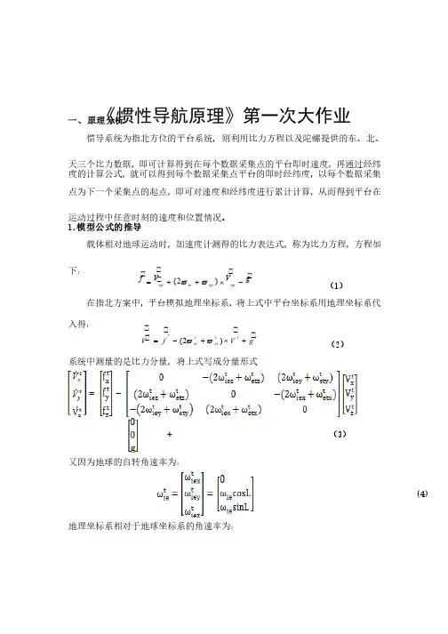
《惯性导航原理》第一次大作业一、 原理分析惯导系统为指北方位的平台系统,则利用比力方程以及陀螺提供的东、北、天三个比力数据,即可计算得到在每个数据采集点的平台即时速度,再通过经纬度的计算公式,就可以得到每个数据采集点平台的即时经纬度,以每个数据采集点为下一个采集点的起点,即可对速度和经纬度进行累计计算,从而得到平台在运动过程中任意时刻的速度和位置情况。
运动过程中任意时刻的速度和位置情况。
1.模型公式的推导载体相对地球运动时,载体相对地球运动时,加速度计测得的比力表达式,加速度计测得的比力表达式,加速度计测得的比力表达式,称为比力方程,称为比力方程,称为比力方程,方程如方程如下:下:g V V f epep ieep-´++=)2(vv (1)在指北方案中,平台模拟地理坐标系,将上式中平台坐标系用地理坐标系代入得:入得:t tt ett iettgV f V+´+-=)2(v v (2)系统中测量的是比力分量,将上式写成分量形式系统中测量的是比力分量,将上式写成分量形式=-+ (3) 又因为地球的自转角速率为:又因为地球的自转角速率为:(4)地理坐标系相对于地球坐标系的角速率为:地理坐标系相对于地球坐标系的角速率为:= (5)将(将(44)(5)两个式子带入()两个式子带入(33)式,即可得到如下方程组:)式,即可得到如下方程组:(6)2.速度计算作业要求只考虑水平通道,作业要求只考虑水平通道,因此只需要计算正东、因此只需要计算正东、因此只需要计算正东、正北两个方向的速度即可。
正北两个方向的速度即可。
正北两个方向的速度即可。
理理论上计算得到t x V 、t y V 后,再积分一次可得到速度值,即后,再积分一次可得到速度值,即ïîïíì+=+=òòt t y t y t ytt x t x tx V dt V V V dt V V 000但在本次计算过程中,三个方向的速度均是从零开始在各时间节点上的累加,并不是t的函数,因此速度计算可以由以下方程组实现:(7)此方程组表示了从第i 个采集点到第(个采集点到第(i+1i+1i+1)个采集点的速度递推公式。
Assignment ofInertial Technology《惯性技术》作业My Chinese NameMy Student ID 15S004001Autumn 2015Assignment 1: 2-DOF response simulationA 2-DOF gyro is subjected to a sinusoidal torque with amplitude of 4 g.cm and frequency of 10 Hz along its outer ring axis. The angular moment of its rotor is 10000 g.cm/s , and the angular inertias in its equatorial plane are both 4 g.cm/s 2. Please simulate the response of the gyro within 1 second, and present whatever you can discover or confirm from the result.In this simulation, we are going to discuss the response of a 2-DOF gyro to sinusoidal torque input. According to the transfer function of the 2-DOF gyro, the outputs can be expressed as:12222()()()()yx y x y x y J Hs M s M s J J s H s J J s H α=-++12222()()()()x yx x y x y J Hs M s M s J J s H s J J s H β=+++ The original system transfer function is a 2-input, 2-output coupling system. But the given input only exists one input, we can treat the system as 2 separate FIFO systemAs a consequence, we can establish the block diagram of the system in simulink in Fig 1.1. Substitute the parameters into the system and input, then we have the input signals as follow: 0,4sin(20)y ox M M t π==Then the inverse Laplace transform of the output equals the response of the gyro in timedomain as follows:0222200020222200()sin sin ()()()cos cos ()()ox a oxa x a x a ox ox a ox a a a a a M M t t t J J M M M t t t H H H ωαωωωωωωωωωβωωωωωωωω=-+--=+---Fig 1.1 The block diagram of the system in simulinkAnd the simulation results in time domain within 1 second are shown in the follwing pictures. Fig1.2 is the the output of outer ring ()t α. Fig1.3 is the output of inner ring ()t β. Fig1.4 is the trajectory of 2-DOF gyro ’s response to sinusoidal input. As we can see from the Fig1.3,there are obvious sawtooth wave in the output of the inner ring. It ’s a unexpected phenomenon in my original theoretical analysis.Fig1.2 The output of inner ring ()t βFig 1.3 The output of outer ring ()t αI believe the sawtooth wave is caused by the nutation. For the frequency of the nutation is obtained as010*******/3974e H rad s Hz J ω===≈, which is far higher than the frequencyof the applied sinusoidal torque , namely0a ωω .Fig 1.4 Trajectory of 2-DOF gyro ’s response to sinusoidal inputThe trajectory of 2-DOF gyro ’s response to sinusoidal input are shown in Fig1.4. As we can see, it ’s coupling of X and Y channel scope output. The overall shape is an ellipse, which is not perfect for there are so many sawteeth on the top of it.Note that the major axis of ellipse is in the direction of the forced procession, amplitude of which is 0ox M H ω, whereas the minor axis is in the direction of the torsion spring effects,with amplitude ox aM H ω.The nutation components are much smaller than that of the forced vibration, which can be eliminated to get the clear static response.22002220()sin sin ()cos (1cos )()ox oxaa x a ox ox oxa a a a a aM M t t t J H M M M t t t H H H αωωωωωωβωωωωωωω≈≈-≈-=--To prove it, we eliminate the effects of the nutation namely the quadratic term in the denominator and get Fig 1.5, which is a perfect ellipse. We can conclude that when input to the 2-DOF gyro is sinusoidal torque, the gyro will do an ellipse conical pendulum as a static response, including procession and the torsion spring effects, together with a high-frequency vibration as the dynamic response.Fig 1.5 Trajectory of the gyro’s response without nutationAssignment 2: Single-axis INS simulation2.1 description of the problemA magnetic levitation train is being tested along a track running north-south. It first accelerates and then cruises at a constant speed. Onboard is a single-axis platform INS, working in the way described by the courseware of Unit 5: Basic problems of INS. The motion informationand Earth parameters are shown in table 2-1, and the possible error sources are shown in Table2-2.Fig2.1 The sketch map of the single-axis INS problemYou are asked to simulate the operation of the INS within 10,000 seconds, and investigate,first one by one and then altogether, the impact of these error sources on the performance of theINS.The block diagram in the courseware might be of some help. However, there lurks aninconspicuous error, which you have to correct before you can obtain reasonable results.There are one core relevant formula, to get the specific form of its solution, we should substitute the unknown parameters.(1)()c N a y A K yga =∆++-Firstly, the input signal is accelerometer of the platform, and the velocity of the platform is the integration of the acceleration.0/p y y ydt yR ω=+=-⎰The acceleration along Yp may contains two parts:cos gsin g yp f y yααα=-≈- When accelerometer errors are concerned, the output of accelerometer will be:(1)N a yp N a K f A =++When gyro errors concerned:'(1)p g p K ωωε=++Onlyαis unknown:000[(1)]tg p t tp t K dt dtααωεϕϕω=+++-∆∆=⎰⎰And the reference block diagram and simulink block diagram are as follows in Fig2.2, Fig2.3. There is a small fault in the reference block, which is that the sign of the marked add operation should be positive instead of negative.The results of the simulation are shown in Fig 2.4 to Fig 2.13.Fig2.2 The reference block diagram in the courseware(unrectified)Fig2.3 The simulink block diagram for Assignment 22.2 results and analysis of the problemFig.2.4 real acceleration,velocity and displacement output without error sourcesKFig2.5 position bias when only accelerometer scale factor error exists0.0001aFig2.6 position bias output when only gyro scale factor error exists 0.0001g K =Fig2.7 position bias when only acceleromete bias error exists 20.0002/N A m s ∆=Fig2.8 position bias output when only initial velocity error exists 200.01/ym s ∆=Fig2.9 position bias output when only initial position error exists 010y m ∆=Fig2.10 position bias output bias when only gyro bias error exists 0.000000024240.00681/3/h rad s ε=︒=Fig2.11 position bias output when only initial platform misalignment angle exists0.000012120''345radα==Fig2.12 output considering all the error sourcesFig2.13 position bias output considering all error sourcesAs we can see in the above simulation results, if there is no error we can navigate the train ’s motion correctly, which comes from north to the south as shown in Fig2.4, beginning with an constant acceleration within 60 seconds then cruises at a constant speed, approximately 65 m/s. However, the situation will change a lot when different errors put into the simulation. The initial position error 010y m ∆= effects least as Fig.2.8, for this error doesn ’t enter into the closed loop and it won ’t influence the iterative process. The position bias is constant and can be negligible.In the second case, when the accelerometer scale factor error exists, 0.0001a K =, as shown in Fig2.5, the result are stable and almost accurate, the position bias is a sinusoidal output. So it is with the accelerometer bias error situation, 20.0002/N A m s ∆=, in Fig2.7, the initialvelocity error, 200.01/ym s ∆= in Fig2.9, and the initial platform misalignment angle, 05''α=, in Fig2.11. However, the influence degrees of the different factors are not in the samemagnitude. The accelerometer scale factor influences the least with magnitude of 5, then the initial velocity larger magnitude of 8, and the accelerometer bias magnitude of 25. The influence of the initial platform misalignment angle is much more significant with a magnitude of 150. All the navigation bias in the second kind case is sinusoidal, which means they ’re limited and negligible as time passes by.In the third case, such as the gyro scale factor error situation, 0.0001g K =, in Fig2.6, and the gyro bias error,0.01/h ε=︒, results in Fig2.10, effects the most significant, the trajectory of the navigation disvergence accumulated as time goes. The position bias is a combination of sinusoidal signal and ramp signal. They also show that the longitudinal and distance errors resulted from gyro drifts are not convergent in time. It means the errors in the gyroscope do most harm to our navigation. And due to the significant influence of the gyro bias errors and the gyroscope scale factor error, results considering all the error sources disverge, and the navigationposition of the motion will be away from the real motion after a enough long time, as shown in Fig2.10. The gyro bias error is the most significant effect factor of all errors. By the time of 10000s, it has reaches 1600m, and it’s nearly the quantity of the position bias considering all error sources. Through contrasting all the results, We can conclude that the gyro bias error is the main component of the whole position bias.Impression of the Whole simulation experimentThrough contrasting all the results, We can conclude that the gyro bias error is the main component of the whole position bias, and the the gyro bias or the drift error do most harm to our navigation. So it is a must for us to weaken or eliminate it anyway. In spite of all the disadvantages discussed above, the INS still shows us a relatively accurate results of single-axis navigation.Assignment 3: SINS simulation3.1 Task descriptionA missile equipped with SINS is initially at the position of 46o NL and 123 o EL, stationary on a launch pad. Three gyros, GX, GY, GZ, and three accelerometers, AX, AY, AZ, are installed along the axes Xb, Yb, Zb of its body frame respectively.Case 1: stationary testThe body frame of the missile initially coincides with the geographical frame, as shown in the figure, with its pitching axis Xb pointing to the east, rolling axis Yb to the north, and azimuth axis Zb upward. Then the body of the missile is made to rotate in 3 steps:(1) -22o around Xb(2) 78o around Yb(3) –16o around ZbFig 3.1 Introduction to assignment 3After that, the body of the missile stops rotating. You are required to compute the final outputs of the three accelerometers on the missile, using quaternion and ignoring the device errors. It is known that the magnitude of gravity acceleration is g = 9.8m/s2.Case 2: flight tes tInitially, the missile is stationary on the launch pad, 400m above the sea level. Its rolling axis is vertical up,and its pitching axis is to the east. Then the missile is fired up. The outputs of the gyros and accelerometers are both pulse numbers. Each gyro pulse is an angular increment of 0.01arc-sec, and each accelerometer pulse is 1e-7g, with g =9.8m/s2. The gyro output frequency is 200Hz, and the accelerometer’s is 10Hz. The outputs of the gyros and accelerometers within 1315s are stored in a MA TLAB data file named imu.mat, containing matrices gm of 263000× 3 and am of 13150× 3 respectively. The format of the data is as shown in the tables, with 10 rows of each matrix selected. Each row represents the outputs of the type of sensors at each sampling time. The Earth can be seen as an ideal sphere, with radius 6371.00km and spinning rate 7.292× 10⁻⁵ rad/s, The errors of the sensors are ignored, so is the effect of height on the magnitude of gravity. The outputs of the gyros are to be integrated every 0.005s. The rotation of the geographical frame is to be updated every 0.1s, so are the velocities and positions of the missile.You are required to:(1) compute the final attitude quaternion, longitude, latitude, height, and east, north, vertical velocities of the missile.(2) compute the total horizontal distance traveled by the missile.(3) draw the latitude-versus-longitude trajectory of the missile, with horizontal longitude axis.(4) draw the curve of the height of the missile, with horizontal time axis.Fig 3.2 simplified navigation algorithm for SINS 3.2Procedure code3.2.1 Sub function code:quaternion multiply code:function [q1]=quml(q1,q2);lm=q1(1);p1=q1(2);p2=q1(3);p3=q1(4);q1=[lm -p1 -p2 -p3;p1 lm -p3 p2;p2 p3 lm -p1;p3 -p2 p1 lm]*q2;endquaternion inversion code:function [qni] =qinv(q)q(1)=q(1);q(2)=-q(2);q(3)=-q(3);q(4)=-q(4);qni=q;end3.2.2case1 DCM algorithm:function ans11cz=[cos(-22/180*pi) sin(-22/180*pi) 0 ;-sin(-22/180*pi) cos(-22/180*pi) 0;0 0 1]; %The third rotation DCMcx=[1 0 0 ;0 cos(78/180*pi) sin(78/180*pi);0 -sin(78/180*pi) cos(78/180*pi)]; %The first rotation DCMcy=[cos(-16/180*pi) 0 -sin(-16/180*pi);0 1 0;sin(-16/180*pi) 0 cos(-16/180*pi)]; %The second rotation DCM A=cz*cy*cx*[0;0;-9.8]end3.2.3case1 quaternion algorithm:function ans12g=[0;0;0;-9.8];q1=[cos(-11/180*pi);sin(-11/180*pi);0;0]; %The first rotation quaternionq2=[cos(39/180*pi);0;sin(39/180*pi);0]; %The second rotation quaternionq3=[cos(-8/180*pi);0;0;-sin(-8/180*pi)]; %The third rotation quaternionr=quml(q1,q2); %call the quaternion multiplication subfunction q=quml(r,q3);P1=[q(1) q(2) q(3) q(4);-q(2) q(1) q(4) -q(3);-q(3) -q(4) q(1) q(2);-q(4) q(3) -q(2) q(1)];P2=[q(1) -q(2) -q(3) -q(4);q(2) q(1) q(4) -q(3);q(3) -q(4) q(1) q(2);q(4) q(3) -q(2) q(1)];P=P1*P2;gn=P*g;gn=gn(2:4)end3.2.4 case2 SINS quaternion algorithm code:function ans2clc;clear;%parameters initializing:T=0.005;K=13150;R=6371000; %radius of earthwE=7.292*10^(-5); %spinning rate of earthQ=zeros(4, 263001) ;%quaternion matrix initializinglongitude=zeros(1,13151);latitude=zeros(1,13151);H=zeros(1,13151); %altitude matrixQ(:,1)=[cos(45/180*pi);-sin(45/180*pi);0;0]; % initial quaternion longitude(1)=123; %initial longitudelatitude(1)=46; % initial latitudeH(1)=400; %initial altitudelength=0;g=9.8;vE = zeros(1,13151); %eastern velocityvN = zeros(1,13151); %northern velocityvH = zeros(1,13151); %upward velocityvE(1)=0;vN(1)=0;vH(1)=0;load imu.mat %data loading%main calculation sectionfor N=1:Kq1=zeros(4,11);q1(:,1)=Q(:,N);for n=1:20 % Attitude iteration wx=0.01/(3600*180)*pi*gm((N-1)*10+n,1); % Angle incrementwy=0.01/(3600*180)*pi*gm((N-1)*10+n,2);wz=0.01/(3600*180)*pi*gm((N-1)*10+n,3);w=[wx,wy,wz]';normw=norm(w); % Norm calculationW=[0,-w(1),-w(2),-w(3);w(1),0,w(3),-w(2);w(2),-w(3),0,w(1);w(3),w(2),-w(1),0];I=eye(4);S=1/2-normw^2/48;C=1-normw^2/8;q1(:,n+1)=(C*I+S*W)*q1(:,n);Q(:,N+1)=q1(:,n+1);endWE=-vN(N)/R; % rotational angular velocity component of a geographic coordinate systemWN=vE(N)/R+wE*cos(latitude(N)/180*pi);WH=vE(N)/R*tan(latitude(N)/180*pi)+wE*sin(latitude(N)/180*pi);attitude=[WE,WN,WH]'*T; %correction of the quaternion by updating the rotation of geographic coordinatenormattitude=norm(attitude);e=attitude/normattitude;QG=[cos(normattitude/2);sin(normattitude/2)*e];Q(:,N+1)=quml(qinv(QG),Q(:,N+1));fx=1e-7*9.8*am(N,1); %specific force measured by accelerometerfy=1e-7*9.8*am(N,2);fz=1e-7*9.8*am(N,3);Fb=[fx fy fz]';F=quml(Q(:,N+1),quml([0;Fb],qinv(Q(:,N+1)))); %The specific force is decomposed into geographic coordinate system.FE(N)=F(2);FN(N)=F(3);FU(N)=F(4);%calculate the velocity of the vehicle:VED(N)=FE(N)+vE(N)*vN(N)/R*tan(latitude(N)/180*pi)-(vE(N)/R+2*wE*cos(latitude(N)/ 180*pi))*vH(N)+2*vN(N)*wE*sin(latitude(N)/180*pi);VND(N)=FN(N)-2*vE(N)*wE*sin(latitude(N)/180*pi)-vE(N)*vE(N)/R*tan(latitude(N)/180 *pi)-vN(N)*vH(N)/R;VUD(N)=FU(N)+2*vE(N)*wE*cos(latitude(N)/180*pi)+(vE(N)^2+vN(N)^2)/R-g;%integration and get the relative velocity of vehicle:vE(N+1)=VED(N)*T+vE(N);vN(N+1)=VND(N)*T+vN(N);vH(N+1)=VUD(N)*T+vH(N);% integration and get the position of vehicle:longitude(N+1)=vE(N)/(R*cos(latitude(N)/180*pi))*T/pi*180+longitude(N);latitude(N+1)=vN(N)/R*T/pi*180+latitude(N);H(N+1)=vH(N)*T+H(N);length=sqrt((vE(N))^2+(vN(N))^2)+length;endfigure(1) %picture the longitude-latitude curve of the motion within 1315 secondstitle(' longitude-latitude ');hold ongrid onplot(longitude,latitude);figure(2) % picture the altitude curve of the motion within 1315 secondstitle('altitude');hold ongrid onplot(0:13150,H);3.3Simulation outputs and results analysisIn case 1, the DCM algorithm and quaternion results are the same as follow:A =7.53165.9788-1.8892And the results suggest the solution of DCM and quaternion is equivalence in this problem.In case 2, the latitude-versus-longitude trajectory of the missile(with horizontal longitude axis) and the altitude curve of the missile are shown as follows in Fig 3.3 and Fig 3.4.Fig3.3 the latitude-versus-longitude trajectory of the missile(with horizontal longitude axis)Fig3.4the altitude curve of the missileImpression of the Assignment 3In this assignment, we simulate the missile navigation situation in a real problem, as the problem we have done before. I did this based on my own original code, but to my surprise, it’s harder than I have expected. For the detailed thoughts for my program I have forgotten. I have to recheck the code line by line, But I am still troubled in correcting the initial parameters for many times. It has taught me a lesson, which is never to be egotistical for your ability to memory and thework you have done or understood.。
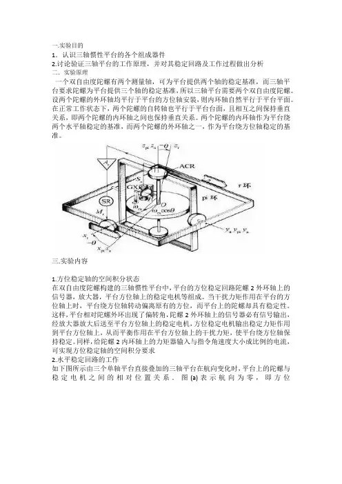
一.实验目的1.认识三轴惯性平台的各个组成器件2.讨论验证三轴平台的工作原理,并对其稳定回路及工作过程做出分析二.实验原理一个双自由度陀螺有两个测量轴,可为平台提供两个轴的稳定基准,而三轴平台要求陀螺为平台提供三个轴的稳定基准,所以三轴平台需要两个双自由度陀螺。
设两个陀螺的外环轴均平行于平台的方位轴安装,则内环轴自然平行于平台平面。
在正常工作状态下,两个陀螺的自转轴也平行于平台台面,且相互之间保持垂直关系,即两个陀螺的内环轴之间也保持垂直关系。
两个陀螺的内环轴作为平台绕两个水平轴稳定的基准,而两个陀螺的外环轴之一,作为平台绕方位轴稳定的基准。
三.实验内容1.方位稳定轴的空间积分状态在双自由度陀螺构建的三轴惯性平台中,平台的方位稳定回路陀螺2外环轴上的信号器,放大器,平台方位轴上的稳定电机等组成。
当干扰力矩作用在平台的方位轴上时,平台绕方位轴转动偏离原有的方位,而平台上的陀螺却具有稳定性。
这样,平台相对陀螺外环出现了偏转角,陀螺2外环轴上的信号器必有信号输出,经放大器放大后送至平台方位轴上的稳定电机,方位稳定电机输出稳定力矩作用到平台方位轴上,从而平衡作用在平台方位轴上的干扰力矩,使平台绕方位轴保持稳定。
同样,给陀螺2内环轴上的力矩器输入与指令角速度大小成比例的电流,可实现方位稳定轴的空间积分要求2.水平稳定回路的工作如下图所示由三个单轴平台直接叠加的三轴平台在航向变化时,平台上的陀螺与稳定电机之间的相对位置关系.图(a)表示航向为零,即方位环环对俯仰环没有转角时陀螺与稳定电机之间的相对位置关系,此时的陀螺Ⅱ感受沿横滚轴(纵向)方向作用到平台上的干扰力矩,信号器输出的信号经横滚放大器A.放大后给横滚轴稳定电机,产生纵向稳定力矩,使平台沿纵向(x.轴)保持稳定,陀螺I感受沿俯仰轴(横向)方向作用到平台上的干扰力矩。
经信号器.放大器和俯仰轴稳定电机,产生沿横向的稳定力矩.使平台沿横向保持稳定。
同样,若给两个陀螺的力矩器输入与指令角速度成比例的电流,平台也可正常工作在空间积分状态。
激光惯导的⼯作原理(⼀)惯性导航体系也称作惯性参考体系,是⼀种不依靠于外部信息、也不向外部辐射能量(如⽆线电导航那样)的⾃主式导航体系。
其作业环境不只包含空中、地上,还可以在⽔下。
惯性导航的根本作业原理是以⽜顿⼒学定律为根底,通过丈量载体在惯性参考系的加速度,将它对时刻进⾏积分,且把它变换到导航坐标系中,就可以得到在导航坐标系中的速度、偏航⾓和⽅位等信息。
惯性导航体系归于推算导航⽅法,即从⼀已知点的⽅位依据接连测得的运动体航向⾓和速度推算出其下⼀点的⽅位,因⽽可接连测出运动体的当前⽅位。
惯性导航体系中的陀螺仪⽤来形成⼀个导航坐标系,使加速度计的丈量轴稳定在该坐标系中,并给出航向和姿势⾓;加速度计⽤来丈量运动体的加速度,通过对时刻的⼀次积分得到速度,速度再通过对时刻的⼀次积分即可得到位移。
现代⽐较常见的⼏种导航技能,包含地理导航、惯性导航、卫星导航、⽆线电导航等等,其中,只要惯性导航是⾃主的,既不向外界辐射东西,也不必看天空中的恒星或接纳外部的信号,它的隐蔽性是最好的。
惯性导航,并不像我们所以为的那样“不靠谱”,像国家的很多战略、战术兵器,再如洲际飞⾏的民航飞机等,都必须依靠惯性导航体系或许惯导体系和其他类型的导航体系的组合。
它的造价也⽐较贵重,像⼀台导航级(即1⼩时差错1海⾥)的惯导体系,⾄少要⼏⼗万,⽽这种精度的导航体系已满⾜装备在波⾳747这样的飞机上了。
现在,跟着mems(微电⼦机械体系)惯性器材技能的前进,商业级、消费等第的惯性导航才逐步⾛进寻常百姓家。
惯性导航体系有如下长处:1、因为它是不依靠于任何外部信息,也不向外部辐射能量的⾃主式体系,故隐蔽性好,也不受外界电磁搅扰的影响;2、可全天候、全时刻地作业于空中、地球表⾯乃⾄⽔下3、能供给⽅位、速度、航向和姿势⾓数据,所发⽣的导航信息接连性好并且噪声低;4、数据更新率⾼、短期精度和稳定性好。
其缺陷是:1、因为导航信息通过积分⽽发⽣,定位差错随时刻⽽增⼤,长期精度差;2、每次使⽤之前需求较长的初始对准时刻;3、设备的价格较贵重;4、不能给出时刻信息。
惯性导航作业一、数据说明:1:惯导系统为指北方位的捷连系统。
初始经度为116.344695283度、纬度为39.975172度,高度h为30米。
初速度v0=[-9.993908270;0.000000000;0.348994967]。
2:jlfw中为600秒的数据,陀螺仪和加速度计采样周期分别为为1/100秒和1/100秒。
3:初始姿态角为[2 1 90](俯仰,横滚,航向,单位为度),jlfw.mat中保存的为比力信息f_INSc(单位m/s^2)、陀螺仪角速率信息wib_INSc(单位rad/s),排列顺序为一~三行分别为X、Y、Z向信息.4: 航向角以逆时针为正。
5:地球椭球长半径re=6378245;地球自转角速度wie=7.292115147e-5;重力加速度g=g0*(1+gk1*c33^2)*(1-2*h/re)/sqrt(1-gk2*c33^2);g0=9.7803267714;gk1=0.00193185138639;gk2=0.00669437999013;c33=sin(lat纬度);二、作业要求:1:可使用MATLAB语言编程,用MATLAB编程时可使用如下形式的语句读取数据:load D:\...文件路径...\jlfw,便可得到比力信息和陀螺仪角速率信息。
用角增量法。
2:(1) 以系统经度为横轴,纬度为纵轴(单位均要转换为:度)做出系统位置曲线图;(2) 做出系统东向速度和北向速度随时间变化曲线图(速度单位:m/s,时间单位:s);(3) 分别做出系统姿态角随时间变化曲线图(俯仰,横滚,航向,单位转换为:度,时间单位:s);以上结果均要附在作业报告中。
3:在作业报告中要写出“程序流程图、现阶段学习小结”,写明联系方式。
(注意程序流程图不是课本上的惯导解算流程,而是你程序分为哪几个模块、是怎样一步步执行的,什么位置循环等,让别人根据该流程图能够编出相应程序) (学习小结按条写,不用写套话) 4:作业以纸质报告形式提交,附源程序。
山东科技大学2007—2008学年第二学期
《陀螺仪与惯性导航》考试试卷(卷)
班级姓名学号
一、填空题(每题5分,共40分)
1.工程上,为了使陀螺转子获得三个所需要的角转动自由度,典型的办法是将陀螺转子支
撑在由构成的卡登万向环架中,并确保转子与支承点重合,所以转子可看作。
2.陀螺运动的基本特性有,和。
3.捷联式惯导系统的姿态算法有、和。
4.在绘制一幅地图时,必须规定以作为
计算和表达的基准。
我们把称为基准比例尺。
海图的比例尺越小,同样面积的一幅海图,所包含的海区范围就越,标绘的图形越。
5.根据加速度测量相对的坐标系不同,及加速度计是否放在平台上,惯性导航系统可以分
为、和。
6.常值陀螺漂移引起惯性导航系统的稳态误差有、、。
7.舒拉条件,舒拉角频率,舒拉振荡周期。
8.经典导航系统有、、、、。
二、简答题(每题10分,共40分)
1.试述卡尔曼滤波的实质。
2. 试比较GPS 和INS 优缺点。
3. 简述光线陀螺仪的工作原理。
4. 试比较平台式与捷联式导航系统。
三、计算题(每题10分,共20分)
1. 设陀螺仪转子的极转动惯量2398z I =⋅克厘米,转子的转速为24000n =转/分钟,求转子
的角动量。
2. 简述哥氏定理,并说明结果中各项含义。
惯性导航原理实验课程设计一、课程目标知识目标:1. 学生能够理解惯性导航系统的基本原理,掌握其工作方式和组成结构。
2. 学生能够掌握惯性导航系统中的关键参数,如加速度、角速度等,并了解它们对导航精度的影响。
3. 学生能够描述惯性导航系统在不同环境下的误差来源及其补偿方法。
技能目标:1. 学生能够操作惯性导航实验设备,进行数据采集、处理和分析。
2. 学生能够利用实验数据,结合理论知识,完成简单的惯性导航路径推算。
3. 学生能够通过实验,培养实际操作能力和团队合作能力。
情感态度价值观目标:1. 学生能够培养对惯性导航技术的好奇心与探索精神,提高对物理学科的兴趣。
2. 学生能够认识到惯性导航技术在现实生活中的应用,增强科技改变生活的意识。
3. 学生能够通过课程学习,树立正确的科学态度,培养严谨、务实的作风。
课程性质分析:本课程为物理学科实验课程,以惯性导航原理为教学内容,结合实际操作,提高学生的实践能力。
学生特点分析:学生为高中二年级学生,已具备一定的物理知识和实验操作能力,对高新技术具有较强的好奇心。
教学要求:课程设计应注重理论与实践相结合,强调学生的动手能力,将抽象的物理原理具体化,提高学生的学习兴趣和实际应用能力。
通过课程目标的分解,使学生在学习过程中达到预期的学习成果,为后续教学设计和评估提供依据。
二、教学内容1. 理论知识:- 惯性导航系统原理:包括牛顿运动定律、惯性参考系等基本概念。
- 惯性导航系统组成:陀螺仪、加速度计、计算机及软件等。
- 惯性导航系统误差分析:系统误差、随机误差、环境因素等影响。
- 误差补偿方法:系统标定、卡尔曼滤波等。
2. 实践操作:- 惯性导航设备认识:了解设备结构、功能及操作方法。
- 数据采集与处理:学习如何采集加速度、角速度等数据,并进行处理分析。
- 惯性导航路径推算:利用采集到的数据,结合理论知识,进行路径推算。
3. 教学大纲安排:- 第一课时:惯性导航系统原理及组成介绍。
导航原理作业(惯性导航部分)1.题目内容(即本页)2.程序设计说明及代码3.计算或仿真结果及分析4.仿真中遇到的问题或体会一枚导弹采用捷联惯性导航系统,三个速率陀螺仪Gx, Gy, Gz 和三个加速度计Ax, Ay, Az 的敏感轴分别沿着着弹体坐标系的Xb, Yb, Zb轴。
初始时刻该导弹处在北纬45.75度,东经126.63度。
第一种情形:正对导弹进行地面静态测试(导弹质心相对地面静止)。
初始时刻弹体坐标系和地理坐标系重合,如图所示,弹体的Xb轴指东,Yb轴指北,Zb轴指天。
此后弹体坐标系Xb-Yb-Zb 相对地理坐标系的转动如下:首先,弹体绕Zb(方位轴)转过-10 度;接着,弹体绕Xb(俯仰轴)转过15 度;然后,弹体绕Yb(滚动轴)转过20 度;最后弹体相对地面停止旋转。
请分别用方向余弦矩阵和四元数两种方法计算:弹体经过三次旋转并停止之后,弹体上三个加速度计Ax, Ay, Az的输出。
取重力加速度的大小g = 9.8m/s2。
第二种情形:导弹正在飞行中。
初始时刻弹体坐标系仍和地理坐标系重合;且导弹初始高度200m,初始北向速度1800 m/s,初始东向速度和垂直速度都为零。
陀螺仪和加速度计的输出都为脉冲数形式,陀螺输出的每个脉冲代表0.00001弧度的角增量。
加速度计输出的每个脉冲代表1μg,1g = 9.8m/s2。
陀螺仪和加速度计输出的采样频率都为10Hz,在200秒内三个陀螺仪和三个加速度计的输出存在了数据文件gaout.mat中,内含一矩阵变量ga,有2000行,6列。
每一行中的数据代表每个采样时刻三个陀螺Gx, Gy, Gz和三个加速度计Ax, Ay, Az将地球视为理想的球体,半径6371.00公里,且不考虑仪表误差,也不考虑弹体高度对重力加速度的影响。
选取弹体的姿态计算周期为0.1秒,速度和位置的计算周期为1秒。
(1)请计算200秒后弹体到达的经纬度和高度,东向和北向速度;(2)请计算200秒后弹体相对当地地理坐标系的姿态四元数;(3)请绘制出200秒内导弹的经、纬度变化曲线(以经度为横轴,纬度为纵轴);(4)请绘制出200秒内导弹的高度变化曲线(以时间为横轴,高度为纵轴)。
惯性导航技术用于既有线升级改造施工工法惯性导航技术用于既有线升级改造施工工法一、前言随着社会的发展和城市规模的扩大,既有线的升级改造成为了一个重要的工程项目。
而在升级改造的过程中,如何准确高效地进行线路施工成为了一个关键的问题。
惯性导航技术作为一种先进的定位导航技术,为既有线升级改造施工工法提供了新的解决方案。
本文将对该工法的工法特点、适应范围、工艺原理、施工工艺、劳动组织、机具设备、质量控制、安全措施、经济技术分析以及工程实例进行详细介绍。
二、工法特点惯性导航技术用于既有线升级改造施工工法具有以下几个特点:1. 高精度定位:通过惯性导航技术,可以实现高精度的线路定位,保证施工精度和效率;2. 独立系统:该工法独立于GPS等外部定位系统,具有自主性和独立性,不受信号干扰;3. 实时更新:惯性导航技术能够实时更新线路的位置和状态信息,为施工提供了准确的参考依据;4. 适应性强:该工法适应范围广,可用于城市地下管网、电力线路、铁路线路等各种既有线的升级改造施工。
三、适应范围惯性导航技术用于既有线升级改造施工工法适用于各类既有线的升级改造,包括但不限于以下领域:1.地下管网:如城市供水管道、排水管道、天然气管道等;2.电力线路:如电缆线路、输电线路等;3. 铁路线路:如轨道、信号线等;4. 通信线路:如光纤线路、电信线路等。
四、工艺原理对施工工法与实际工程之间的联系、采取的技术措施进行具体的分析和解释,让读者了解该工法的理论依据和实际应用。
惯性导航技术基于惯性测量单元(IMU)和全球卫星定位系统(GNSS)等技术,通过收集和处理线路的位置、方向、速度等信息,实现对线路的实时跟踪和定位。
五、施工工艺对施工工法的各个施工阶段进行详细的描述,让读者了解施工过程中的每一个细节。
施工工艺包括以下几个步骤:1. 前期准备:确定施工范围和工期,进行必要的勘察和测量工作;2. 设计方案:根据升级改造的要求,制定合理的设计方案;3. 设备准备:选取适合的惯性导航设备和相关工具;4. 施工施工:根据设计方案,进行线路的改造和修复;5. 质量验收:对施工成果进行质量验收,确保达到设计要求。
惯性导航系统的基本原理、特点及在现代生活中的应用
惯性导航系统的基本原理
惯性导航系统也称作惯性参考系统,是一种不依赖于外部信息、也不向外部辐射能量(如无线电导航那样)的自主式导航系统。
其工作环境不仅包括空中、地面,还可以在水下。
惯性导航的基本工作原理是以牛顿力学定律为基础,通过测量载体在惯性参考系的加速度,将它对时间进行积分,且把它变换到导航坐标系中,就能够得到在导航坐标系中的速度、偏航角和位置等信息。
惯性导航系统属于推算导航方式,即从一已知点的位置根据连续测得的运动体航向角和速度推算出其下一点的位置,因而可连续测出运动体的当前位置。
惯性导航系统中的陀螺仪用来形成一个导航坐标系,使加速度计的测量轴稳定在该坐标系中,并给出航向和姿态角;加速度计用来测量运动体的加速度,经过对时间的一次积分得到速度,速度再经过对时间的一次积分即可得到距离。
惯性导航技术的理论基础是牛顿力学基本定律。
惯性导航系统是以陀螺和加速度计为敏感器件的导航参数解算系统,该系统根据陀螺的输出建立导航坐标系,根据加速度计输出解算出运载体在导航坐标系中的速度和位置。
惯性导航系统分成平台式惯性导航系统和捷联式惯性导航系统两大类。
平台式惯性导航系统将惯性测量元件安装在惯性平台上,惯性平台稳定在预定的坐标系内,为加速度计提供一个测量基准,并使惯性测量元件体角运动的影响。
导航计算机根据加速度计的输出和初始条件进行导航解算,得出载的位置、速度等导航参数。
捷联式惯性导航系统将惯性测量元件直接固联在载体上,测量沿载体坐标系的角速度和角加速度,计算机则利用陀螺的输出,进行坐标变换,求解载体的即时速度、位置等导航参数。
惯性导航仅依靠惯性装置本身就能在载体内部独立地完成导航任务,不需要与外界发生任何信号联系,具有高度的自主性。
这在战略和战术应用上具有重要的意义。
但惯性导航的定位误差会随时间逐步增加,必须不断地进行误差修正,才能保证达到要求的精度。
陀螺仪
陀螺仪通常是指安装在万向支架中高度旋转的转子,转子同时可绕垂直于自转轴的一根轴或两根轴进动,前者称单自由度陀螺仪,后者称二自由度陀螺仪。
陀螺仪具有定轴性和进动性,利用这些特性制成了敏感角速度的速率陀螺和敏感角偏差的位置陀螺。
对于光学、MEMS等技术被进入于陀螺仪的研制,现在习惯上把能够完成陀螺功能的装置统称为陀螺。
陀螺仪的种类很多,按用途来分,它可以分为传感陀螺仪和指示陀螺仪。
传感陀螺仪用于飞行体运动的自动控制系统中,作为水平、垂直、俯仰、航向和角速度传感器。
指示陀螺仪主要用于飞行状态的指示,作为驾驶和领航仪表使用。
陀螺仪分为,压电陀螺仪,微机械陀螺仪,光纤陀螺仪和激光陀螺仪,它们都是电子式的,并且它们可以和加速度计,磁阻芯片,GPS,做成惯性导航控制系统。
加速度计
加速度是用来计测量加速度的仪表。
它通过测量组件在某个轴向的受力情况来得到结果,表现形式为轴向的加速度大小和方向,但用来测量设备相对地面的摆放姿势的精确度不高,该缺陷可以通过陀螺仪得到补偿。
惯性导航的特点:
惯性导航系统有如下优点:1、由于它是不依赖于任何外部信息,也不向外部辐射能量的自主式系统,故隐蔽性好,也不受外界电磁干扰的影响;2、可全天候、全时间地工作于空中、地球表面乃至水下;3、能提供位置、速度、航向和姿态角数据,所产生的导航信息连续性好而且噪声低;4、数据更新率高、短期精度和稳定性好。
其缺点是:1、由于导航信息经过积分而产生,定位误差随时间而增大,长期精度差;2、每次使用之前需要较长的初始对准时间;3、设备的价格较昂贵;4、不能给出时间信息。
但惯导有固定的漂移率,这样会造成物体运动的误差,因此射程远的武器通常会采用指令、GPS等对惯导进行定时修正,以获取持续准确的位置参数。
惯导系统目前已经发展出挠性惯导、光纤惯导、激光惯导、微固态惯性仪表等多种方式。
陀螺仪由传统的绕线陀螺发展到静电陀螺、激光陀螺、光纤陀螺、微机械陀螺等。
激光陀螺测量动态范围宽,线性度好,性能稳定,具有良好的温度稳定性和重复性,在高精度的应用领域中一直占据着主导位置。
由于科技进步,成本较低的光纤陀螺(FOG)和微机械陀螺(MEMS)精度越来越高,是未来陀螺技术发展的方向。
惯性导航系统在现代生活中的应用
现代生活中惯性导航系统已经涉及到我们的生活中的很多发面,在陆地车辆、船舶、舰艇、航天飞行器、大地测量、资源勘测、海洋探测、铁路、航天飞机及执导武器方面,尤其是在军事方面得到了大量的应用,战斗机、坦克、导弹都用到了惯性导航技术。
随着惯性导航技术的发展与成熟,人们的出行、娱乐都会涉及到惯性导航。
手机、摄像机、玩具、航模和现在很火热的VR都已经运用到了惯性导航技术。
现在的GPS就是惯性导航系统在生活中应用最成功的例子。
在未来的生活中惯性导航会涉及到更多的方面,对我们的生活产生更大的帮助。