深度学习综述讨论简介deepLearning
- 格式:pptx
- 大小:5.91 MB
- 文档页数:51
Deeplearning4j的分布式深度学习深度学习已经成为了人工智能领域的热门话题,而Deeplearning4j作为一种分布式深度学习框架,正受到越来越多的关注。
本文将介绍Deeplearning4j的分布式深度学习相关概念、特点以及其在各个领域的应用。
一、什么是分布式深度学习分布式深度学习是指将深度学习的计算任务分配到多个计算节点上进行并行计算的一种方式。
传统的深度学习方法通常在单个计算节点上进行运算,而分布式深度学习则实现了多个计算节点之间的数据共享与通信,从而提升了计算效率和模型的训练速度。
二、Deeplearning4j框架简介Deeplearning4j是一种基于Java语言开发的分布式深度学习框架,其具有以下特点:1. 可扩展性:Deeplearning4j支持在多台计算节点上进行并行计算,可轻松地扩展到大规模的数据和计算资源。
2. 多样化的模型支持:Deeplearning4j支持各种网络模型的构建,包括卷积神经网络、循环神经网络以及深度信念网络等。
3. 高性能的计算能力:Deeplearning4j通过优化算法和并行计算,提供了高效的深度学习计算能力。
4. 灵活的数据处理:Deeplearning4j支持常见的数据预处理操作,并提供了灵活的数据流水线功能。
5. 丰富的工具生态系统:Deeplearning4j提供了多种工具和库,如ND4J、DataVec等,用于支持数据处理、模型构建和模型评估等环节。
三、Deeplearning4j的应用领域Deeplearning4j作为一种分布式深度学习框架,广泛应用于各个领域,包括但不限于以下几个方面:1. 计算机视觉:Deeplearning4j在计算机视觉领域的应用非常广泛,包括图像分类、目标检测、图像生成等。
通过分布式计算技术,可以大幅提升图像处理任务的效率,并提升模型的准确性。
2. 语音识别:Deeplearning4j在语音识别领域具有出色的表现。

国外近十年深度学习实证研究综述主题、情境、方法及结果一、概述:二、主题分类:计算机视觉:该主题主要关注图像识别、目标检测、图像生成等任务。
研究者利用深度学习模型,如卷积神经网络(CNN),在图像分类、人脸识别、物体检测等任务上取得了显著成果。
自然语言处理:自然语言处理是深度学习的另一重要应用领域。
研究者使用循环神经网络(RNN)、长短期记忆网络(LSTM)、变压器(Transformer)等模型进行文本生成、情感分析、机器翻译等任务,推动了自然语言处理技术的发展。
语音识别与生成:深度学习在语音识别和语音合成方面也有广泛应用。
研究者利用深度学习模型进行语音特征提取、语音识别和语音合成,提高了语音技术的准确性和自然度。
游戏与人工智能:深度学习在游戏领域的应用也日益增多。
研究者利用深度学习模型进行游戏策略学习、游戏内容生成等任务,提高了游戏的智能性和趣味性。
医疗与健康:深度学习在医疗领域的应用也备受关注。
研究者利用深度学习模型进行疾病诊断、药物研发、医疗影像分析等任务,为医疗健康领域的发展提供了有力支持。
这些主题分类展示了深度学习在不同领域和应用场景中的广泛应用和巨大潜力。
通过对这些主题的深入研究和分析,我们可以更好地理解深度学习的发展趋势和应用前景。
1. 计算机视觉在计算机视觉领域,深度学习技术的应用已经取得了显著的突破。
近年来,卷积神经网络(CNN)成为了该领域的主导模型,特别是在图像分类、目标检测、图像分割等方面。
AlexNet、VGG、GoogleNet、ResNet等模型的出现,不断刷新了图像分类任务上的准确率记录。
主题:计算机视觉的核心任务是让机器能够像人一样“看懂”图像和视频,从而进行自动分析和理解。
深度学习通过模拟人脑神经元的连接方式,构建出复杂的网络结构,实现对图像的高效特征提取和分类。
情境:计算机视觉的应用场景非常广泛,包括人脸识别、自动驾驶、医学影像分析、安全监控等。
在这些场景中,深度学习模型需要处理的数据集往往规模庞大,且存在噪声、模糊等问题,因此模型的鲁棒性和泛化能力成为研究重点。
deeplearning tutorial (2) 原理简介+代码详解【原创实用版】目录一、Deep Learning 简介二、Deep Learning 原理1.神经网络2.梯度下降3.反向传播三、Deep Learning 模型1.卷积神经网络(CNN)2.循环神经网络(RNN)3.生成对抗网络(GAN)四、Deep Learning 应用实例五、Deep Learning 代码详解1.TensorFlow 安装与使用2.神经网络构建与训练3.卷积神经网络(CNN)实例4.循环神经网络(RNN)实例5.生成对抗网络(GAN)实例正文一、Deep Learning 简介Deep Learning 是一种机器学习方法,其主要目标是让计算机模仿人脑的工作方式,通过多层次的抽象表示来理解和处理复杂的数据。
Deep Learning 在图像识别、语音识别、自然语言处理等领域取得了显著的成果,成为当前人工智能领域的研究热点。
二、Deep Learning 原理1.神经网络神经网络是 Deep Learning 的基本构成单元,它由多个神经元组成,每个神经元接收一组输入信号,根据权重和偏置计算输出信号,并将输出信号传递给其他神经元。
神经网络通过不断调整权重和偏置,使得模型能够逐渐逼近目标函数。
2.梯度下降梯度下降是一种优化算法,用于求解神经网络的权重和偏置。
梯度下降算法通过计算目标函数关于权重和偏置的梯度,不断更新权重和偏置,使得模型的预测误差逐渐减小。
3.反向传播反向传播是神经网络中计算梯度的一种方法。
在训练过程中,神经网络根据实际输出和预期输出的误差,按照梯度下降算法计算梯度,然后沿着梯度反向更新权重和偏置,使得模型的预测误差逐渐减小。
三、Deep Learning 模型1.卷积神经网络(CNN)卷积神经网络是一种特殊的神经网络,广泛应用于图像识别领域。
CNN 通过卷积层、池化层和全连接层等操作,对图像进行特征提取和分类,取得了在图像识别领域的突破性成果。
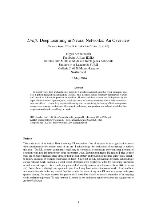
Draft:Deep Learning in Neural Networks:An OverviewTechnical Report IDSIA-03-14/arXiv:1404.7828(v1.5)[cs.NE]J¨u rgen SchmidhuberThe Swiss AI Lab IDSIAIstituto Dalle Molle di Studi sull’Intelligenza ArtificialeUniversity of Lugano&SUPSIGalleria2,6928Manno-LuganoSwitzerland15May2014AbstractIn recent years,deep artificial neural networks(including recurrent ones)have won numerous con-tests in pattern recognition and machine learning.This historical survey compactly summarises relevantwork,much of it from the previous millennium.Shallow and deep learners are distinguished by thedepth of their credit assignment paths,which are chains of possibly learnable,causal links between ac-tions and effects.I review deep supervised learning(also recapitulating the history of backpropagation),unsupervised learning,reinforcement learning&evolutionary computation,and indirect search for shortprograms encoding deep and large networks.PDF of earlier draft(v1):http://www.idsia.ch/∼juergen/DeepLearning30April2014.pdfLATEX source:http://www.idsia.ch/∼juergen/DeepLearning30April2014.texComplete BIBTEXfile:http://www.idsia.ch/∼juergen/bib.bibPrefaceThis is the draft of an invited Deep Learning(DL)overview.One of its goals is to assign credit to those who contributed to the present state of the art.I acknowledge the limitations of attempting to achieve this goal.The DL research community itself may be viewed as a continually evolving,deep network of scientists who have influenced each other in complex ways.Starting from recent DL results,I tried to trace back the origins of relevant ideas through the past half century and beyond,sometimes using“local search”to follow citations of citations backwards in time.Since not all DL publications properly acknowledge earlier relevant work,additional global search strategies were employed,aided by consulting numerous neural network experts.As a result,the present draft mostly consists of references(about800entries so far).Nevertheless,through an expert selection bias I may have missed important work.A related bias was surely introduced by my special familiarity with the work of my own DL research group in the past quarter-century.For these reasons,the present draft should be viewed as merely a snapshot of an ongoing credit assignment process.To help improve it,please do not hesitate to send corrections and suggestions to juergen@idsia.ch.Contents1Introduction to Deep Learning(DL)in Neural Networks(NNs)3 2Event-Oriented Notation for Activation Spreading in FNNs/RNNs3 3Depth of Credit Assignment Paths(CAPs)and of Problems4 4Recurring Themes of Deep Learning54.1Dynamic Programming(DP)for DL (5)4.2Unsupervised Learning(UL)Facilitating Supervised Learning(SL)and RL (6)4.3Occam’s Razor:Compression and Minimum Description Length(MDL) (6)4.4Learning Hierarchical Representations Through Deep SL,UL,RL (6)4.5Fast Graphics Processing Units(GPUs)for DL in NNs (6)5Supervised NNs,Some Helped by Unsupervised NNs75.11940s and Earlier (7)5.2Around1960:More Neurobiological Inspiration for DL (7)5.31965:Deep Networks Based on the Group Method of Data Handling(GMDH) (8)5.41979:Convolution+Weight Replication+Winner-Take-All(WTA) (8)5.51960-1981and Beyond:Development of Backpropagation(BP)for NNs (8)5.5.1BP for Weight-Sharing Feedforward NNs(FNNs)and Recurrent NNs(RNNs)..95.6Late1980s-2000:Numerous Improvements of NNs (9)5.6.1Ideas for Dealing with Long Time Lags and Deep CAPs (10)5.6.2Better BP Through Advanced Gradient Descent (10)5.6.3Discovering Low-Complexity,Problem-Solving NNs (11)5.6.4Potential Benefits of UL for SL (11)5.71987:UL Through Autoencoder(AE)Hierarchies (12)5.81989:BP for Convolutional NNs(CNNs) (13)5.91991:Fundamental Deep Learning Problem of Gradient Descent (13)5.101991:UL-Based History Compression Through a Deep Hierarchy of RNNs (14)5.111992:Max-Pooling(MP):Towards MPCNNs (14)5.121994:Contest-Winning Not So Deep NNs (15)5.131995:Supervised Recurrent Very Deep Learner(LSTM RNN) (15)5.142003:More Contest-Winning/Record-Setting,Often Not So Deep NNs (16)5.152006/7:Deep Belief Networks(DBNs)&AE Stacks Fine-Tuned by BP (17)5.162006/7:Improved CNNs/GPU-CNNs/BP-Trained MPCNNs (17)5.172009:First Official Competitions Won by RNNs,and with MPCNNs (18)5.182010:Plain Backprop(+Distortions)on GPU Yields Excellent Results (18)5.192011:MPCNNs on GPU Achieve Superhuman Vision Performance (18)5.202011:Hessian-Free Optimization for RNNs (19)5.212012:First Contests Won on ImageNet&Object Detection&Segmentation (19)5.222013-:More Contests and Benchmark Records (20)5.22.1Currently Successful Supervised Techniques:LSTM RNNs/GPU-MPCNNs (21)5.23Recent Tricks for Improving SL Deep NNs(Compare Sec.5.6.2,5.6.3) (21)5.24Consequences for Neuroscience (22)5.25DL with Spiking Neurons? (22)6DL in FNNs and RNNs for Reinforcement Learning(RL)236.1RL Through NN World Models Yields RNNs With Deep CAPs (23)6.2Deep FNNs for Traditional RL and Markov Decision Processes(MDPs) (24)6.3Deep RL RNNs for Partially Observable MDPs(POMDPs) (24)6.4RL Facilitated by Deep UL in FNNs and RNNs (25)6.5Deep Hierarchical RL(HRL)and Subgoal Learning with FNNs and RNNs (25)6.6Deep RL by Direct NN Search/Policy Gradients/Evolution (25)6.7Deep RL by Indirect Policy Search/Compressed NN Search (26)6.8Universal RL (27)7Conclusion271Introduction to Deep Learning(DL)in Neural Networks(NNs) Which modifiable components of a learning system are responsible for its success or failure?What changes to them improve performance?This has been called the fundamental credit assignment problem(Minsky, 1963).There are general credit assignment methods for universal problem solvers that are time-optimal in various theoretical senses(Sec.6.8).The present survey,however,will focus on the narrower,but now commercially important,subfield of Deep Learning(DL)in Artificial Neural Networks(NNs).We are interested in accurate credit assignment across possibly many,often nonlinear,computational stages of NNs.Shallow NN-like models have been around for many decades if not centuries(Sec.5.1).Models with several successive nonlinear layers of neurons date back at least to the1960s(Sec.5.3)and1970s(Sec.5.5). An efficient gradient descent method for teacher-based Supervised Learning(SL)in discrete,differentiable networks of arbitrary depth called backpropagation(BP)was developed in the1960s and1970s,and ap-plied to NNs in1981(Sec.5.5).BP-based training of deep NNs with many layers,however,had been found to be difficult in practice by the late1980s(Sec.5.6),and had become an explicit research subject by the early1990s(Sec.5.9).DL became practically feasible to some extent through the help of Unsupervised Learning(UL)(e.g.,Sec.5.10,5.15).The1990s and2000s also saw many improvements of purely super-vised DL(Sec.5).In the new millennium,deep NNs havefinally attracted wide-spread attention,mainly by outperforming alternative machine learning methods such as kernel machines(Vapnik,1995;Sch¨o lkopf et al.,1998)in numerous important applications.In fact,supervised deep NNs have won numerous of-ficial international pattern recognition competitions(e.g.,Sec.5.17,5.19,5.21,5.22),achieving thefirst superhuman visual pattern recognition results in limited domains(Sec.5.19).Deep NNs also have become relevant for the more generalfield of Reinforcement Learning(RL)where there is no supervising teacher (Sec.6).Both feedforward(acyclic)NNs(FNNs)and recurrent(cyclic)NNs(RNNs)have won contests(Sec.5.12,5.14,5.17,5.19,5.21,5.22).In a sense,RNNs are the deepest of all NNs(Sec.3)—they are general computers more powerful than FNNs,and can in principle create and process memories of ar-bitrary sequences of input patterns(e.g.,Siegelmann and Sontag,1991;Schmidhuber,1990a).Unlike traditional methods for automatic sequential program synthesis(e.g.,Waldinger and Lee,1969;Balzer, 1985;Soloway,1986;Deville and Lau,1994),RNNs can learn programs that mix sequential and parallel information processing in a natural and efficient way,exploiting the massive parallelism viewed as crucial for sustaining the rapid decline of computation cost observed over the past75years.The rest of this paper is structured as follows.Sec.2introduces a compact,event-oriented notation that is simple yet general enough to accommodate both FNNs and RNNs.Sec.3introduces the concept of Credit Assignment Paths(CAPs)to measure whether learning in a given NN application is of the deep or shallow type.Sec.4lists recurring themes of DL in SL,UL,and RL.Sec.5focuses on SL and UL,and on how UL can facilitate SL,although pure SL has become dominant in recent competitions(Sec.5.17-5.22). Sec.5is arranged in a historical timeline format with subsections on important inspirations and technical contributions.Sec.6on deep RL discusses traditional Dynamic Programming(DP)-based RL combined with gradient-based search techniques for SL or UL in deep NNs,as well as general methods for direct and indirect search in the weight space of deep FNNs and RNNs,including successful policy gradient and evolutionary methods.2Event-Oriented Notation for Activation Spreading in FNNs/RNNs Throughout this paper,let i,j,k,t,p,q,r denote positive integer variables assuming ranges implicit in the given contexts.Let n,m,T denote positive integer constants.An NN’s topology may change over time(e.g.,Fahlman,1991;Ring,1991;Weng et al.,1992;Fritzke, 1994).At any given moment,it can be described as afinite subset of units(or nodes or neurons)N= {u1,u2,...,}and afinite set H⊆N×N of directed edges or connections between nodes.FNNs are acyclic graphs,RNNs cyclic.Thefirst(input)layer is the set of input units,a subset of N.In FNNs,the k-th layer(k>1)is the set of all nodes u∈N such that there is an edge path of length k−1(but no longer path)between some input unit and u.There may be shortcut connections between distant layers.The NN’s behavior or program is determined by a set of real-valued,possibly modifiable,parameters or weights w i(i=1,...,n).We now focus on a singlefinite episode or epoch of information processing and activation spreading,without learning through weight changes.The following slightly unconventional notation is designed to compactly describe what is happening during the runtime of the system.During an episode,there is a partially causal sequence x t(t=1,...,T)of real values that I call events.Each x t is either an input set by the environment,or the activation of a unit that may directly depend on other x k(k<t)through a current NN topology-dependent set in t of indices k representing incoming causal connections or links.Let the function v encode topology information and map such event index pairs(k,t)to weight indices.For example,in the non-input case we may have x t=f t(net t)with real-valued net t= k∈in t x k w v(k,t)(additive case)or net t= k∈in t x k w v(k,t)(multiplicative case), where f t is a typically nonlinear real-valued activation function such as tanh.In many recent competition-winning NNs(Sec.5.19,5.21,5.22)there also are events of the type x t=max k∈int (x k);some networktypes may also use complex polynomial activation functions(Sec.5.3).x t may directly affect certain x k(k>t)through outgoing connections or links represented through a current set out t of indices k with t∈in k.Some non-input events are called output events.Note that many of the x t may refer to different,time-varying activations of the same unit in sequence-processing RNNs(e.g.,Williams,1989,“unfolding in time”),or also in FNNs sequentially exposed to time-varying input patterns of a large training set encoded as input events.During an episode,the same weight may get reused over and over again in topology-dependent ways,e.g.,in RNNs,or in convolutional NNs(Sec.5.4,5.8).I call this weight sharing across space and/or time.Weight sharing may greatly reduce the NN’s descriptive complexity,which is the number of bits of information required to describe the NN (Sec.4.3).In Supervised Learning(SL),certain NN output events x t may be associated with teacher-given,real-valued labels or targets d t yielding errors e t,e.g.,e t=1/2(x t−d t)2.A typical goal of supervised NN training is tofind weights that yield episodes with small total error E,the sum of all such e t.The hope is that the NN will generalize well in later episodes,causing only small errors on previously unseen sequences of input events.Many alternative error functions for SL and UL are possible.SL assumes that input events are independent of earlier output events(which may affect the environ-ment through actions causing subsequent perceptions).This assumption does not hold in the broaderfields of Sequential Decision Making and Reinforcement Learning(RL)(Kaelbling et al.,1996;Sutton and Barto, 1998;Hutter,2005)(Sec.6).In RL,some of the input events may encode real-valued reward signals given by the environment,and a typical goal is tofind weights that yield episodes with a high sum of reward signals,through sequences of appropriate output actions.Sec.5.5will use the notation above to compactly describe a central algorithm of DL,namely,back-propagation(BP)for supervised weight-sharing FNNs and RNNs.(FNNs may be viewed as RNNs with certainfixed zero weights.)Sec.6will address the more general RL case.3Depth of Credit Assignment Paths(CAPs)and of ProblemsTo measure whether credit assignment in a given NN application is of the deep or shallow type,I introduce the concept of Credit Assignment Paths or CAPs,which are chains of possibly causal links between events.Let usfirst focus on SL.Consider two events x p and x q(1≤p<q≤T).Depending on the appli-cation,they may have a Potential Direct Causal Connection(PDCC)expressed by the Boolean predicate pdcc(p,q),which is true if and only if p∈in q.Then the2-element list(p,q)is defined to be a CAP from p to q(a minimal one).A learning algorithm may be allowed to change w v(p,q)to improve performance in future episodes.More general,possibly indirect,Potential Causal Connections(PCC)are expressed by the recursively defined Boolean predicate pcc(p,q),which in the SL case is true only if pdcc(p,q),or if pcc(p,k)for some k and pdcc(k,q).In the latter case,appending q to any CAP from p to k yields a CAP from p to q(this is a recursive definition,too).The set of such CAPs may be large but isfinite.Note that the same weight may affect many different PDCCs between successive events listed by a given CAP,e.g.,in the case of RNNs, or weight-sharing FNNs.Suppose a CAP has the form(...,k,t,...,q),where k and t(possibly t=q)are thefirst successive elements with modifiable w v(k,t).Then the length of the suffix list(t,...,q)is called the CAP’s depth (which is0if there are no modifiable links at all).This depth limits how far backwards credit assignment can move down the causal chain tofind a modifiable weight.1Suppose an episode and its event sequence x1,...,x T satisfy a computable criterion used to decide whether a given problem has been solved(e.g.,total error E below some threshold).Then the set of used weights is called a solution to the problem,and the depth of the deepest CAP within the sequence is called the solution’s depth.There may be other solutions(yielding different event sequences)with different depths.Given somefixed NN topology,the smallest depth of any solution is called the problem’s depth.Sometimes we also speak of the depth of an architecture:SL FNNs withfixed topology imply a problem-independent maximal problem depth bounded by the number of non-input layers.Certain SL RNNs withfixed weights for all connections except those to output units(Jaeger,2001;Maass et al.,2002; Jaeger,2004;Schrauwen et al.,2007)have a maximal problem depth of1,because only thefinal links in the corresponding CAPs are modifiable.In general,however,RNNs may learn to solve problems of potentially unlimited depth.Note that the definitions above are solely based on the depths of causal chains,and agnostic of the temporal distance between events.For example,shallow FNNs perceiving large“time windows”of in-put events may correctly classify long input sequences through appropriate output events,and thus solve shallow problems involving long time lags between relevant events.At which problem depth does Shallow Learning end,and Deep Learning begin?Discussions with DL experts have not yet yielded a conclusive response to this question.Instead of committing myself to a precise answer,let me just define for the purposes of this overview:problems of depth>10require Very Deep Learning.The difficulty of a problem may have little to do with its depth.Some NNs can quickly learn to solve certain deep problems,e.g.,through random weight guessing(Sec.5.9)or other types of direct search (Sec.6.6)or indirect search(Sec.6.7)in weight space,or through training an NNfirst on shallow problems whose solutions may then generalize to deep problems,or through collapsing sequences of(non)linear operations into a single(non)linear operation—but see an analysis of non-trivial aspects of deep linear networks(Baldi and Hornik,1994,Section B).In general,however,finding an NN that precisely models a given training set is an NP-complete problem(Judd,1990;Blum and Rivest,1992),also in the case of deep NNs(S´ıma,1994;de Souto et al.,1999;Windisch,2005);compare a survey of negative results(S´ıma, 2002,Section1).Above we have focused on SL.In the more general case of RL in unknown environments,pcc(p,q) is also true if x p is an output event and x q any later input event—any action may affect the environment and thus any later perception.(In the real world,the environment may even influence non-input events computed on a physical hardware entangled with the entire universe,but this is ignored here.)It is possible to model and replace such unmodifiable environmental PCCs through a part of the NN that has already learned to predict(through some of its units)input events(including reward signals)from former input events and actions(Sec.6.1).Its weights are frozen,but can help to assign credit to other,still modifiable weights used to compute actions(Sec.6.1).This approach may lead to very deep CAPs though.Some DL research is about automatically rephrasing problems such that their depth is reduced(Sec.4). In particular,sometimes UL is used to make SL problems less deep,e.g.,Sec.5.10.Often Dynamic Programming(Sec.4.1)is used to facilitate certain traditional RL problems,e.g.,Sec.6.2.Sec.5focuses on CAPs for SL,Sec.6on the more complex case of RL.4Recurring Themes of Deep Learning4.1Dynamic Programming(DP)for DLOne recurring theme of DL is Dynamic Programming(DP)(Bellman,1957),which can help to facili-tate credit assignment under certain assumptions.For example,in SL NNs,backpropagation itself can 1An alternative would be to count only modifiable links when measuring depth.In many typical NN applications this would not make a difference,but in some it would,e.g.,Sec.6.1.be viewed as a DP-derived method(Sec.5.5).In traditional RL based on strong Markovian assumptions, DP-derived methods can help to greatly reduce problem depth(Sec.6.2).DP algorithms are also essen-tial for systems that combine concepts of NNs and graphical models,such as Hidden Markov Models (HMMs)(Stratonovich,1960;Baum and Petrie,1966)and Expectation Maximization(EM)(Dempster et al.,1977),e.g.,(Bottou,1991;Bengio,1991;Bourlard and Morgan,1994;Baldi and Chauvin,1996; Jordan and Sejnowski,2001;Bishop,2006;Poon and Domingos,2011;Dahl et al.,2012;Hinton et al., 2012a).4.2Unsupervised Learning(UL)Facilitating Supervised Learning(SL)and RL Another recurring theme is how UL can facilitate both SL(Sec.5)and RL(Sec.6).UL(Sec.5.6.4) is normally used to encode raw incoming data such as video or speech streams in a form that is more convenient for subsequent goal-directed learning.In particular,codes that describe the original data in a less redundant or more compact way can be fed into SL(Sec.5.10,5.15)or RL machines(Sec.6.4),whose search spaces may thus become smaller(and whose CAPs shallower)than those necessary for dealing with the raw data.UL is closely connected to the topics of regularization and compression(Sec.4.3,5.6.3). 4.3Occam’s Razor:Compression and Minimum Description Length(MDL) Occam’s razor favors simple solutions over complex ones.Given some programming language,the prin-ciple of Minimum Description Length(MDL)can be used to measure the complexity of a solution candi-date by the length of the shortest program that computes it(e.g.,Solomonoff,1964;Kolmogorov,1965b; Chaitin,1966;Wallace and Boulton,1968;Levin,1973a;Rissanen,1986;Blumer et al.,1987;Li and Vit´a nyi,1997;Gr¨u nwald et al.,2005).Some methods explicitly take into account program runtime(Al-lender,1992;Watanabe,1992;Schmidhuber,2002,1995);many consider only programs with constant runtime,written in non-universal programming languages(e.g.,Rissanen,1986;Hinton and van Camp, 1993).In the NN case,the MDL principle suggests that low NN weight complexity corresponds to high NN probability in the Bayesian view(e.g.,MacKay,1992;Buntine and Weigend,1991;De Freitas,2003), and to high generalization performance(e.g.,Baum and Haussler,1989),without overfitting the training data.Many methods have been proposed for regularizing NNs,that is,searching for solution-computing, low-complexity SL NNs(Sec.5.6.3)and RL NNs(Sec.6.7).This is closely related to certain UL methods (Sec.4.2,5.6.4).4.4Learning Hierarchical Representations Through Deep SL,UL,RLMany methods of Good Old-Fashioned Artificial Intelligence(GOFAI)(Nilsson,1980)as well as more recent approaches to AI(Russell et al.,1995)and Machine Learning(Mitchell,1997)learn hierarchies of more and more abstract data representations.For example,certain methods of syntactic pattern recog-nition(Fu,1977)such as grammar induction discover hierarchies of formal rules to model observations. The partially(un)supervised Automated Mathematician/EURISKO(Lenat,1983;Lenat and Brown,1984) continually learns concepts by combining previously learnt concepts.Such hierarchical representation learning(Ring,1994;Bengio et al.,2013;Deng and Yu,2014)is also a recurring theme of DL NNs for SL (Sec.5),UL-aided SL(Sec.5.7,5.10,5.15),and hierarchical RL(Sec.6.5).Often,abstract hierarchical representations are natural by-products of data compression(Sec.4.3),e.g.,Sec.5.10.4.5Fast Graphics Processing Units(GPUs)for DL in NNsWhile the previous millennium saw several attempts at creating fast NN-specific hardware(e.g.,Jackel et al.,1990;Faggin,1992;Ramacher et al.,1993;Widrow et al.,1994;Heemskerk,1995;Korkin et al., 1997;Urlbe,1999),and at exploiting standard hardware(e.g.,Anguita et al.,1994;Muller et al.,1995; Anguita and Gomes,1996),the new millennium brought a DL breakthrough in form of cheap,multi-processor graphics cards or GPUs.GPUs are widely used for video games,a huge and competitive market that has driven down hardware prices.GPUs excel at fast matrix and vector multiplications required not only for convincing virtual realities but also for NN training,where they can speed up learning by a factorof50and more.Some of the GPU-based FNN implementations(Sec.5.16-5.19)have greatly contributed to recent successes in contests for pattern recognition(Sec.5.19-5.22),image segmentation(Sec.5.21), and object detection(Sec.5.21-5.22).5Supervised NNs,Some Helped by Unsupervised NNsThe main focus of current practical applications is on Supervised Learning(SL),which has dominated re-cent pattern recognition contests(Sec.5.17-5.22).Several methods,however,use additional Unsupervised Learning(UL)to facilitate SL(Sec.5.7,5.10,5.15).It does make sense to treat SL and UL in the same section:often gradient-based methods,such as BP(Sec.5.5.1),are used to optimize objective functions of both UL and SL,and the boundary between SL and UL may blur,for example,when it comes to time series prediction and sequence classification,e.g.,Sec.5.10,5.12.A historical timeline format will help to arrange subsections on important inspirations and techni-cal contributions(although such a subsection may span a time interval of many years).Sec.5.1briefly mentions early,shallow NN models since the1940s,Sec.5.2additional early neurobiological inspiration relevant for modern Deep Learning(DL).Sec.5.3is about GMDH networks(since1965),perhaps thefirst (feedforward)DL systems.Sec.5.4is about the relatively deep Neocognitron NN(1979)which is similar to certain modern deep FNN architectures,as it combines convolutional NNs(CNNs),weight pattern repli-cation,and winner-take-all(WTA)mechanisms.Sec.5.5uses the notation of Sec.2to compactly describe a central algorithm of DL,namely,backpropagation(BP)for supervised weight-sharing FNNs and RNNs. It also summarizes the history of BP1960-1981and beyond.Sec.5.6describes problems encountered in the late1980s with BP for deep NNs,and mentions several ideas from the previous millennium to overcome them.Sec.5.7discusses afirst hierarchical stack of coupled UL-based Autoencoders(AEs)—this concept resurfaced in the new millennium(Sec.5.15).Sec.5.8is about applying BP to CNNs,which is important for today’s DL applications.Sec.5.9explains BP’s Fundamental DL Problem(of vanishing/exploding gradients)discovered in1991.Sec.5.10explains how a deep RNN stack of1991(the History Compressor) pre-trained by UL helped to solve previously unlearnable DL benchmarks requiring Credit Assignment Paths(CAPs,Sec.3)of depth1000and more.Sec.5.11discusses a particular WTA method called Max-Pooling(MP)important in today’s DL FNNs.Sec.5.12mentions afirst important contest won by SL NNs in1994.Sec.5.13describes a purely supervised DL RNN(Long Short-Term Memory,LSTM)for problems of depth1000and more.Sec.5.14mentions an early contest of2003won by an ensemble of shallow NNs, as well as good pattern recognition results with CNNs and LSTM RNNs(2003).Sec.5.15is mostly about Deep Belief Networks(DBNs,2006)and related stacks of Autoencoders(AEs,Sec.5.7)pre-trained by UL to facilitate BP-based SL.Sec.5.16mentions thefirst BP-trained MPCNNs(2007)and GPU-CNNs(2006). Sec.5.17-5.22focus on official competitions with secret test sets won by(mostly purely supervised)DL NNs since2009,in sequence recognition,image classification,image segmentation,and object detection. Many RNN results depended on LSTM(Sec.5.13);many FNN results depended on GPU-based FNN code developed since2004(Sec.5.16,5.17,5.18,5.19),in particular,GPU-MPCNNs(Sec.5.19).5.11940s and EarlierNN research started in the1940s(e.g.,McCulloch and Pitts,1943;Hebb,1949);compare also later work on learning NNs(Rosenblatt,1958,1962;Widrow and Hoff,1962;Grossberg,1969;Kohonen,1972; von der Malsburg,1973;Narendra and Thathatchar,1974;Willshaw and von der Malsburg,1976;Palm, 1980;Hopfield,1982).In a sense NNs have been around even longer,since early supervised NNs were essentially variants of linear regression methods going back at least to the early1800s(e.g.,Legendre, 1805;Gauss,1809,1821).Early NNs had a maximal CAP depth of1(Sec.3).5.2Around1960:More Neurobiological Inspiration for DLSimple cells and complex cells were found in the cat’s visual cortex(e.g.,Hubel and Wiesel,1962;Wiesel and Hubel,1959).These cellsfire in response to certain properties of visual sensory inputs,such as theorientation of plex cells exhibit more spatial invariance than simple cells.This inspired later deep NN architectures(Sec.5.4)used in certain modern award-winning Deep Learners(Sec.5.19-5.22).5.31965:Deep Networks Based on the Group Method of Data Handling(GMDH) Networks trained by the Group Method of Data Handling(GMDH)(Ivakhnenko and Lapa,1965; Ivakhnenko et al.,1967;Ivakhnenko,1968,1971)were perhaps thefirst DL systems of the Feedforward Multilayer Perceptron type.The units of GMDH nets may have polynomial activation functions imple-menting Kolmogorov-Gabor polynomials(more general than traditional NN activation functions).Given a training set,layers are incrementally grown and trained by regression analysis,then pruned with the help of a separate validation set(using today’s terminology),where Decision Regularisation is used to weed out superfluous units.The numbers of layers and units per layer can be learned in problem-dependent fashion. This is a good example of hierarchical representation learning(Sec.4.4).There have been numerous ap-plications of GMDH-style networks,e.g.(Ikeda et al.,1976;Farlow,1984;Madala and Ivakhnenko,1994; Ivakhnenko,1995;Kondo,1998;Kord´ık et al.,2003;Witczak et al.,2006;Kondo and Ueno,2008).5.41979:Convolution+Weight Replication+Winner-Take-All(WTA)Apart from deep GMDH networks(Sec.5.3),the Neocognitron(Fukushima,1979,1980,2013a)was per-haps thefirst artificial NN that deserved the attribute deep,and thefirst to incorporate the neurophysiolog-ical insights of Sec.5.2.It introduced convolutional NNs(today often called CNNs or convnets),where the(typically rectangular)receptivefield of a convolutional unit with given weight vector is shifted step by step across a2-dimensional array of input values,such as the pixels of an image.The resulting2D array of subsequent activation events of this unit can then provide inputs to higher-level units,and so on.Due to massive weight replication(Sec.2),relatively few parameters may be necessary to describe the behavior of such a convolutional layer.Competition layers have WTA subsets whose maximally active units are the only ones to adopt non-zero activation values.They essentially“down-sample”the competition layer’s input.This helps to create units whose responses are insensitive to small image shifts(compare Sec.5.2).The Neocognitron is very similar to the architecture of modern,contest-winning,purely super-vised,feedforward,gradient-based Deep Learners with alternating convolutional and competition lay-ers(e.g.,Sec.5.19-5.22).Fukushima,however,did not set the weights by supervised backpropagation (Sec.5.5,5.8),but by local un supervised learning rules(e.g.,Fukushima,2013b),or by pre-wiring.In that sense he did not care for the DL problem(Sec.5.9),although his architecture was comparatively deep indeed.He also used Spatial Averaging(Fukushima,1980,2011)instead of Max-Pooling(MP,Sec.5.11), currently a particularly convenient and popular WTA mechanism.Today’s CNN-based DL machines profita lot from later CNN work(e.g.,LeCun et al.,1989;Ranzato et al.,2007)(Sec.5.8,5.16,5.19).5.51960-1981and Beyond:Development of Backpropagation(BP)for NNsThe minimisation of errors through gradient descent(Hadamard,1908)in the parameter space of com-plex,nonlinear,differentiable,multi-stage,NN-related systems has been discussed at least since the early 1960s(e.g.,Kelley,1960;Bryson,1961;Bryson and Denham,1961;Pontryagin et al.,1961;Dreyfus,1962; Wilkinson,1965;Amari,1967;Bryson and Ho,1969;Director and Rohrer,1969;Griewank,2012),ini-tially within the framework of Euler-LaGrange equations in the Calculus of Variations(e.g.,Euler,1744). Steepest descent in such systems can be performed(Bryson,1961;Kelley,1960;Bryson and Ho,1969)by iterating the ancient chain rule(Leibniz,1676;L’Hˆo pital,1696)in Dynamic Programming(DP)style(Bell-man,1957).A simplified derivation of the method uses the chain rule only(Dreyfus,1962).The methods of the1960s were already efficient in the DP sense.However,they backpropagated derivative information through standard Jacobian matrix calculations from one“layer”to the previous one, explicitly addressing neither direct links across several layers nor potential additional efficiency gains due to network sparsity(but perhaps such enhancements seemed obvious to the authors).。
深度学习是什么
深度学习(Deep Learning)是机器学习领域中的一种重要的应用,它
是当今AI技术发展的核心,吸纳了传统的统计学、机器学习、计算机
视觉、自然语言处理等多领域的知识,有效地让计算机“自动知晓”复
杂的系统世界,有助于广泛的实际操作中取得有效的结果。
下面是关
于深度学习的三点简要介绍:
一、深度学习的历史
深度学习发展至今,可以追溯到深度网络(deep network)的诞生,最
早可以追溯到1957年,那时由Rosenblatt以及他的研究人员研发出来
的多层感知机(perceptron)。
有关神经网络(artificial neural network)的发展也是深度学习的基础,而随着计算机技术的进步和发展,深度
学习才得以迅速发展。
二、深度学习的基本原理
深度学习建立在神经网络的框架之上,它的主要概念是借助多层网络
的多层神经元组合来表示抽象的函数,这些函数可以模拟各种复杂的
过程,主要用于分析和预测复杂、自然环境中的特征和行为,从而实
现了自动化处理和分析文本、图像、声音等非结构化信息的功能。
三、深度学习的应用
深度学习已经取得了很大的进展,应用也遍及到医疗、安全、金融、军事、农业等多个领域。
在金融领域,已经成功应用神经网络进行特征识别和交易预测,通过深度学习让计算机自动进行风险评估、客户识别和金融交易决策,从而显著提升金融服务水平。
在军事领域,深度学习技术可以从云端或从机器人设备上收集大量非结构化信息,用于侦测、监测以及战场分析,从而更好地实施军事战略。
目录[1] Deep learning简介[2] Deep Learning训练过程[3] CNN卷积神经网络推导和实现[4] CNN的反向求导及练习[5] CNN卷积神经网络(一)深度解析CNN[6] CNN卷积神经网络(二)文字识别系统LeNet-5[7] CNN卷积神经网络(三)CNN常见问题总结[1] Deep learning简介一、什么是Deep Learning?实际生活中,人们为了解决一个问题,如对象的分类(对象可是是文档、图像等),首先必须做的事情是如何来表达一个对象,即必须抽取一些特征来表示一个对象,如文本的处理中,常常用词集合来表示一个文档,或把文档表示在向量空间中(称为VSM 模型),然后才能提出不同的分类算法来进行分类;又如在图像处理中,我们可以用像素集合来表示一个图像,后来人们提出了新的特征表示,如SIFT,这种特征在很多图像处理的应用中表现非常良好,特征选取得好坏对最终结果的影响非常巨大。
因此,选取什么特征对于解决一个实际问题非常的重要。
然而,手工地选取特征是一件非常费力、启发式的方法,能不能选取好很大程度上靠经验和运气;既然手工选取特征不太好,那么能不能自动地学习一些特征呢?答案是能!Deep Learning就是用来干这个事情的,看它的一个别名Unsupervised Feature Learning,就可以顾名思义了,Unsupervised的意思就是不要人参与特征的选取过程。
因此,自动地学习特征的方法,统称为Deep Learning。
二、Deep Learning的基本思想假设我们有一个系统S,它有n层(S1,…Sn),它的输入是I,输出是O,形象地表示为:I =>S1=>S2=>…..=>Sn => O,如果输出O等于输入I,即输入I经过这个系统变化之后没有任何的信息损失(呵呵,大牛说,这是不可能的。
信息论中有个“信息逐层丢失”的说法(信息处理不等式),设处理a信息得到b,再对b处理得到c,那么可以证明:a和c的互信息不会超过a和b的互信息。
《深度强化学习综述》篇一一、引言深度强化学习(Deep Reinforcement Learning, DRL)是人工智能领域中的一项重要技术,它结合了深度学习和强化学习的优势,使得机器能够通过学习来自主地做出决策,并从经验中不断优化自身行为。
近年来,深度强化学习在众多领域取得了显著的成果,如游戏、机器人控制、自动驾驶等。
本文旨在综述深度强化学习的基本原理、研究现状、应用领域以及未来发展趋势。
二、深度强化学习基本原理深度强化学习是一种通过深度神经网络和强化学习算法结合的方式,让机器能够自主学习和决策的技术。
其基本原理包括两个部分:深度学习和强化学习。
1. 深度学习:深度学习是一种通过神经网络模型对大量数据进行学习和预测的技术。
在深度强化学习中,深度学习模型通常用于提取和表示环境中的信息,以便于后续的决策过程。
2. 强化学习:强化学习是一种通过试错的方式来学习最优策略的技术。
在深度强化学习中,强化学习算法根据当前状态和动作的反馈来调整策略,以最大化累积奖励。
三、研究现状自深度强化学习技术问世以来,其在各个领域的应用和研究成果不断涌现。
目前,深度强化学习的研究主要集中在以下几个方面:1. 算法优化:针对不同的任务和应用场景,研究者们不断提出新的算法和模型来提高深度强化学习的性能和效率。
如基于策略梯度的算法、基于值函数的算法等。
2. 模型改进:为了更好地提取和表示环境中的信息,研究者们不断改进深度神经网络的模型结构,如卷积神经网络、循环神经网络等。
3. 硬件加速:随着硬件技术的不断发展,研究者们开始利用GPU、TPU等硬件设备来加速深度强化学习的训练过程,以提高训练速度和性能。
四、应用领域深度强化学习在各个领域都取得了显著的成果,如游戏、机器人控制、自动驾驶等。
1. 游戏领域:深度强化学习在游戏领域的应用非常广泛,如围棋、象棋等棋类游戏以及电子游戏等。
在这些游戏中,深度强化学习算法可以自主地学习和优化策略,以达到最佳的游戏表现。
A Survey on Bayesian Deep LearningHAO WANG,Massachusetts Institute of Technology,USADIT-YAN YEUNG,Hong Kong University of Science and Technology,Hong KongA comprehensive artificial intelligence system needs to not only perceive the environment with different‘senses’(e.g.,seeing and hearing)but also infer the world’s conditional(or even causal)relations and corresponding uncertainty.The past decade has seen major advances in many perception tasks such as visual object recognition and speech recognition using deep learning models.For higher-level inference,however,probabilistic graphical models with their Bayesian nature are still more powerful and flexible.In recent years,Bayesian deep learning has emerged as a unified probabilistic framework to tightly integrate deep learning and Bayesian models1.In this general framework,the perception of text or images using deep learning can boost the performance of higher-level inference and in turn,the feedback from the inference process is able to enhance the perception of text or images.This survey provides a comprehensive introduction to Bayesian deep learning and reviews its recent applications on recommender systems,topic models, control,etc.Besides,we also discuss the relationship and differences between Bayesian deep learning and other related topics such as Bayesian treatment of neural networks.CCS Concepts:•Mathematics of computing→Probabilistic representations;•Information systems→Data mining;•Computing methodologies→Neural networks.Additional Key Words and Phrases:Deep Learning,Bayesian Networks,Probabilistic Graphical Models,Generative ModelsACM Reference Format:Hao Wang and Dit-Yan Yeung.2020.A Survey on Bayesian Deep Learning.In ACM Computing Surveys.ACM,New York,NY,USA, 35pages.https:///xx.xxxx/xxxxxxx.xxxxxxx1INTRODUCTIONOver the past decade,deep learning has achieved significant success in many popular perception tasks including visual object recognition,text understanding,and speech recognition.These tasks correspond to artificial intelligence(AI) systems’ability to see,read,and hear,respectively,and they are undoubtedly indispensable for AI to effectively perceive the environment.However,in order to build a practical and comprehensive AI system,simply being able to perceive is far from sufficient.It should,above all,possess the ability of thinking.A typical example is medical diagnosis,which goes far beyond simple perception:besides seeing visible symptoms(or medical images from CT)and hearing descriptions from patients,a doctor also has to look for relations among all the symptoms and preferably infer their corresponding etiology.Only after that can the doctor provide medical advice for the patients.In this example,although the abilities of seeing and hearing allow the doctor to acquire information from the patients,it is the thinking part that defines a doctor.Specifically,the ability of thinking here could involve identifying conditional dependencies,causal inference,logic deduction,and dealing with uncertainty,which are apparently beyond 1See a curated and updating list of papers related to Bayesian deep learning at https:///js05212/BayesianDeepLearning-Survey.Permission to make digital or hard copies of all or part of this work for personal or classroom use is granted without fee provided that copies are not made or distributed for profit or commercial advantage and that copies bear this notice and the full citation on the first page.Copyrights for components of this work owned by others than ACM must be honored.Abstracting with credit is permitted.To copy otherwise,or republish,to post on servers or to redistribute to lists,requires prior specific permission and/or a fee.Request permissions from permissions@.©2020Association for Computing Machinery.Manuscript submitted to ACM1CSUR,March,2020,New York,NY Hao Wang and Dit-Yan Yeungthe capability of conventional deep learning methods.Fortunately,another machine learning paradigm,probabilistic graphical models(PGM),excels at probabilistic or causal inference and at dealing with uncertainty.The problem is that PGM is not as good as deep learning models at perception tasks,which usually involve large-scale and high-dimensional signals(e.g.,images and videos).To address this problem,it is therefore a natural choice to unify deep learning and PGM within a principled probabilistic framework,which we call Bayesian deep learning(BDL)in this paper.In the example above,the perception task involves perceiving the patient’s symptoms(e.g.,by seeing medical images), while the inference task involves handling conditional dependencies,causal inference,logic deduction,and uncertainty. With the principled integration in Bayesian deep learning,the perception task and inference task are regarded as a whole and can benefit from each other.Concretely,being able to see the medical image could help with the doctor’s diagnosis and inference.On the other hand,diagnosis and inference can,in turn,help understand the medical image. Suppose the doctor may not be sure about what a dark spot in a medical image is,but if she is able to infer the etiology of the symptoms and disease,it can help her better decide whether the dark spot is a tumor or not.Take recommender systems[1,70,71,92,121]as another example.A highly accurate recommender system requires (1)thorough understanding of item content(e.g.,content in documents and movies)[85],(2)careful analysis of users’profiles/preferences[126,130,134],and(3)proper evaluation of similarity among users[3,12,46,109].Deep learning with its ability to efficiently process dense high-dimensional data such as movie content is good at the first subtask, while PGM specializing in modeling conditional dependencies among users,items,and ratings(see Figure7as an example,where u,v,and R are user latent vectors,item latent vectors,and ratings,respectively)excels at the other two.Hence unifying them two in a single principled probabilistic framework gets us the best of both worlds.Such integration also comes with additional benefit that uncertainty in the recommendation process is handled elegantly. What’s more,one can also derive Bayesian treatments for concrete models,leading to more robust predictions[68,121].As a third example,consider controlling a complex dynamical system according to the live video stream received from a camera.This problem can be transformed into iteratively performing two tasks,perception from raw images and control based on dynamic models.The perception task of processing raw images can be handled by deep learning while the control task usually needs more sophisticated models such as hidden Markov models and Kalman filters[35,74]. The feedback loop is then completed by the fact that actions chosen by the control model can affect the received video stream in turn.To enable an effective iterative process between the perception task and the control task,we need information to flow back and forth between them.The perception component would be the basis on which the control component estimates its states and the control component with a dynamic model built in would be able to predict the future trajectory(images).Therefore Bayesian deep learning is a suitable choice[125]for this problem.Note that similar to the recommender system example,both noise from raw images and uncertainty in the control process can be naturally dealt with under such a probabilistic framework.The above examples demonstrate BDL’s major advantages as a principled way of unifying deep learning and PGM: information exchange between the perception task and the inference task,conditional dependencies on high-dimensional data,and effective modeling of uncertainty.In terms of uncertainty,it is worth noting that when BDL is applied to complex tasks,there are three kinds of parameter uncertainty that need to be taken into account:(1)Uncertainty on the neural network parameters.(2)Uncertainty on the task-specific parameters.(3)Uncertainty of exchanging information between the perception component and the task-specific component. By representing the unknown parameters using distributions instead of point estimates,BDL offers a promising framework to handle these three kinds of uncertainty in a unified way.It is worth noting that the third uncertainty2A Survey on Bayesian Deep Learning CSUR,March,2020,New York,NYcould only be handled under a unified framework like BDL;training the perception component and the task-specific component separately is equivalent to assuming no uncertainty when exchanging information between them two.Note that neural networks are usually over-parameterized and therefore pose additional challenges in efficiently handling the uncertainty in such a large parameter space.On the other hand,graphical models are often more concise and have smaller parameter space,providing better interpretability.Besides the advantages above,another benefit comes from the implicit regularization built in BDL.By imposing a prior on hidden units,parameters defining a neural network,or the model parameters specifying the conditional dependencies,BDL can to some degree avoid overfitting,especially when we have insufficient ually,a BDL model consists of two components,a perception component that is a Bayesian formulation of a certain type of neural networks and a task-specific component that describes the relationship among different hidden or observed variables using PGM.Regularization is crucial for them both.Neural networks are usually heavily over-parameterized and therefore needs to be regularized properly.Regularization techniques such as weight decay and dropout[103]are shown to be effective in improving performance of neural networks and they both have Bayesian interpretations[22]. In terms of the task-specific component,expert knowledge or prior information,as a kind of regularization,can be incorporated into the model through the prior we imposed to guide the model when data are scarce.There are also challenges when applying BDL to real-world tasks.(1)First,it is nontrivial to design an efficient Bayesian formulation of neural networks with reasonable time complexity.This line of work is pioneered by[42,72,80], but it has not been widely adopted due to its lack of scalability.Fortunately,some recent advances in this direction[2,9, 31,39,58,119,121]seem to shed light2on the practical adoption of Bayesian neural network3.(2)The second challenge is to ensure efficient and effective information exchange between the perception component and the task-specific component.Ideally both the first-order and second-order information(e.g.,the mean and the variance)should be able to flow back and forth between the two components.A natural way is to represent the perception component as a PGM and seamlessly connect it to the task-specific PGM,as done in[24,118,121].This survey provides a comprehensive overview of BDL with concrete models for various applications.The rest of the survey is organized as follows:In Section2,we provide a review of some basic deep learning models.Section3 covers the main concepts and techniques for PGM.These two sections serve as the preliminaries for BDL,and the next section,Section4,demonstrates the rationale for the unified BDL framework and details various choices for implementing its perception component and task-specific component.Section5reviews the BDL models applied to various areas such as recommender systems,topic models,and control,showcasing how BDL works in supervised learning, unsupervised learning,and general representation learning,respectively.Section6discusses some future research issues and concludes the paper.2DEEP LEARNINGDeep learning normally refers to neural networks with more than two layers.To better understand deep learning, here we start with the simplest type of neural networks,multilayer perceptrons(MLP),as an example to show how conventional deep learning works.After that,we will review several other types of deep learning models based on MLP.2In summary,reduction in time complexity can be achieved via expectation propagation[39],the reparameterization trick[9,58],probabilistic formulation of neural networks with maximum a posteriori estimates[121],approximate variational inference with natural-parameter networks[119],knowledge distillation[2],etc.We refer readers to[119]for a detailed overview.3Here we refer to the Bayesian treatment of neural networks as Bayesian neural networks.The other term,Bayesian deep learning,is retained to refer to complex Bayesian models with both a perception component and a task-specific component.See Section4.1for a detailed discussion.3York,NY Hao Wang and Dit-Yan Yeung 01234cFig.1.Left:A2-layer SDAE with L=4.Right:A convolutional layer with4input feature maps and2output feature maps.2.1Multilayer PerceptronsEssentially a multilayer perceptron is a sequence of parametric nonlinear transformations.Suppose we want to train amultilayer perceptron to perform a regression task which maps a vector of M dimensions to a vector of D dimensions.We denote the input as a matrix X0(0means it is the0-th layer of the perceptron).The j-th row of X0,denoted as X0,j∗,is an M-dimensional vector representing one data point.The target(the output we want to fit)is denoted as Y.SimilarlyY j∗denotes a D-dimensional row vector.The problem of learning an L-layer multilayer perceptron can be formulatedas the following optimization problem:min {W l},{b l}∥X L−Y∥F+λl∥W l∥2Fsubject to X l=σ(X l−1W l+b l),l=1,...,L−1X L=X L−1W L+b L,whereσ(·)is an element-wise sigmoid function for a matrix andσ(x)=11+exp(−x).∥·∥F denotes the Frobenius norm. The purpose of imposingσ(·)is to allow nonlinear transformation.Normally other transformations like tanh(x)and max(0,x)can be used as alternatives of the sigmoid function.Here X l(l=1,2,...,L−1)is the hidden units.As we can see,X L can be easily computed once X0,W l,and b l are given.Since X0is given as input,one only needs to learn W l and b l ually this is done using backpropagation and stochastic gradient descent(SGD).The key is to compute the gradients of the objective function with respect to W l and b l.Denoting the value of the objective function as E,one can compute the gradients using the chain rule as:∂E ∂X L =2(X L−Y),∂E∂X l=(∂E∂X l+1◦X l+1◦(1−X l+1))W l+1,∂E ∂W l =X T l−1(∂E∂X l◦X l◦(1−X l)),∂E∂b l=mean(∂E∂X l◦X l◦(1−X l),1),where l=1,...,L and the regularization terms are omitted.◦denotes the element-wise product and mean(·,1)is the matlab operation on matrices.In practice,we only use a small part of the data(e.g.,128data points)to compute the gradients for each update.This is called stochastic gradient descent.As we can see,in conventional deep learning models,only W l and b l are free parameters,which we will update in each iteration of the optimization.X l is not a free parameter since it can be computed exactly if W l and b l are given.4A Survey on Bayesian Deep Learning CSUR,March,2020,New York,NY2.2AutoencodersAn autoencoder(AE)is a feedforward neural network to encode the input into a more compact representation and reconstruct the input with the learned representation.In its simplest form,an autoencoder is no more than a multilayer perceptron with a bottleneck layer(a layer with a small number of hidden units)in the middle.The idea of autoencoders has been around for decades[10,29,43,63]and abundant variants of autoencoders have been proposed to enhance representation learning including sparse AE[88],contrastive AE[93],and denoising AE[111].For more details,please refer to a nice recent book on deep learning[29].Here we introduce a kind of multilayer denoising AE,known as stacked denoising autoencoders(SDAE),both as an example of AE variants and as background for its applications on BDL-based recommender systems in Section4.SDAE[111]is a feedforward neural network for learning representations(encoding)of the input data by learning to predict the clean input itself in the output,as shown in Figure1(left).The hidden layer in the middle,i.e.,X2in the figure,can be constrained to be a bottleneck to learn compact representations.The difference between traditional AE and SDAE is that the input layer X0is a corrupted version of the clean input data X c.Essentially an SDAE solves the following optimization problem:min {W l},{b l}∥X c−X L∥2F+λl∥W l∥2Fsubject to X l=σ(X l−1W l+b l),l=1,...,L−1X L=X L−1W L+b L,whereλis a regularization parameter.Here SDAE can be regarded as a multilayer perceptron for regression tasks described in the previous section.The input X0of the MLP is the corrupted version of the data and the target Y is the clean version of the data X c.For example,X c can be the raw data matrix,and we can randomly set30%of the entries in X c to0and get X0.In a nutshell,SDAE learns a neural network that takes the noisy data as input and recovers the clean data in the last layer.This is what‘denoising’in the name means.Normally,the output of the middle layer,i.e., X2in Figure1(left),would be used to compactly represent the data.2.3Convolutional Neural NetworksConvolutional neural networks(CNN)can be viewed as another variant of MLP.Different from AE,which is initially designed to perform dimensionality reduction,CNN is biologically inspired.According to[53],two types of cells have been identified in the cat’s visual cortex.One is simple cells that respond maximally to specific patterns within their receptive field,and the other is complex cells with larger receptive field that are considered locally invariant to positions of patterns.Inspired by these findings,the two key concepts in CNN are then developed:convolution and max-pooling.Convolution:In CNN,a feature map is the result of the convolution of the input and a linear filter,followed by some element-wise nonlinear transformation.The input here can be the raw image or the feature map from the previous layer.Specifically,with input X,weights W k,bias b k,the k-th feature map H k can be obtained as follows:H k ij=tanh((W k∗X)ij+b k).Note that in the equation above we assume one single input feature map and multiple output feature maps.In practice, CNN often has multiple input feature maps as well due to its deep structure.A convolutional layer with4input feature maps and2output feature maps is shown in Figure1(right).52020,New York,NY Hao Wang and Dit-Yan Yeung Fig.2.Left:A conventional feedforward neural network with one hidden layer,where x is the input,z is the hidden layer,and o is the output,W and V are the corresponding weights(biases are omitted here).Middle:A recurrent neural network with input{x t}T t=1, hidden states{h t}T t=1,and output{o t}T t=1.Right:An unrolled RNN which is equivalent to the one in Figure2(middle).Here each node(e.g.,x1,h1,or o1)is associated with one particular time step.Max-Pooling:Traditionally,a convolutional layer in CNN is followed by a max-pooling layer,which can be seen as a type of nonlinear downsampling.The operation of max-pooling is simple.For example,if we have a feature map of size6×9,the result of max-pooling with a3×3region would be a downsampled feature map of size2×3.Each entry of the downsampled feature map is the maximum value of the corresponding3×3region in the6×9feature map. Max-pooling layers can not only reduce computational cost by ignoring the non-maximal entries but also provide local translation invariance.Putting it all together:Usually to form a complete and working CNN,the input would alternate between convolutional layers and max-pooling layers before going into an MLP for tasks such as classification or regression. One classic example is the LeNet-5[64],which alternates between2convolutional layers and2max-pooling layers before going into a fully connected MLP for target tasks.2.4Recurrent Neural NetworkWhen reading an article,one normally takes in one word at a time and try to understand the current word based on previous words.This is a recurrent process that needs short-term memory.Unfortunately conventional feedforward neural networks like the one shown in Figure2(left)fail to do so.For example,imagine we want to constantly predict the next word as we read an article.Since the feedforward network only computes the output o as V q(Wx),where the function q(·)denotes element-wise nonlinear transformation,it is unclear how the network could naturally model the sequence of words to predict the next word.2.4.1Vanilla Recurrent Neural Network.To solve the problem,we need a recurrent neural network[29]instead of a feedforward one.As shown in Figure2(middle),the computation of the current hidden states h t depends on the current input x t(e.g.,the t-th word)and the previous hidden states h t−1.This is why there is a loop in the RNN.It is this loop that enables short-term memory in RNNs.The h t in the RNN represents what the network knows so far at the t-th time step.To see the computation more clearly,we can unroll the loop and represent the RNN as in Figure2(right).If we use hyperbolic tangent nonlinearity(tanh),the computation of output o t will be as follows:a t=Wh t−1+Yx t+b,h t=tanh(a t),o t=Vh t+c,where Y,W,and V denote the weight matrices for input-to-hidden,hidden-to-hidden,and hidden-to-output connections, respectively,and b and c are the corresponding biases.If the task is to classify the input data at each time step,we can6A Survey on Bayesian Deep Learning CSUR,March,2020,New York,NYFig.3.The encoder-decoder architecture involving two LSTMs.The encoder LSTM(in the left rectangle)encodes the sequence‘ABC’into a representation and the decoder LSTM(in the right rectangle)recovers the sequence from the representation.‘$’marks the end of a sentence.compute the classification probability as p t=softmax(o t)wheresoftmax(q)=exp(q)iexp(q i).Similar to feedforward networks,an RNN is trained with a generalized back-propagation algorithm called back-propagation through time(BPTT)[29].Essentially the gradients are computed through the unrolled network as shown in Figure2(right)with shared weights and biases for all time steps.2.4.2Gated Recurrent Neural Network.The problem with the vanilla RNN above is that the gradients propagated over many time steps are prone to vanish or explode,making the optimization notoriously difficult.In addition,the signal passing through the RNN decays exponentially,making it impossible to model long-term dependencies in long sequences.Imagine we want to predict the last word in the paragraph‘I have many books...I like reading’.In orderto get the answer,we need‘long-term memory’to retrieve information(the word‘books’)at the start of the text.To address this problem,the long short-term memory model(LSTM)is designed as a type of gated RNN to model and accumulate information over a relatively long duration.The intuition behind LSTM is that when processing a sequence consisting of several subsequences,it is sometimes useful for the neural network to summarize or forget the old states before moving on to process the next subsequence[29].Using t=1...T j to index the words in the sequence,the formulation of LSTM is as follows(we drop the item index j for notational simplicity):x t=W w e t,s t=h f t−1⊙s t−1+h i t−1⊙σ(Yx t−1+Wh t−1+b),(1)where x t is the word embedding of the t-th word,W w is a K W-by-S word embedding matrix,and e t is the1-of-S representation,⊙stands for the element-wise product operation between two vectors,σ(·)denotes the sigmoid function,s t is the cell state of the t-th word,and b,Y,and W denote the biases,input weights,and recurrent weights respectively. The forget gate units h f t and the input gate units h i t in Equation(1)can be computed using their corresponding weights and biases Y f,W f,Y i,W i,b f,and b i:h f t=σ(Y f x t+W f h t+b f),h i t=σ(Y i x t+W i h t+b i).The output depends on the output gate h o t which has its own weights and biases Y o,W o,and b o:h t=tanh(s t)⊙h o t−1,h o t=σ(Y o x t+W o h t+b o).Note that in the LSTM,information of the processed sequence is contained in the cell states s t and the output states h t, both of which are column vectors of length K W.Similar to[16,108],we can use the output state and cell state at the last time step(h Tj and s Tj)of the first LSTM asthe initial output state and cell state of the second LSTM.This way the two LSTMs can be concatenated to form an encoder-decoder architecture,as shown in Figure3.7CSUR,March,2020,New York,NY Hao Wang and Dit-Yan Yeung Fig.4.The probabilistic graphical model for LDA,J is the number of documents,D is the number of words in a document,and K is the number of topics.Note that there is a vast literature on deep learning and neural networks.The introduction in this section intends to serve only as the background of Bayesian deep learning.Readers are referred to[29]for a comprehensive survey and more details.3PROBABILISTIC GRAPHICAL MODELSProbabilistic Graphical Models(PGM)use diagrammatic representations to describe random variables and relationships among them.Similar to a graph that contains nodes(vertices)and links(edges),PGM has nodes to represent random variables and links to indicate probabilistic relationships among them.3.1ModelsThere are essentially two types of PGM,directed PGM(also known as Bayesian networks)and undirected PGM(also known as Markov random fields)[5].In this survey we mainly focus on directed PGM4.For details on undirected PGM, readers are referred to[5].A classic example of PGM would be latent Dirichlet allocation(LDA),which is used as a topic model to analyze the generation of words and topics in documents[8].Usually PGM comes with a graphical representation of the model and a generative process to depict the story of how the random variables are generated step by step.Figure4shows the graphical model for LDA and the corresponding generative process is as follows:•For each document j(j=1,2,...,J),(1)Draw topic proportionsθj∼Dirichlet(α).(2)For each word w jn of item(document)w j,(a)Draw topic assignment z jn∼Mult(θj).).(b)Draw word w jn∼Mult(βzjnThe generative process above provides the story of how the random variables are generated.In the graphical model in Figure4,the shaded node denotes observed variables while the others are latent variables(θand z)or parameters(αandβ).Once the model is defined,learning algorithms can be applied to automatically learn the latent variables and parameters.Due to its Bayesian nature,PGM such as LDA is easy to extend to incorporate other information or to perform other tasks.For example,following LDA,different variants of topic models have been proposed.[7,113]are proposed to incorporate temporal information,and[6]extends LDA by assuming correlations among topics.[44]extends LDA from the batch mode to the online setting,making it possible to process large datasets.On recommender systems, collaborative topic regression(CTR)[112]extends LDA to incorporate rating information and make recommendations. This model is then further extended to incorporate social information[89,115,116].4For convenience,PGM stands for directed PGM in this survey unless specified otherwise.8A Survey on Bayesian Deep Learning CSUR,March,2020,New York,NY Table1.Summary of BDL Models with Different Learning Algorithms(MAP:Maximum a Posteriori,VI:Variational Inference,Hybrid MC:Hybrid Monte Carlo)and Different Variance Types(ZV:Zero-Variance,HV:Hyper-Variance,LV:Learnable-Variance).Applications Models Variance ofΩh MAP VI Gibbs Sampling Hybrid MCRecommender Systems Collaborative Deep Learning(CDL)[121]HV✓Bayesian CDL[121]HV✓Marginalized CDL[66]LV✓Symmetric CDL[66]LV✓Collaborative Deep Ranking[131]HV✓Collaborative Knowledge Base Embedding[132]HV✓Collaborative Recurrent AE[122]HV✓Collaborative Variational Autoencoders[68]HV✓Topic Models Relational SDAE HV✓Deep Poisson Factor Analysis with Sigmoid Belief Networks[24]ZV✓✓Deep Poisson Factor Analysis with Restricted Boltzmann Machine[24]ZV✓✓Deep Latent Dirichlet Allocation[18]LV✓Dirichlet Belief Networks[133]LV✓Control Embed to Control[125]LV✓Deep Variational Bayes Filters[57]LV✓Probabilistic Recurrent State-Space Models[19]LV✓Deep Planning Networks[34]LV✓Link Prediction Relational Deep Learning[120]LV✓✓Graphite[32]LV✓Deep Generative Latent Feature Relational Model[75]LV✓NLP Sequence to Better Sequence[77]LV✓Quantifiable Sequence Editing[69]LV✓Computer Vision Asynchronous Temporal Fields[102]LV✓Attend,Infer,Repeat(AIR)[20]LV✓Fast AIR[105]LV✓Sequential AIR[60]LV✓Speech Factorized Hierarchical VAE[48]LV✓Scalable Factorized Hierarchical VAE[47]LV✓Gaussian Mixture Variational Autoencoders[49]LV✓Recurrent Poisson Process Units[51]LV✓✓Deep Graph Random Process[52]LV✓✓Time Series Forecasting DeepAR[21]LV✓DeepState[90]LV✓Spline Quantile Function RNN[27]LV✓DeepFactor[124]LV✓Health Care Deep Poisson Factor Models[38]LV✓Deep Markov Models[61]LV✓Black-Box False Discovery Rate[110]LV✓Bidirectional Inference Networks[117]LV✓3.2Inference and LearningStrictly speaking,the process of finding the parameters(e.g.,αandβin Figure4)is called learning and the process of finding the latent variables(e.g.,θand z in Figure4)given the parameters is called inference.However,given only the observed variables(e.g.w in Figure4),learning and inference are often ually the learning and inference of LDA would alternate between the updates of latent variables(which correspond to inference)and the updates of the parameters(which correspond to learning).Once the learning and inference of LDA is completed,one could obtain the learned parametersαandβ.If a new document comes,one can now fix the learnedαandβand then perform inference alone to find the topic proportionsθj of the new document.5Similar to LDA,various learning and inference algorithms are available for each PGM.Among them,the most cost-effective one is probably maximum a posteriori(MAP),which amounts to maximizing the posterior probability of the latent ing MAP,the learning process is equivalent to minimizing(or maximizing)an objective function with regularization.One famous example is the probabilistic matrix factorization(PMF)[96],where the learning of the graphical model is equivalent to factorizing a large matrix into two low-rank matrices with L2regularization.MAP,as efficient as it is,gives us only point estimates of latent variables(and parameters).In order to take the uncertainty into account and harness the full power of Bayesian models,one would have to resort to Bayesian treatments such as variational inference and Markov chain Monte Carlo(MCMC).For example,the original LDA uses variational5For convenience,we use‘learning’to represent both‘learning and inference’in the following text.9。
《深度强化学习综述》篇一一、引言深度强化学习(Deep Reinforcement Learning,简称DRL)是机器学习与强化学习相结合的产物,通过模拟人与环境交互的方式,实现了在复杂的动态环境中学习最优决策的策略。
深度强化学习的发展将人工智能领域向前推进了一大步,并引起了国内外研究者的广泛关注。
本文将对深度强化学习的原理、算法、应用等方面进行综述。
二、深度强化学习原理深度强化学习结合了深度学习和强化学习的优点,利用深度神经网络来表征状态和动作的价值函数,通过强化学习算法来优化这些价值函数,进而实现决策过程。
在深度强化学习中,智能体通过与环境的交互,逐渐学习到如何在给定状态下选择动作以最大化累积奖励。
这一过程主要包括感知、决策、执行三个环节。
三、深度强化学习算法深度强化学习的算法种类繁多,各具特色。
其中,最具代表性的算法包括基于值函数的Q-Learning、SARSA等,以及基于策略的Policy Gradient方法。
近年来,结合了深度学习和强化学习的优势的模型如Actor-Critic、Deep Q-Network(DQN)等算法受到了广泛关注。
这些算法在处理复杂问题时表现出了强大的能力。
四、深度强化学习应用深度强化学习在各个领域都有广泛的应用。
在游戏领域,AlphaGo等智能体通过深度强化学习算法,在围棋等游戏中取得了超越人类的成绩。
在机器人控制领域,深度强化学习可以帮助机器人通过与环境交互,学习到如何完成各种任务。
此外,在自动驾驶、医疗诊断、金融预测等领域,深度强化学习也展现出了巨大的潜力。
五、深度强化学习的挑战与展望尽管深度强化学习取得了显著的成果,但仍面临诸多挑战。
首先,如何设计有效的神经网络结构以更好地表征状态和动作的价值函数是一个重要的问题。
其次,在实际应用中,如何处理大规模的数据和复杂的交互过程也是一个难点。
此外,目前大多数深度强化学习算法仍依赖于大量的试错过程来优化策略,如何降低试错成本也是研究的一个重要方向。
深度学习概述范文
深度学习(Deep Learning)是当下最热门的机器学习技术之一,它
通过模拟大脑的认知过程,从大量的数据中提取特征,构建出复杂的模型
来完成特定的任务。
与传统机器学习方法(例如支持向量机、集成学习等)相比,它更加注重模型的健壮性和复杂度,即使在任务难度较大的情况下
也可以较好的处理。
首先,深度学习的基本理念就是根据层次结构的多层网络,在每一层
不断的学习复杂的抽象概念,如果设计此类网络的架构,机器学习的目标
就是最大限度地减少在训练过程中出现的错误。
其次,深度学习是一种可以分析复杂的数据结构并预测输出结果的机
器学习模型,它能够学习深度结构,能够学习更加复杂的抽象概念,大大
提高了机器学习的效率。
比如,识别图片的模型中,如果有若干层,网络
会从输入层到输出层,在每一个层中不断学习抽象的概念,最终能够识别
出图片中的元素,而在第一层就可以分辨出图片中的纹理。
此外,深度学习也用于处理自然语言,比如文本分类,语音识别等,
这需要深度学习模型从大量的文本中学习特征,然后在特征空间中构建出
高维的模型,最终完成文本分类等任务。
总结而言。
深度学习是机器学习研究中的一个新的领域,其动机在于建立、模拟人脑进行分析学习的神经网络,它模仿人脑的机制来解释数据,例如图像,声音和文本。
同机器学习方法一样,深度机器学习方法也有监督学习与无监督学习之分.不同的学习框架下建立的学习模型很是不同.例如,卷积神经网络(Convolutional neural networks,简称CNNs)就是一种深度的监督学习下的机器学习模型,而深度置信网(Deep Belief Nets,简称DBNs)就是一种无监督学习下的机器学习模型。
目录1简介2基础概念▪深度▪解决问题3核心思想4例题5转折点6成功应用1简介深度学习的概念源于人工神经网络的研究。
含多隐层的多层感知器就是一种深度学习结构。
深度学习通过组合低层特征形成更加抽象的高层表示属性类别或特征,以发现数据的分布式特征表示。
[2]深度学习的概念由Hinton等人于2006年提出。
基于深信度网(DBN)提出非监督贪心逐层训练算法,为解决深层结构相关的优化难题带来希望,随后提出多层自动编码器深层结构。
此外Lecun等人提出的卷积神经网络是第一个真正多层结构学习算法,它利用空间相对关系减少参数数目以提高训练性能。
[2]2基础概念深度:从一个输入中产生一个输出所涉及的计算可以通过一个流向图(flow graph)来表示:流向图是一种能够表示计算的图,在这种图中每一个节点表示一个基本的计算并且一个计算深度学习的值(计算的结果被应用到这个节点的孩子节点的值)。
考虑这样一个计算集合,它可以被允许在每一个节点和可能的图结构中,并定义了一个函数族。
输入节点没有孩子,输出节点没有父亲。
这种流向图的一个特别属性是深度(depth):从一个输入到一个输出的最长路径的长度。
传统的前馈神经网络能够被看做拥有等于层数的深度(比如对于输出层为隐层数加1)。
SVMs有深度2(一个对应于核输出或者特征空间,另一个对应于所产生输出的线性混合)。
深度学习的基础知识深度学习(Deep Learning)是一种基于人工神经网络的机器学习方法,它模拟人类大脑的结构和功能,通过多层次的非线性处理单元对数据进行特征提取和建模,从而实现对复杂问题的学习和推断。
深度学习在语音识别、图像识别、自然语言处理和推荐系统等领域取得了广泛的应用和突破,成为了当今人工智能领域的热点之一。
本文将从深度学习的基本原理、常见模型和应用实例等方面介绍深度学习的基础知识,帮助读者深入了解深度学习的相关内容。
一、深度学习的基本原理深度学习模型的核心是人工神经网络(Artificial Neural Networks,ANNs),它由大量的神经元(Neurons)和连接它们的权重(Weights)组成,每个神经元接收来自前一层神经元的输入,并对其进行加权和非线性变换后输出给下一层神经元。
整个网络通过多层次的非线性处理单元逐层组合,形成了深度结构,从而能够学习到更加复杂的特征和模式。
1.神经元的工作原理神经元是人工神经网络的基本组成单元,它模拟了生物神经元的工作原理。
每个神经元接收来自前一层神经元的多个输入信号,通过加权和非线性变换后输出给下一层神经元。
具体来说,神经元的输入经过加权和求和后,再经过一个激活函数(Activation Function)进行非线性变换,最终输出给下一层神经元。
常用的激活函数包括Sigmoid函数、ReLU函数和tanh函数等。
2.神经网络的训练人工神经网络通过学习来调整连接权重,使得网络能够适应输入数据的特征和模式。
网络的训练通常采用梯度下降法(Gradient Descent)。
具体来说,网络先进行前向传播,将输入数据通过每层神经元的加权和非线性变换后输出给输出层,然后计算输出层的预测值与真实标签值的误差,最后通过反向传播算法将误差逐层传递回去,调整每个神经元的权重。
3.深度学习的优化深度学习模型通常会面临的问题包括梯度消失和梯度爆炸等。
为了解决这些问题,人们提出了许多优化方法,如Batch Normalization、Dropout和Residual Network等。
了解深度学习的应用领域与方法深度学习(Deep Learning)是机器学习的一个分支,它利用人工神经网络模拟人脑的工作方式,以自动化方式对数据进行学习和分析。
深度学习在近年来取得了巨大的发展,被广泛应用于多个领域,包括计算机视觉、自然语言处理、语音识别、推荐系统等。
本文将深入探讨深度学习的应用领域和方法,以及其在各个领域中的具体应用案例。
一、深度学习的应用领域1.计算机视觉计算机视觉是深度学习的一个重要应用领域。
深度学习模型可以通过大量的图像数据进行训练,以识别图像中的目标并进行分类、定位等任务。
深度学习在图像识别、目标检测、人脸识别、图像生成等方面都取得了重大进展。
其中,卷积神经网络(ConvolutionalNeural Network,CNN)是深度学习在计算机视觉领域使用最广泛的模型之一。
2.自然语言处理自然语言处理是深度学习的另一个重要应用领域。
深度学习模型可以通过文本数据进行训练,以理解和生成自然语言。
深度学习在文本分类、情感分析、命名实体识别、机器翻译等任务中取得了很大的成就。
其中,循环神经网络(Recurrent Neural Network,RNN)和长短期记忆网络(Long Short-Term Memory,LSTM)等模型在自然语言处理领域得到了广泛应用。
3.语音识别语音识别是深度学习的另一个重要应用领域。
深度学习模型可以通过语音数据进行训练,以识别和理解人类语音信息。
深度学习在语音识别、语音合成、语音情感识别等方面都取得了显著成就。
其中,循环神经网络和卷积神经网络等模型在语音识别领域得到了广泛应用。
4.推荐系统推荐系统是深度学习的另一个重要应用领域。
深度学习模型可以通过用户行为数据进行训练,以为用户推荐个性化的内容或产品。
深度学习在基于内容的推荐、协同过滤推荐、广告推荐等方面都取得了显著进展。
其中,深度学习模型在推荐系统中可以通过学习用户和物品之间的关系,从而提高推荐的精准度。
深度强化学习研究综述一、本文概述随着技术的快速发展,深度强化学习作为其中的一个重要分支,已经在众多领域展现出强大的潜力和应用价值。
本文旨在对深度强化学习的研究进行全面的综述,以揭示其基本原理、发展历程、应用领域以及未来的发展趋势。
文章首先介绍了深度强化学习的基本概念及其与传统强化学习的区别,然后详细阐述了深度强化学习的主要算法和技术,包括深度Q网络、策略梯度方法、演员-评论家方法等。
接着,文章回顾了深度强化学习在游戏、机器人控制、自然语言处理、金融等领域的应用案例,分析了其在解决实际问题中的优势和挑战。
文章展望了深度强化学习的未来发展方向,包括模型泛化能力的提升、多智能体系统的研究、以及与其他技术的融合等。
通过本文的综述,读者可以对深度强化学习的研究现状和未来趋势有一个全面而深入的了解,为相关领域的研究和应用提供参考和借鉴。
二、深度强化学习基础知识深度强化学习(Deep Reinforcement Learning, DRL)是领域中的一个重要分支,它结合了深度学习的表征学习能力和强化学习的决策能力,旨在解决复杂环境下的序列决策问题。
在DRL中,深度神经网络被用作函数逼近器,以处理高维状态空间和动作空间,而强化学习算法则负责在探索和利用之间找到平衡,以最大化长期回报。
深度强化学习的基础知识包括深度神经网络、强化学习算法以及两者的结合方式。
深度神经网络是DRL的核心组件,它通过逐层传递和非线性变换,将原始输入转换为高层次的特征表示。
常见的深度神经网络结构包括卷积神经网络(CNN)、循环神经网络(RNN)以及它们的变体。
这些网络结构在处理图像、文本和序列数据等不同类型的输入时表现出色。
强化学习算法是DRL的另一个重要组成部分。
它通过与环境的交互来学习最优决策策略。
强化学习中的关键概念包括状态、动作、奖励和策略等。
状态是环境在当前时刻的描述,动作是智能体在当前状态下可以采取的行为,奖励是环境对智能体行为的评价,而策略则是智能体根据当前状态选择动作的依据。
PHD Literature review Report (1)Yannan (Summarize Methods to optimize the DNN)1. Machine Learning and relative deep learningAs the subject of my PHD is carrying out in terms of deep learning based neuro morphic system with applications. The categories of deep learning algorithms should be selected carefully depending on different types of real problem as well as neuromorphic.Normally we set up a NN, the performance of NN which including: training speed, training set accuracy and validation set accuracy are most important to prevent the results from overfitting we usually concern about. The recent optimization method from literatures/tutorials online can be summarised as:1. L1/L2 RegularizationDefine a cost function we trying to minimise asJ(w,b)=1N∑F(Yout(i),Y(i))mi=1The L2 regularization using the Euclidean Norm with the prime vector to w, and omitted the low variance parameter bias b to reduce the effect of high variance as:J(w,b)=1∑F(Yout(i),Y(i))mi=1+λ‖w‖22Where‖w‖22=∑w i2ni=1=w T∙wThe L1 regularization makes more parameters are set to zero and makes the model becomes sparse:J(w,b)=1∑F(Yout(i),Y(i))mi=1+λ|w|1Where|w|1=∑|w|ni=12. DropoutDropout is widely used in stop the deep NN from overfitting problem with a manual set keep-probability to randomly eliminate neurons from layers when training. This usually implement by multiplying a matrix with same shape as previous layer’s output containing ones and zeros. The dropout can shrink the weights and does some of those regularization and help prevent overfitting, this is similar to L2 regularization. However, dropout can be shown to be an adaptive form without a regularization while L2 penalty different depends on different weights relate to the size of activations being calculated.3. Data augmentationThis method is useful when the data set is very poor but each data contains a lot of features like colourful images. The flipping, rotated zoomed image and add some distortions to image can helps generate original training data.Figure. 1: Dropout sample with (a) before dropout (b) after dropoutFigure. 2: Horizontally flipped imagesFigure. 3: Rotated zoomed image4. Early stoppingAs shown in figure 4 that, the testing set accuracy is not always increasing with the training set accuracy and local minima could be found for before completion of total iterations. The early stopping is usually work to improving the accuracy of validation set with some sacrificing of training set accuracy and simultaneously prevent network training from overfitting.Figure. 4: Early stopping description5. Normalize inputNormalizing input can usually speed up training speed and increase the performance of neural network. The usually step including substract mean and normal variance and set total training set range to be same length. Thus the learning rate does not need to be set as adaptive and to change along with every gradient descent, the normalization helps GD algorithm finds optimal parameters more accurate and quick.Figure. 5: Left: after data normalization; Right: before normalization6. Weight initialization for Vanishing/exploding gradientsWhen training very deep neural network, the derivatives can sometimes either very big or very small. A very deep neural network with ignored bias value can be considered as a stack multiplying of weights of each layer that:Y=W n∙W n−1∙W n−2∙∙∙∙∙∙W3∙W2∙W1∙XWhere either a value of W is greater than 1 or less than 1 could results in a W n−1which in a huge or tiny value.The square root of variance could be multiplied to the initialised weight to reduce the vanishing and exploding problem and the variance is activation function dependent that:tanh(Xavier initalization)=√1 n l−1RELU(var)=√2 l−17. Mini-batch gradient decentWhen the training set becomes really large then the traditionally SGD will results in a really slow training process due to gradient decent happen on individual inputs. The Mini-batch split the whole training samples into several batches with assigned batch size (for 10000 inputs with 100 batch size, the quantity of batches is 1000). And make the inputs within every batches to be a matrix/Vector and training all the data together. If the batch size is set to 1, thenthis is exactly stochastic gradient decent and it will implement on every input rather than a group of inputs. The one epoch/iteration means all the batches have been trained by NN once.The Typical mini-batch size could be 64, 128, 256, 512, 1024 and usually be the power of 2 for large training data set.8. MomentumThe momentum in every iteration computes dW and db on current mini-batch And then computeVdW=βVdW+(1−β)dWVdb=βVdb+(1−β)dbThen the update weight and bias by:W=W−αVdWb=b−αVdWThe momentum could be understood as the applying the Exponentially weighted averages (EWA) in the gradient decent and thus the updated regression is averaged outputs in terms of previous outputs with defined parameter βwhich is the learning rate in the NN. The regular choose of the βis 0.9 and corresponds to average the last 11−βdata to give the most suitable updates.9. RMSpropThe RMSprop also computes dW and db in every iteration on the current mini-batchAnd then computeFigure. 6: Mini-batch for 10 batchesSdW =βSdW +(1−β)dW 2 Sdb =βSdb +(1−β)db 2The RMSprop update parameters as follow:W =W −αdW√SdWb =b −α√SdbThe RMSprop can basically speed up the learning rate based on the features of weights and bias where sometimes its need either of them to be large and another one to be small that making GD converge more quikly.10. AdamAdam is basically the combination of Momentum and RMSprop, that its compute dW and db on current mini-batch. Then compute the same things from momentum and RMSprop we get:VdW =β1VdW +(1−β1)dW Vdb =β1Vdb +(1−β1)db SdW =β2SdW +(1−β2)dW 2 Sdb =β2Sdb +(1−β2)db 2With the different hyperparameters β1 and β2 On the nth order iteration Adam computesVdW(after EWA bias correction)=VdW1nVdb(after EWA bias correction)=Vdb(1n )SdW(after EWA bias correction)=SdW(1−β2n )Sdb(after EWA bias correction)=Sdb(1−β2n )The W and b updated asW =W −αVdW√SdW +εb =b −αVdb√Sdb +εThe general hyperparameter choice for Adam is Learning rate: need to be tuneβ1:0.9 β2:0.99ε doesn ′t really affect performance set as 10−811. Learning rate decayThe fixed learning rate usually results in noisy learning process and cannot reach the optimal point. The learning rate decay algorithm can reduce the learning ratealong with the iterations that allow NN can finally ends with relative accurate Optimal result.This could be implemented with the epochs thatα=11+decay_rateα0alternativelyα=decay_rate∗α0(expotentially decay)α=√num of epocℎ0(discrete staircase)12. Pick hyperparametersThe common painful on the DNN is to pick a sheer of hyperparameters with may including: learning rate, momentum factor β1, adam factor β1, β2, ε, the number of layers, number of hidden units, learning rate decay rate, batch size and so on.The range of hyperparameter could be determined depending on the problem to be solved, the usually way is to randomly sample between the reasonable scale and take few of them into test and then reduce the range or changing the scale of sampling to improve the decision.13. Batch normalizationSimilar to the input normalization, a good distribution of the data could save the computation energy that making algorithms works faster, the batch normalization normalise the outputs of previous hidden layer (or the input of one hidden layer) that makes the computation within this layer becomes more faster. This also implemented by extracting the mean and variance of the computed data and normalize as:Z(i)norm=Z(i)−μ√σ2+εFor the hidden units with alternative mean and varianceZ(i)N=ΥZ(i)norm+βWhere Υand βare learnable parameters from the model if Υ=√σ2+ε and β=μthen Z(i)N=Z(i).The implementation of the batch normalization is just simple like add a layer named BM layer with the additional hyperparameter βand Υfor each of them, they can also be updated by the optimizer like SGD, RMSprop etc. One thing needs to note that is the mean process actually eliminated the bias in the operation, this means that the hyperparameter b could be deleted from the layer in front of BM layer.The mean and variance usually is estimated using EWA across mini-batch in training set, and use it in the test set.。