Measuring Soil Water Content with Ground Penetrating Radar A Review

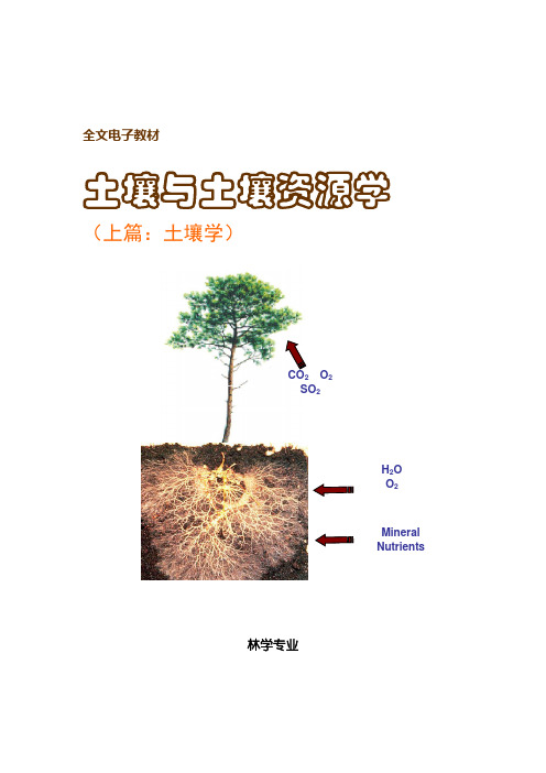
全文电子教材土壤与土壤资源学（上篇：土壤学）林学专业2 O 2SO2H 2OO 2MineralNutrients英文版—土壤养分Chapter 9. Soil NutrientsSoil nutrient availability is one of the factors that often limit tree growth and soil productivity. Other factors commonly limiting for tree growth can include soil moisture availability, climate (such as temperature and precipitation), soil physical properties (such as drainage and soil compaction), or a combination of the above factors. N is often a nutrient that is most deficient for plant growth. Nitrogen deficiency can be caused by low N content in the soil or by the slow release rate in ecosystems such as the boreal forests or peatlands where low temperature or poor aeration encourages accumulation of organic matter and reduces N mineralization rates. Phosphorus is also frequently deficient in soils where there is very little P in the parent material or where most of the P has been lost through weathering during the soil formation processes, such as in the tropics.There are 16 elements that are considered essential for plant growth. Lack of any of those essential nutrients will hinder the proper growth and functioning of the plants and will prevent the plants from completing their life cycle. Among those 16 essential nutrients, C, H, and O come from the air and water and are usually not deficient, although recent climate change studies using CO2 enriched air showed that increasing atmosphere CO2 concentration can significantly increase forest productivity; however, plants usually acquire the other essential nutrients from the soil. Among the macronutrients (N, P, K, Ca, Mg, and S), Mg and S can also sometimes be deficient for tree growth. Potassium and calcium deficiencies in forests are very rare. In terms of micronutrients (Mn, Zn, Cu, Fe, Mo, B, and Cl), B, Zn, Cu, and Fe deficiencies, especially B deficiency, are most frequently reported. These nutrients are called micronutrients because they usually exist on the earth and are required by plants in very small quantities. In addition to those 16 essential nutrients, cobalt (Co), vanadium (Va), nickel (Ni), silicon (Si), and sodium (Na) have been found to be essential to some plants. For example, nickel has been found to be essential for soybeans and Si for rice. In this chapter, we will discuss the importance of soil nutrients in tree growth, discuss the macronutrients and micronutrients, describe the cycling of nutrients in the soil, and provide an introduction to the mechanisms of plant nutrient uptake.9.1 Nutrients: available forms, availability and functionalityThe interaction of numerous physical, chemical, and biological properties in soils controls the availability of soil nutrients for plant uptake. Understanding these processes will enable us to manage selected soil properties to optimize nutrient availability and soil productivity. To understand these interacting processes will require us to have a good knowledge of the soil properties and processes covered in the earlier chapters. Not all nutrients present in the soil are available for plant uptake and different nutrients have different available forms.a) Forms of nutrients plant can uptakeDetails of available nutrient forms will be discussed in the next section where the individual macro- and micronutrients are presented. The forms of the essential nutrients that plants can uptake, along with their functionality and normal amounts in plants, are listed in Table 11.1. One thing common to all nutrients is that plants acquire most of their needed nutrients from the soil solution and mostly in the inorganic form. Some acquisition of nutrients through the gaseous form is possible. For example, plants can absorb NH3 and SO2 in the air through the stomata. Nitrogen cycling is one of the most complex as compared with the cycling of the other essential nutrients. One of the important mechanisms for increasing plant N availability is through symbiotic N-fixation. With this mechanism, most of the N the host plant uptake comes from the bacterial that can fix N2 in the air. There have been reports to indicate that trees sometimes can take up organic N in the form of simple amino acids and proteins. The uptake of organic form of N has been found to be mostly assisted by mycorrhizas and this uptake mechanism is very important in soils with low fertility and for nutrients with low mobility in the soil. A few species of plants are able to use animal proteins as an N source directly. These carnivorous plants, such as the common bladderwort (Utricularia vulgaris) and the sundew (Drosera rotundifolia), have special adaptations that are used to lure and trap insects and other very small animals. The plants digest the trapped organisms, absorbing the nitrogenous compounds the organisms contain as well as other compounds and minerals, such as potassium and phosphate. Most of the carnivores of the plant world are found in bogs, a habitat that is usually quite acidic and thus not favorable for the growth of nitrifying bacteria.b) Nutrient availabilityNutrient availability is an important area of interest in soil nutrient management. Nutrient availability falls into the soil science discipline of soil fertility. Soil fertility is narrowly defined as “the status of a soil with respect to the amount and availability to plants of elements necess ary for plant growth”. Of all soil properties, fertility is the one with which man is most involved; it is the property that can be readily changed by man in his exploitation or management of the land. In intensively managed forest systems, such as in plantations, soil nutrient availability can be altered and managed through silvicultural techniques such as site preparation, weed control, thinning, and fertilization. Even in natural forests, where there is very little human control of processes, soil nutrient availability is not a completely stable factor but changes with stage of forest succession, natural disturbance regimes, and with soil profile development. Occurrence of fire and extensive wind throw can result in sudden dramatic changes in soil nutrient availability. A soil, particularly one with the heterogeneity of many forest soils, cannot be considered to have a unique single, static level of soil fertility.Since plants take up most of their needed nutrients from the soil solution, nutrient availability is controlled by the interaction of numerous physical, chemical, and biological properties in soils. The basic relationship between the various components of the dynamic soil system is depicted in Figure 11.1. In reactions 1 and 2, plants absorb nutrients (cations and anions) from the soil solution and release small quantities of ions such as H+ (to balance the charge in soil solution, ifcations are absorbed by plants), or OH- and HCO3- (if anions are absorbed). In reactions 3 and 4, changes in ion c oncentrations in soil solution are “buffered” by ions adsorbed on the surface of soil minerals. Ion removal from solution causes partial desorption of the same ions from these surfaces. In reactions 5 and 6, minerals contained in the soil can dissolve to re-supply soil solution with many ions; likewise, increases in ion concentration in soil solution resulting from fertilization or other inputs can cause some minerals to precipitate. In reactions 7 and 8, soil microorganisms can remove ions from soil solution and incorporate them into microbial tissues, and conversely, when microbes or other organisms die, they release nutrients to the soil solution. Microbial activity produces and decomposes organic matter or humus in soils. These dynamic processes are very dependent on adequate energy supply from organic C, inorganic ion availability, and numerous environmental conditions. In reactions 9 and 10, plant roots and soil organisms utilize O2 and respire CO2 through metabolic activities. As a result, CO2 concentration in the soil air is greater than in the atmosphere. Diffusion of gases in soil decreases dramatically with increasing soil water content and soil depth. In reactions 11 and 12, numerous environmental factors and human activities can influence ion concentration in soil solution, which reacts with the mineral and biological processes in soil. For example, adding ammonium fertilizer to soil can increase the N concentration in the soil solution, but over time, N concentration in the soil solution will decrease due to plant uptake, volatilization losses, transformation of ammonium into nitrate through the nitrification process, and immobilization of ammonium by microorganisms and fixation by clays and organic matter through inorganic reactions.All of these processes and reactions are important to the availability of plant nutrients; however, depending on the specific nutrient, some processes are more important than others. For example, microbial processes are more important to N and S availability than mineral surface exchange reactions, whereas the opposite is true for K, Ca, and Mg.c) Functions of inorganic nutrients in plantsTable 9.1 lists some of the functions of nutrients in plant growth and physiology. Inorganic ions affect osmosis and thus help to regulate water balance in plants. Several inorganic ions can serve interchangeably in this role, in many plants this particular requirement is described as non-specific. On the other hand, an inorganic nutrient may function as part of an essential biological molecule; in this case the requirement is highly specific. An example of a specific function is the presence of magnesium in the chlorophyll molecule. Some of the common functions of mineral nutrients are discussed below.Catalysts: A key role of the inorganic nutrients is their participation in some of the enzymatic reactions of the plant cell. In some cases, they are essential structural parts (a “prosthetic group”) of the enzyme. In other cases, they serve as activators or regulators of certain enzymes. Potassium, for instance, which probably affects 50-60 enzymes, is believed to regulate the conformation of some proteins. Changing the shape of an enzyme could, for example, expose or obstruct reaction sites.Electron transport:Many of the biochemical activities of cells, including photosynthesis and respiration, are oxidation-reduction reactions. In such reactions, electrons are transferred to or from a molecule that functions as an electron acceptor or donor. The cytochromes, which contain iron, are involved in electron transfer.Structural and molecular components:Some mineral elements serve as structural components of cells, either as part of a physical structure or as part of the molecules involved in cellular metabolism. Calcium combines with pectic acid in the middle lamella of the plant cell wall. Phosphorus occurs in the sugar-phosphate backbone of DNA and RNA and in the phospholipids of the cellular membranes. Nitrogen is an essential component of amino acids, chlorophylls, and nucleotides. Sulphur is found in two amino acids that form a component of proteins.Osmosis:The movement of water into and out of plant cells is largely dependent on the concentration of solute in the cells and in the surrounding medium. The uptake of ions by a plant cell thus may result in the entry of water into the cell. The increased turgor pressure results in expansion of the immature cell, which is the chief cause of cellular growth, and in the maintenance of turgor in the mature cell. This is an example of conversion of energy from one form to another by a living system; the chemical energy (ATP) expended in the active uptake of ions by the plant cell is translated into the physical energy of water movement.Effects of cell permeability: Calcium has a direct effect on the physical properties of cellular membranes. When there is a calcium deficiency, membranes seem to lose their integrity, and solutes within the membranes or cells leak out.9.2 Macronutriens: N, P, K, Ca, Mg, and S9.2.1 Nitrogena) Origin and distribution of NThe N in soil is derived from the earth’s atmosphere. The N content of surface mineral soils typically ranges from 0.02 to 0.5%. About 98% of the earth’s N is contained in the igneous rocks deep under the planet’s crust, where it i s effectively out of contact with the soil-plant-air-water environment in which we live. Therefore, we must concentrate our discussion of N cycling on the remaining 2% that cycles in the biosphere. Most of the N found in the soil comes from biological N fixation. The atmosphere contains a large amount of N2 (78% of the atmosphere is N2 gas). Some 75,000 Mg of N is found in the air above 1 ha of the land surface. However, the very strong triple bond between two nitrogen atoms makes this gas quite inert and not directly usable by plants or animals. Were it not for the ability of certain microorganisms to break this triple bond to form nitrogen compounds, vegetation in the terrestrial ecosystems around the world would be rather sparse, and little N would be found in soils.Most of the N in terrestrial ecosystems is found in the soil. The soil contains 10 to 20 times as much N as does the standing vegetation (including roots) of forest ecosystems. Most soil N occurs as part of organic molecules. Soil organic matter typically contains about 5% N; therefore, the distribution of soil N closely parallels that of soil organic matter. Except where large amounts of chemical fertilizers have been applied, inorganic N (NH4+ and NO3-) seldom accounts for more than 1 to 2% of the total N in the soil. Unlike most of the organic N, the mineral forms of N are mostly quite soluble in water and may be easily lost from soils through leaching and volatilization.b) Forms of N in the soilThe different forms of N that can be found in the soil can be divided into two categories: inorganic and organic forms of N. As discussed above, most of the soil N exists in the organic form.Inorganic N: Inorganic forms of N include ammonium (NH4+), nitrate (NO3-), nitrite (NO2-), nitrous oxide (N2O), nitric oxide (NO), and the nitrogen gas (N2). Trace amounts of nitrite may be present in the soil. Nitrite is toxic to plants and is generally quickly converted to nitrate in the nitrification processes. Therefore, nitrite usually does not accumulate in the soil. N2O, NO, and N2 are the products of dinitrification or contained in the air trapped in the soil pores. As will be discussed below, conditions in forest soils generally favor the formation of ammonium and plants are adapted to this dominant form of N as a N source. Ammonium is the product of mineralization of organic N. Nitrate is formed through the nitrification process. There is usually abundant nitrate accumulation in the soil where conditions favor nitritication. The inorganic N content in soils is very dynamics as its concentration is affected by a large number of factors, including temperature, moisture content, plant uptake, microbial population, organic matter content, and so on. There are distinct seasonal and diurnal changes in soil inorganic N contents in the soil.Both inorganic N forms are soluble in water. Ammonium is mainly present in the soil on exchangeable sites and the positively charged ammonium can be attracted on to the negatively charged surfaces of clay and organic particles. This mechanism presents NH4+ from being easily lost from the soil solution. NH4+ can also be fixed in the clay structure, making it unavailable for plant uptake as well as from being lost through leaching. On the other hand, most of the NO3-, if present, will be found in the soil solution and is much more proven to be lost through leaching.Organic N: Organic N usually represent greater than 95% of the total soil N. Organic N occurs as proteins, amino acids, and other complex N compounds. Organic N can be separated into three types based on their solubility and how easy they can be hydrolyzed: a) soluble organic N: usually less than 5% of the total soil N content. Some of the soluble organic N (such as simple amino acids) can be take up directly by plants, especially with the assistance of mycorrhizas. This fraction of the organic N can be easily hydrolyzed to release NH4+ for plant uptake; b) hydrolyzable organic N. This fraction of organic N can be hydrolyzed to simpler soluble organic N when treated with acids or alkalis; and c) non-hydrolyzeable organic N. The content of this fraction can be as high as 50% of the total N in the soil. This is the most stable fraction of the soil organic N and the nature of this fraction of N is still not very clear. Much of the organic N forms organo-mineral complexes. Organic N in these complexes are much more stable than the non-complexed organic N in the soil.c) N cycling processesThe processes of N cycling are presented in Figure 11.2. The main N cycling processes are discussed below.Biological N fixation:Through biological N-fixation, certain organisms convert the inert dinitrogen gas of the atmosphere to N-containing organic compounds that become available to all form of life through the N cycle. Terrestrial ecosystems have been estimated to fix 130 to 180million Mg of N, about twice as much as is industrially fixed in the manufacturing of fertilizers.Symbiotic bacteria (Rhizobia) fix N2 in nodules present on the roots of legumes. This fixed N may be utilized by the host plant, excreted from the nodule into the soil and be used by other nearby plants, or released as nodules or legume residues decompose after the plant dies or is incorporated into the soil. Other microorganisms that are also capable of fixing N include Actinomycetes and Frankia that fix N in symbiosis with non-legume tree species such as alders, Myrica, and Casuarina; Azotobacter and Azospirillum are heterotrophic free-living fixers; and blue-green algae and Anabaena are autotrophic free-living fixers.Regardless of the organisms involved, the key to biological N fixation is the enzyme Nitrogenase, which catalyzes the following reaction:(Nitrogenase)N2 + 8H+ + 6e- ® —————————→2NH3 + H2(Fe, Mo)The nitrogenase are proteins that contain Fe and Mo. The nitrogen fixation process requires a great deal of energy. The energy either comes from the host plant for organisms that form symbiosis, or from the soil organic matter for the heterotrophic free-living bacteria, or from the sun light for the autotrophic free-living organisms. The accumulation of ammonia will inhibit N fixation and too much nitrate in the soil will inhibit the formation of nodules. In addition to Fe and Mo, N-fixing organisms also require high amounts of P and S as these nutrients are either part of the nitrogenase molecule or are needed for its synthesis and use.The production of N by industrial fixation is based on the Haber-Bosch process, in which H2 and N2 gases react to form NH3, under high temperature and pressure:Catalyst3H2 + N2 ® ——————→NH31,200 °C, 500 atmImmobilization and mineralization: The majority (95-99%) of the soil N is in organic compounds that protect it from being lost but this also leaves it largely unavailable to higher plants. The quantities of NH4+ and NO3- available to plants depend largely on the amounts applied as N fertilizers and mineralized from organic N in soil. Much of the organic N is present as amine groups (R-NH2), largely in proteins or as part of humic compounds. When soil microbes attack these compounds, simple amino compounds (R-NH2), such as lysine (CH2NH2COOH) and alanine (CH3CHNH2COOH), are formed. Then the amine groups are hydrolyzed, and the N is released as ammonium ions (NH4+), which can be oxidized to the nitrate form. This enzymatic process is termed mineralization, that includes the ammonification (from simple amino compounds to NH4+) and nitrification (from NH4+ to NO3-) processes. A specific term called aminization describes the process from the amine groups and proteins to simple amino compounds:H2OProteins ® RCHNH2COOH + R-NH2 + CO(NH2)2 + CO2 + energyBacteria, fungiUsing an amino compound (R-NH2) as an example of the organic N source, the mineralization process can be indicated as follows:+2H2O +O2 +1/2O2R-NH2 ⇌OH- + R-OH + NH4+ ⇌4H+ + energy + NO2- ⇌energy + NO3--2H2O -O2 -1/2O2The opposite of the mineralization process is immobilization, the conversion of inorganic N ions (NH4+ and NO3-) into organic forms. Immobilization can take place by both biological and non-biological (abiotic) processes, the latter being of considerable importance in forest soils. Through the biological processes, as microorganisms decompose carbonaceous organic residues in the soil, they may require more N than is contained in the residues themselves and thus may immobilize NH4+ and NO3- in the soil solution. The microbes need N to maintain a C:N ratio of about 8:1. The microorganisms incorporate mineral N ions into their cellular components, such as proteins, leaving the solution essentially void of NO3- and NH4+ ions. During the immobilization process, microorganisms can compete very effectively with plants for NH4+ or NO3-. When the organisms die, some of the organic N in their cells may be converted into forms that make up the humus complex, and some may be released as NH4+ and NO3- ions. During the decomposition of nitrogenous compounds, microorganisms incorporate the N into amino acids and proteins (as part of the microbial biomass) and release excess N in the form of ammonium ions. In alkaline media, the N may be converted to ammonia (NH3), but this conversion usually occurs only during the decomposition of large amounts of N-rich material, as in the mature pile or a compost heap that has contact with the atmosphere. Within soil, the ammonia produced by ammonification is dissolved in the soil water, where it combines with protons to form the ammonium ions. Mineralization and immobilization occur simultaneously in the soil; whether the net effect is an increase or decrease in the amount of mineral N available in the soil depends primarily on the ratio of C to N in the organic residues undergoing decomposition.The amount of plant available N released from organic N depends on many factors affecting N mineralization, immobilization, and losses of NH4+ and NO3- from the soil. Mineralization being a microbial process will increase with a rise in temperature and is enhanced by adequate, although not excessive, soil moisture and a good supply of O2. Maximum aerobic activity and N mineralization occur between 50 and 80% water-filled pore space. Optimum temperature for N mineralization ranges between 25 and 35 °C.One of the factors affecting N mineralization and immobilization is the C:N ratio of the decomposing material. The N content of humus or stable soil organic matter ranges from 5 to 6%, whereas C ranges from 50 to 60%, giving a C:N ratio ranging between 8 and 12. When fresh organic material is added to the soil, there is a rapid increase in the number of heterotrophic organisms, accompanied by the evolution of large amounts of CO2, during the initial stage of decomposition. If the C:N ratio of the initial material is greater than 30:1, N immobilization occurs. As decay proceeds, the C:N ratio of the residue narrows and energy supply diminishes.Some of the microbial population dies because of the decreased food supply, and ultimately a new equilibrium is reached, accompanied by the mineralization of N. Generally speaking, when organic substances with C:N ratios between 20 and 30 are added to the soil, there may be neither immobilization nor release of mineral N. For organic materials with C:N ratio less than 20, there is usually a release of mineral N early in the decomposition process.In the organic matter mineralization processes, bacteria dominate the breakdown of proteins in neutral and alkaline environments, with some involvement of fungi, while fungi predominate under acidic environments (and most forest soils are acidic).Many studies have shown that only about 1 to 4% of the organic N of a soil mineralizes annually. Even so, the rate of mineralization provides sufficient mineral N for normal growth of natural vegetation (such as forests) in almost all soils except those with low organic matter, such as the soils of deserts and sandy areas. Mineralized soil N constitutes a major part of the N taken up by plants.Nitrification: Several species of bacteria common in soils are able to oxidize ammonia or ammonium ions in a process called nitrification. This is an energy yielding process, and the energy released in the process is used by these bacteria to reduce CO2 in much the same way that photosynthetic autotrophs use light energy in the reduction of CO2. Such organisms are known as chemosynthetic autotrophs (as distinct from photosynthetic autotrophs). The chemosynthetic nitrifying bacterium Nitrosomonas is primarily responsible for oxidation of ammonium to nitrite ions (NO2-).Nitrosomonas2NH4+ + 3O2 ® 2NO2- + 4H+ + 2H2O + energybacteriaNitrite is toxic to plants, but it rarely accumulates in the soil. Nitrobacter, another genus of bacteria, oxidizes the nitrite to form nitrate ions (NO3-), again, with a release of energy:Nitrobacter2NO- + O2 ® 2NO3- + energybacteriaOnce nitrate is formed and if it is not quickly taken up by plants or microbial organisms (in the process of microbial immobilization), it can be lost from the soil through leaching, when there is water percolating through the soil profile, and denitrification under anaerobic conditions. Nitrification will significantly increase soil acidity by producing H+ ions. Nitrification requires NH4+ ions, but excess NH4+ is toxic to Nitrobacter and must be avoided. The nitrifying organisms, being aerobic, require O2 to make NO2- and NO3- ions, and are therefore favored in well-drained soils.In forest soils, fortunately, nitrification rates are very low and most of the available form of N is present in the ammonium ion form. There are several possibilities that nitrification rates are low in forest soils. One possibility is that nitrification rates are inhibited by the low soil pH as forest soils are usually acidic. A second possibility is that nitrifying bacteria population is very low (that itself may be related to the inhibition by the acidic condition and other limiting factors) in forestsoils. Under prolonged incubations in the lab, nitrification eventually develops, although this may take as long as one year under optimum conditions. Another possibility is that microbial populations in forest soils have a very strong ability to immobilize the nitrate produced from nitrification. Therefore, under such a scenario, as soon as the nitrate is formed the microbial populations take it up. Recent gross N mineralization studies using 15N-labeled fertilizers confirmed such cases.Nitrification is also a microbial process and is thus affected by soil environmental factors. Nitrification is affected by 1) soil NH4+ content, 2) population of nitrifying organisms, 3) soil pH, 4) soil aeration, 5) soil moisture, and 6) temperature. If there is no NH4+ in the soil solution, nitrification does not occur. Variation in populations of nitrifiers results in differences in the lag time between the addition of the NH4+ and the buildup of NO3-. Because of the tendency of microbial populations to multiply rapidly in the presence of an adequate supply of C, the total amount of nitrification is not affected by the number of organisms initially present, provided that temperature and moisture conditions are favorable for sustained nitrification.Nitrification takes place over a wide range in pH (4.5 to 10), with an optimum pH of 8.5. Nitrifying bacterial need an adequate supply of Ca2+, H2PO4-, and a proper balance of micronutrients. Nitrifying bacteria are aerobes and maximum nitrification occurs at the same O2 concentration in the aboveground atmosphere. Nitrification rates are generally highest in soil water contents at field capacity or 1/3 bar water potential (80% of total pore space filled with water). In terms of temperature, the temperature coefficient, Q10, is 2 over the range 5 to 35 °C. Thus, a twofold change in the nitrification rate is associated with a shift of 10 °C within this temperature range. Optimum soil temperature for nitrification is 25 to 35 °C.Nitrate leaching:Nitrate ions are not adsorbed by the negatively charged colloids that dominate most soils. Therefore, nitrate ions move down easily with drainage water and are thus readily leached from the soil. This process constitutes a loss of N from the soil system for plant uptake and also causes several serious environmental problems. Leaching of nitrate from acidic sources (nitrification or acid rain) also facilitates the loss of Ca and Mg and other nutrient cations. Much of the nitrate mineralized in certain highly weathered, acid, tropical Oxisols and Ultisols leach below the root zone before annuals can take it up. It has been found that some of this leached nitrate is not lost to groundwater, but is stored several meters deep in the profile where the highly weathered clay have adsorbed it on their anion exchange sites. Deep-rooted trees are capable of taking up this deep subsoil nitrate and subsequently using it to enrich the surface soil when they shed their leaves. Trees such as Sesbania, grown in rotation with annual food crops, can make this pool of leached N available for food production and prevent its further movement to ground water. Agroforestry practices such as this have the potential to make a significant contribution to both crop production and environmental quality in the humid tropics.Ammonium fixation: Ammonium ions carry positive charges and thus can be attracted to the negatively charged surfaces of clay and humus, where they are held in exchangeable form, available for plant uptake, but partially protected from leaching. However, because of the particular size of the ammonium (and potassium) ion, it can become entrapped within cavities in the crystal structure of certain clays. Several 2:1 type clay minerals, especially vermiculites, have the capacity to fix both ammonium and potassium ions in this manner. Vermiculite has the greatest capacity, followed by fine-grained micas and some smectites, to fix ammonium and potassium in this manner. Ammonium and potassium ions fixed in the rigid part of a crystal structure are held in。

Plant and Soil(2005)268:21–33©Springer2005 DOI10.1007/s11104-005-0175-5The effect of soil water content,soil temperature,soil pH-value and the root mass on soil CO2efflux–A modified modelSascha Reth1,3,Markus Reichstein2&Eva Falge11Department of Plant Ecology,University of Bayreuth,D-95440Bayreuth,Germany.2Potsdam Institute for Climate Impact Research Natural Systems Department,D-14473Potsdam,Germany.3Corresponding author∗Received10February2004.Accepted in revised form21April2004Key words:fine-root mass,non-linear regression model,pH respiration,soil moisture,soil temperatureAbstractTo quantify the effects of soil temperature(T soil),and relative soil water content(RSWC)on soil respiration we measured CO2soil efflux with a closed dynamic chamber in situ in thefield and from soil cores in a controlled climate chamber experiment.Additionally we analysed the effect of soil acidity andfine root mass in thefield.The analysis was performed on three meadow,two bare fallow and one forest sites.The influence of soil temperature on CO2emissions was highly significant with all land-use types,except for onefield campaign with continuous rain. Where soil temperature had a significant influence,the percentage of variance explained by soil temperature varied from site to site from13–46%in thefield and35–66%in the climate chamber.Changes of soil moisture influenced only the CO2efflux on meadow soils infield and climate chamber(14–34%explained variance),whereas on the bare soil and the forest soil there was no visible effect.The spatial variation of soil CO2emission in thefield correlated significantly with the soil pH andfine root mass,explaining up to24%and31%of the variability.A non-linear regression model was developed to describe soil CO2efflux as a function of soil temperature,soil moisture,pH-value and root mass.With the model we could explain60%of the variability in soil CO2emission of all individualfield chamber measurements.Through the model analysis we highlight the temporal influence of rain events.The model overestimated the observedfluxes during and within four hours of the last rain event. Conversely,after more than72h without rain the model underestimated thefluxes.Between four and72h after rainfall,the regression model of soil CO2emission explained up to91%of the variance.IntroductionSoil CO2fluxes are the second major component of the global carbon cycle(Reich and Schlesinger1992), and play an important role in climate change.Very often is it hypothesized that soils provide a positive feedback to climate warming due to the exponential response of soil CO2efflux to temperature(e.g.Cox et al.,2000;Kirschbaum,1995).However,the gas ex-change between the soil and the atmosphere depends on numerous complex and non-linear relationships, like physiological,biochemical,chemical,ecological and meteorological conditions(Jarvis,1995;Schimel et al.,1994).Soil respiration represents the biolog-ical activity of the entire soil biota,including soil ∗FAX No:+490921552061microbes(e.g.bacteria,fungi,algae,protozoa),plant roots and macroorganisms(e.g.earthworms,nema-todes,insects).The rates of soil CO2efflux vary by ecosystem(Reich and Schlesinger,1992)and are the major component of whole-ecosystem respiration,that in turn explains much of the continental gradient of the net carbon balance(Schulze et al.,1999;Valen-tini et al.,2000).So show Kelliher et al.(1999)and Law et al.(1999b)for forested ecosystems,that soil respiration amounts to76–77%of the annual GPP, whereas agricultural crops during fallow periods act as a carbon emitter(Soegaard,1999;Soegaard,et al. 2003).Despite these general trends emissions of CO2 are highly spatially variable within one site(Law et al., 2001;Longdoz et al.,2000;Simek et al.,2004).22A positive correlation between soil temperature and soil CO2efflux is well described by several re-views(Kätterer et al.,1998;Lloyd and Taylor,1994; Reich and Schlesinger,1992;Singh and Gupta,1977). Also,soil moisture affects the soil CO2efflux(Bun-nell et al.,1977;Orchard and Cook,1983;Reichstein et al.,2002;Simek et al.,2004;Subke et al.,2003). Furthermore,soil CO2efflux is influenced by other factors like,substrate amount(Zak et al.,2000),the pH-value of the soil(Hall et al.,1997)as well as the activity of the vegetation(Reichstein et al.,2003b) since root respiration(Janssens et al.,1998;Kutsch et al.,2001;Law et al.,1999a)and heterotrophic res-piration(Goulden et al.,1996;Hollinger et al.,1998) comprise total soil CO2efflux,and plants continu-ously excrete exudates into the soil.Several studies showed significant effects of soil pH values on soil respiration(Andersson and Nilsson,2001;Hall et al., 1997;Sitaula et al.,1995)since,in particular,mi-crobial activity increases with rising pH values(Ellis et al.,1998).Furtheron,temporal effects like litter fall,decom-position dynamics and the amount and the timing of rainfall(Ball et al.,1999;Jackson et al.,1998)influ-ence soil respiration.The effect of rainfall was often larger than expected from the relationship between soil moisture and CO2efflux(Davidson et al.,1998; Russell and V oroney,1998).A series of models try to explain the relation-ship between the factors governing soil CO2ef-flux.Most studies use different principles to describe temperature effects, e.g.linear regression analysis (Witkamp,1966),Q10(Maljanen et al.,2002;Reich and Schlesinger,1992)or power relationship(Kucera and Kirkham,1971),as well as relationships based on the Arrhenius form(Howard and Howard,1979). However,all existing models cannot explain the total variation of the CO2soil efflux.Numerous empirical models were developed for crop(Boegh et al.,1999) and meadow soils(Bremer and Ham,2002)or bare soils(Gupta et al.,1981;Reth et al.,2004).These models are not useful for forest soils.In contrast forest models(Baldocchi and Wilson,2001;Janssens et al., 2001;Nakano et al.,2004;Rasse et al.,2001)are often of low use at bare soil or meadows.The aim of this study is to analyse the influence of soil temperature,moisture,pH value and root mass on soil CO2efflux through a combination offield and lab-oratory experiments.In a second step these effects are assembled into an empirical model that should work on meadow and cropland as well as in forest and bare fallow soil.Finally,we explore a robust regression method to identify temporal effects on soil CO2efflux in thefield that are not represented by the model. MethodsSite descriptionThe measurements used in this study were carried out in the course of special observation periods of the VERTIKO(Vertical transport under complex natural conditions)project,which is part of the AFO2000 (German Atmospheric Research,2000)programme. The target area of the VERTIKO project comprises the region between the Erzgebirge in the South and the Oder-Spree lake district in the North(100km WE and 300km NS).It includes a variety of natural small-scale variability from land use to orographic effects typical for Germany.During three special observation periods (SOPs)measurements were performed at anchor sta-tions located in the target area.For an overview of the parameters observed during thefield campaigns that are expected to influence soil CO2efflux see Table1.The measurements of SOP1were carried out in September and October2001at the Anchor Station Melpitz of the Institute for Tropospheric Research,lo-cated near Melpitz,Saxony(51◦31 N,12◦55 E,86m a.s.l.).The area is aflat managed meadow(MW)of approximately20ha surrounded by farmland(MA, see e.g.Spindler et al.,2001).The annual mean air temperature is8.7◦C and the annual precipitation 539mm.The dominant species were Lolium perenne, Taraxacum officinale and Leontodon autumnalis.The leaf area index(LAI)was2.0m2m−2.The SOP2experiment took place in June and July2002at the Falkenberg Boundary-Layer mea-surement site of the German Meteorological Service, the Lindenberg observatory,Brandenburg(52◦10 N, 14◦07 E,73m a.s.l.).The landscape in this region was formed by inland glaciers of the last ice age, with a slightly undulating orography and a hetero-geneous land use structure(see e.g.Beyrich et al., 2002).The Falkenberg site itself isflat and consists of about18ha of managed meadow(LW)with short grass.An area of approximately3ha of the meadow was ploughed during the experiment(LA).The annual mean air temperature is8.6◦C and the annual precip-itation560mm.Main species were Lolium perenne, Bromus hordeaceus,Festuca rubra,Leontodon autum-nalis,Taraxacum officinale,Trifolium pratense and23 Table1.Observed range of the parameters T soil(soil temperature),RSWC(relative soil watercontent),pH and RRM(fine root biomass,d.w.based)expected to influence soil CO2emissionduring thefield campaigns(MW=Melpitz Meadow,MA=Melpitz Agricultural Fallow,LW=Lindenberg Meadow,LA=Lindenberg Agricultural Fallow,TW=Tharandt Meadow,TF=Tharandt Forest)T soil T soil RSWC RSWC pH pH RRm RRMmin(◦C)max(◦C)min(%)max(%)min max min(%)max(%)MW10.316.6398 5.87.10.0359MA10.721.53999 6.97.400LW14.325.81738 4.5 6.90.4126LA14.518.91617 5.0 5.900TW11.520.95897 5.0 5.526TF9.018.65681 3.3 3.80.3636Trifolium repens.Meadow LAI showed a spatial gra-dient during thefield campaign,with maximum LAI of4.7,and minimum LAI of1.3m2m−2.The SOP3measurements were performed in May and June2003at the Anchor Station Tharandter Wald of the Technical University Dresden near Tharandt, Saxony(50◦58 N,13◦34 E,375m a.s.l.).The slightly undulating experimental area is located inside a closed forest of approximately6000ha.The annual mean air temperature is7.6◦C and the annual precipita-tion820mm.The forest(TF)is dominated by114 years old,approximately28m high Picea abies(L.) KARST trees.The projected leaf area index(LAI) was6.9m2m−2.The meadow area(TW)of the anchor station is1.5ha and dominated by Rumex ob-tusifolium(L.),Holcus lanatus(L.),Cirsium arvense (L.)and Carex spp.The leaf area of the meadow was 2.6m2m−2at the beginning(May,22)of theflux measurements and increased to6.1m2m−2at the end of the campaign(June,13).Thesefield measurements were complemented by climate chamber experiments to extend the range of soil temperatures and soil moisture observed during the SOPs.Soil efflux and soil analysis in thefieldSoil CO2efflux was measured with a non-steady-state flow-through chamber system,andfluxes were deter-mined from the concentration increase in closed cham-bers.The system consists of cylindrical steel chambers (height80mm and diameter197mm)with plexi glass lids attached during the measurement.No fan was used in the system.Overheating could be avoided because single measurements were completed within12min,and soil temperatures inside and outside the chamber differed less than0.2◦C.The chambers were inserted 2cm into the soil and all plant material was removed from the chambers’interiors.Thefirstflux measure-ments started approximately12h after plant cutting to avoid effects on soil CO2efflux by collar inser-tion or plant cutting.Collars remained in place during all subsequent measurements at the site.Ten cham-bers were installed as spatial replicates at each land use type,except at the bare soil of Lindenberg with onlyfive chambers.Measurements took place from the early morning to late in the evening.The chambers were moved to another site or land use afterfinishing 5to14measurements at the same point.The sys-tem allowed to measurefive chambers alternately with magnetic valves controlling theflow of the different chambers.For the concentration measurements the air was pumped in a closed loop from the chamber to the analyser(Photoacoustic Multi-gas Monitor,INNOV A 1312)and back to the chamber.Through a20m long tube with an inside diameter of3mm,the air was sucked for approximately30s with a speed of4m s−1. The concentrations of CO2(for control)and water were determined from the air stream.The CO2efflux was determined from the slope of the concentration increase within a chamber using four concentrations measured at238s intervals.The system was tested against other measurement systems(non-steady-state flow-through chambers,non-steady-state non-flow-through chambers,non-steady-state non-flow-through chambers and a calibration system)in a calibration experiment(Pumpanen et al.,2004).In this experi-ment he system employed showed an underestimation of approximately4%for soils comparable to those in this study,and at maximum11%for dryfine sand.24Parallel to the soilflux measurements environ-mental parameters were observed quasi-continuously. Soil temperature(Thermistor,Siemens M841)was recorded at2cm depth inside each chamber and out-side the chambers every5min.V olumetric soil water content(SWC,m3water per m3total soil volume, Theta Probe,ML2)was measured half hourly in the upper10cm of the soil at each stand.Relative soil wa-ter content(RSWC)is defined as SWC divided byfield capacity,allowing for a better comparison of soils with different textures.Reichstein et al.(2002)found very similar RSWC1/2parameters for a sandy and clayey soil,Nevertheless one would not expect exactly the same values of RSWC1/2in all soils,and our assump-tion that reduces the number of model parameters introduces(albeit little)model error.Analysis of root mass and pH of soil samples of each chamber were performed afterfinishingflux measurements.Soil cores with a diameter of5cm and a depth of10cm were taken in thefield,and soil and roots were separated manually.The remaining soil was sieved to remove stones.The root biomass was dried three days at105◦C.The dry mass of the roots was expressed per unit dry mass of the oven-dry soil.The pH-value was determined from a fresh soil slurry using a glass electrode(Scheffer and Schachtschabel,2002). Incubation time of20g soil was1h in50g distilled water.Soil efflux in the climate chamberFor the climate chamber experimentsfive replicate fresh soil cores(diameter=31cm,height=25cm) were collected under minimal disturbance from the meadow of Melpitz,Lindenberg and Tharandt as well as from the fallow of Lindenberg and the forest of Tharandt.CO2efflux of the soil samples was recorded over112days.Soil temperature was manipulated by changing the air temperature inside the climate chamber.Starting at20◦C the soil temperature was decreased every two days by2◦C.After reaching4◦C the soil temperature was increased every two days by 2◦C up to38◦C,then decreased again and so forth. Soil water content was altered by irrigation and drying cycles.At beginning and end of eachflux measure-ment(for description of the system see above),we weighed the soil cores for gravimetric determination of soil water content.In the climate chamber it was not possible to analyse the soil without destroying the soil cores.Therefore the soils were not analysed for the parameters pH and RRM.Soil CO2modelThe non-linear regression model of soil CO2efflux was adapted from Reichstein et al.(2003b,2002)that includes a function for soil temperature(T soil,Equa-tion3)–following an exponential response,a function of relative soil water content(RSWC,Equation4) and a function of vegetation activity.We modified the model by Reichstein(2003b)for better incorporation of the actually measured data in two ways:(1)The soil CO2emission rate under standard conditions,was made dependent on root mass per soil mass as a proxy for vegetation activity(instead of leaf area index in Reichstein,et al.2003b);(2)We included the influ-ence of soil chemistry through including the soil pH as additional predictor.Mathematically,the model is described by the following equations:R soil=R ref∗F(T soil)∗g(RSW C)∗h(pH),(1) where R soil is the soil CO2efflux.The emission under standard conditions(R ref),at T ref and non-limiting soil water content,is described by:R ref=H resp+a resp,(2) where h resp represents heterotrophic respiration and a resp autotrophic respiration.The heterotrophic respi-ration is afitted parameter and a resp is a linear function of the root mass per dry soil mass(RRM)and a parameter(rf):a resp=R RM∗r f.(3) The exponential increase of the CO2emission with soil temperature is described by:f(T soil)=expE0∗1T ref−T0−1T soil−T0,(4) where E0is a free parameter analogue to the activation energy in the standard Arrhenius model,T ref is the reference soil temperature and T0the lower temper-ature limit for R soil.T ref was set to15◦C and T0at −46.02◦C(Lloyd and Taylor,1994).The response of changes on relative soil water content is described by: g(RSW C)=RSW C−RSW C0(RSW C1/2−RSW C0)+(RSW C−RSW C0).(5)RSWC1/2represents the RSWC at half-maximum soil CO2efflux and RSWC0is the residual soil water con-tent,below which the efflux ceases.RSWC1/2and RSWC0are free parameters.Finally,the response of the CO2emission with soil pH-value follows an optimum curve:25 Table2.Coefficients of variation for the univariate analysis of soil CO2emission influencing parametersduring thefield(FM)and the climate chamber measurements(CCM).T soil(soil temperature),RSWC(relative soil water content),pH and RRM(fine root biomass,d.w.based),n represents the number ofCO2flux observations not affected by rain,and used for the regression model parameterisation.For siteabbreviations see Table1FM CCMT soil RSWC RRM pH n T soil RSWCMW0+0+0+0+00.45∗0.1MA0+0+ND0+00.35∗0.09LW0.25∗0.34∗0.12∗0.19∗1410.52∗0LA0.46∗0ND0.24∗30ND NDTW0.31∗0.18∗0.3∗0.19∗500.65∗0.14∗TF0.13∗0.040.31∗0.23∗740.66∗0P<0.01,ND=not determined.+not used for model parameterisation.h(pH)=exp−pH−phOptphSens2,(6)where phOpt is a free parameter and represents the optimal pH value.The parameter phSens describes the sensitivity of soil CO2efflux to deviation from this optimal value.Parameter estimationFor the data analysis with the non-linear regression model we used a robust regression technique that is able to objectively identify outliers,or more pre-cisely data points,that are inconsistent with the model assumptions.We used the non-linear least trimmed squares(LTS)regression(Reichstein et al.,2003a; Stromberg,1997),that seeks to minimize the sum of squared residuals as ordinary non-linear regression, but with exclusion of the largest x%of residuals,that are assumed to be due to contaminated data or due to data inconsistent with the model.Formally the objec-tive function that has to be minimised is the trimmed sum of squared errors(TSSE):T SSE=i≤N·(1−0.001−t)r2i,(7)where r i is the i-th smallest residual,N is the to-tal number of data points,and(0.01t)is the fraction of residuals to be excluded.The procedure was per-formed with trimming percentages of10,20,30% and subsequently analysed which data was classified as‘contaminated’by the procedure.ResultsWe examined the effect of soil temperature changes on CO2efflux at the four soil types of thefield mea-surements and offive soil types in the climate chamber experiment.Due to the continuous rain during SOP1, the results of thefield measurements in Melpitz were not used in the temperature,and all further analyses. An exponential increase with increasing soil tempera-ture was observed at all soils(Figure1),both during thefield measurements and in the climate chamber experiment(Table2).Meadow soils,except MW in bothfield and cli-mate chamber measurements,and LW in the climate chamber measurements,responded to changes of rel-ative soil water content.There was no statistically significant effect at the fallow and the forest soil,both in thefield and in the climate chamber measurements (Table2).Variation of the pH-value of the soils and between the single measurement points at each site showed a positive correlation with the CO2efflux(Figure2). During simultaneous measurements with similar soil temperature and soil water content,the chambers with higher soil pH exhibited higher CO2fluxes,except in Melpitz(Table2).Also the presence offine roots significantly af-fected the observed soil CO2efflux.At all meadow and forest stands,again except for Melpitz,the relative root mass was correlated positively(Figure3)with the CO2flux rates(Table2).While the univariate relationships between soil CO2efflux and environmental factors were gener-ally weak,the above soil CO2efflux model already26Figure1.Soil CO2efflux as an exponential function of soil temperature(T soil)for the meadow soil of Tharandt(TW)in thefield(closed dots, r2=0.31),and in the climate chamber(open dots,r2=0.65).The lines are regression lines,calculated from the used data using equation4.Figure2.Soil CO2efflux as function of soil pH-value at the fallow in Lindenberg(LA).Dots represent the mean CO2fluxes(n=5)with error bars(r2=0.24).The line is the regression line,calculated from the used data using equation6.27 Figure3.Soil CO2efflux as function of relative root mass(RMM)at the meadow soil of Tharandt(TW).Dots represent the mean CO2fluxes (n=6)with standard deviation(r2=0.30).The line is the regression line,calculated from the used data using equation3.explained60%of the variability of soil CO2efflux (Figure4a).With the robust regression approach we analysed inconsistence of the model(Figure4b–d). 30%of the data could be identified as inconsistent with the model and could be related to disturbance by precipitation events(Figure4e).Thereby we could identify3periods:During and up to4h after a rain event(period1)the model overestimated the measured CO2fluxes.In contrast, after a dry period of more than72h(period2)the model underestimated thefluxes.In the time period in between,that is4to72h after the last rain event (period3),the model reflected the measured emissions well,and explained91%of their variability(Table3). Interestingly,the amount of rain did not affect the per-formance of the model.The robust regression method rejected87%of the data points falling into period1or 3,supporting the rationale to identify and exclude data that are inconsistent with the model.DiscussionIn this paper we confirmed well known correlations of soil CO2efflux and abiotic factors,although some-times the ranges of driving forces in thefield were too small to detect previously reported effects,e.g.on Q10.The strong correlation of temperature and soil CO2 emission was quantified for many soils under different conditions(see e.g.Epron et al.,1999;Kätterer et al., 1998;Lloyd and Taylor,1994;Reich and Schlesinger, 1992).In our climate chamber measurements,all soils showed an exponential increase of soil CO2efflux with increasing soil temperature(P<0.01).In the field the soil CO2efflux was more variable,indicating increasing influence of other parameters.A similar distinction was observed comparing soil CO2exchanges at changing soil moisture.Only at the meadow stands in Tharandt and in thefield measure-ments of Lindenberg soil CO2efflux showed signifi-cant(P<0.01)response to soil moisture changes.At the other stands,and partly during the climate chamber experiments,the relative soil water content span al-lowed only for small limiting effects due to soil water. Also,Reichstein et al.(2003b)observed a broad range28parison of modeled and measured soil CO2efflux:(a)without a trimmed fraction(r2=0.60),(b)with a trimmed fraction of 10%(r2=0.80),(c)with a trimmed fraction of20%(r2=0.86),(d)with a trimmed fraction of30%(r2=0.91)and(e)evaluating the temporal effect of last rain event.Lines are1:1lines.29 Table3.Parameters of the nonlinear regression model for all stands with a trimmed fraction of30%(n=295).240values were not effected by rain or drought,and indicated as consistentwith the model(LW:n=97,LA:n=30,TW:n=44,TF:n=69).Root mean squareerror(RMSE)of the model results was0.89µmol m−2s−1.To take into account the4%underestimation of the system(Pumpanen et al.,2004),the parameters h resp and rf have to bemultiplied with the correction factor0.96Parameter Units Value Standard errorh respµmol m−2s−19.11 2.12E0K247.7816.84RSWC0%92RSWC1/2%170.9phOpt9.35 1.23phSens−4.870.69rfµmol m−2s−1g d.w.19.91 5.23Soil(g d.w.root)−1of near optimum soil water content where changes in soil moisture have little or no effect and correspond to our observations.At the bare soil of SOP2at Linden-berg the soil water content was nearly constant while the measurements were performed,so there was no effect of soil moisture changes on CO2efflux at this time.Even when taking soil temperature and water con-tent into account,the spatial variation of soil CO2 efflux at one site can be large.Buchmann(2000)re-ported spatial variations among soil collars,which were larger than the diurnal variability of soil CO2 emission rates measured with the same collars during a day.This corresponds well with ourfield measure-ments,in particular at the forest stand,where soil temperature changes were very small,but spatial vari-ability was high.Thus,multivariate interaction of various other factors has to be accounted for as in the model presented here.The link of respiration to vegetation productivity established by Reichstein et al.(2003b)with poten-tially confounding factors at the continental scale,was here confirmed at small scale for soil CO2efflux.An-derson(1992)and Janssens et al.(1998)showed,that root respiration may account for half of the soil efflux. In general,this agreed with our observations for the forest and meadow sites.In addition,samples with higher root mass per soil showed higher CO2emission (P<0.01)at comparable meteorological conditions. Thisfinding held within a site,but not among differ-ent sites,where other factors determined the overall magnitude of soil CO2efflux.An influence of spatial heterogeneity of soil pH on soil CO2emission was confirmed at all stands (P<0.01),except Melpitz.Several studies described a similar positive correlation of pH-value and soil CO2 efflux(Andersson and Nilsson,2001;Ellis et al.,1998; Hall et al.,1997;Sitaula et al.,1995).Baath(1996) and Högberg et al.(2003)demonstrated the direct pos-itive effect on soil respiration with pH tolerance of the bacterial community.A biological activity of soil microorganisms is permitted between a soil pH of a minimum of3and a maximum of7to8(Scheffer and Schachtschabel,2002).Between these values(see Ta-ble1),and otherwise constant conditions we observed a nearly linear increase of soil CO2emission.In the model however,we described the response to soil pH with an optimum curve to account for potential decline in soil CO2emission above a pH of9.Similar pattern were shown in Wittmann et al.(2004)with an opti-mum curve for the dependence of hydrolytic enzyme activities in a forest soil.The nonlinear regression model gave good results for all investigated sites.Up to60%of the data vari-ance could be explained by soil temperature,relative soil water content,soil pH and relative root mass. Evaluating the time span between measurement and last occurring rain,the modeled soil CO2effluxes overestimated the measuredfluxes in the case of rain or maximum4h after the last rain.The main cause for this could be the reduction of the soil air-filled pore space resulting in reduced gaseous diffusivities. The negative effect of waterfilled pores on soil CO2 emission is often discussed in the literature(see e.g. Ball et al.,1999;Lee et al.,2002).30After three or more days without rain,the model underestimated the observedfluxes.An explanation for this might be a shift of the main respiratory ac-tivity to deeper soil layers,with soil moisture and temperatures more favourable to respiration than those recorded by the sensors in the top soil layer.Another explanation could be thatfine roots dying in the upper soil,and new root development in deeper soil layers led to an increase in CO2release.For the time be-tween4and72h after a rain event,the model worked well,explaining91%of the soil efflux variation with changes in soil temperature,soil water content,root mass and soil pH.Potential limitation of the model could be that the temperature,soil water content,and pH responses of respiration arising from roots and soil heterotrophs might differ.Root respiration depends on current pho-tosynthetic products as substrate,and is therefore mainly controlled by light availability during the last2 days(Fitter et al.,1998).Heteorotrophs use older pho-tosynthetic products(e.g.litter,turnover offine roots), but also use root exudates(Grayston et al.,1997),as rhizosphere micro-organisms rapidly acquire the iso-topic signature of the current photosynthate(Pendall et al.,2003),therefore being partly coupled to light availability too.In our case,we had to simplify these effects,as it was not possible to separate the responses of these two componentfluxes from data measured with our technique.We included only the relative amounts of autotrophic and heterotrophic respiration in the model,and applied identical temperature,soil water content,and pH functions.We tried to overcome the limiting effects of rel-atively short measurement campaigns at the various sites with soil cores taken to the climate chamber for wider ranges of temperature and moisture.However, this setup still did not allow for proper assessment of threshold events or sudden shifts in key variables de-termining soil respiration or soil CO2efflux.Yet in the field,Jensen et al.(1996),Lee et al.(2002)and Rey et al.(2002)observed a steep increase of CO2efflux with thefirst rain after drought,indicating dynamic effects on soil CO2efflux.However,with our method we could identify periods in ourfield data set that were not consistent with our static model by the robust re-gression approach.As we removed aboveground plant material before the measurements of soil CO2efflux, and determined only root biomass,we were not able to include the dynamic effects of root activity,or current photosynthates on root and heterotrophic respiration.Due to these limitations our model might be re-stricted from its formulation and parameterisation to finer time scales,yet we believe that the model can be used for long-term predictions(up to a year), when coupled to a prognostic model for soil moisture, temperature,fine root biomass and pH.The model equations per se do not allow for feedbacks,dynamic responses or nonlinear(sensu strictu)events,but could enhance current generation carbon cycle mod-els,which mainly concentrate on temperature effects (e.g.Cox et al.,2000),with additional factors as soil moisture,fine root biomass and pH,to help address complex ecological relationships to identify feedbacks between soil respiration and climate change.We have shown that the robust regression approach is very useful as an objective means of ecological data analysis,when carefully interpreted.Through this approach we obtained parameters that are valid for normal conditions and that describe the data very well, while at the same time highlighting model problems under non-normal,transient conditions,namely dur-ing or shortly after rain events or after longer periods (>72h)of dry conditions.With a standard regression approach on the contrary,one would have got average, effective parameters that are affected by the conditions under which the model is not valid,and thus are‘fitted’parameters in the bad sense of the word.The robust regression approach helps to avoid including periods in the parameterisation that are beyond the scope of the model,e.g.transient changes in diffusion path-ways or location and status of biological activity and lead to unwanted errors even in the range where the model could be valid.Moreover,we determined4to 72h as the time scale for our investigated systems, where a model based on steady-state conditions is suit-able when accounting for changes in soil temperature, moisture,pH andfine root biomass.ConclusionIn this study we developed a model that allows esti-mation of soil CO2efflux on bare soils,meadow soils as well as forest soils.The study confirmed soil tem-perature and soil water content as the most important factors influencing soil CO2emission.In addition soil pH and relative root mass are found as important fac-tors to describe spatial variation of soil CO2emission due to vegetation productivity and microbial activity spans.。

Soil Moisture Smart Sensor (S-SMx-M005) ManualSoil moisture smart sensors are used for measuring soil water content and are designed to work with smart sensor-compatible HOBO® stations. They combine the innovative ECH 2O® Dielectric Aquameter probe from METER Group with Onset’s smart sensor technology. All sensor conversion parameters are stored inside the smart sensor adapter so data is provided directly in soil moisture units without any programming or extensive user setup.SpecificationsS-SMC-M005 Measurement Range In soil: 0 to 0.550 m³/m³ (volumetric water content) Extended Range -0.401 to 2.574 m³/m³; see Note 1Accuracy±0.031 m³/m³ (±3.1%) typical 0 to 50°C (32° to 122°F) for mineral soils up to 8 dS/m and ±0.020 m³/m³ (±2%) with soil specific calibration; see Notes 2 and 3 Resolution0.0007 m³/m³ (0.07%) Volume of Influence 0.3 liters (10.14 oz) Sensor Frequency 70 MHzSoil Probe Dimensions 89 x 15 x 1.5 mm (3.5 x 0.62 x 0.06 in.) Weight180 grams (6.3 oz) METER ECH 2O Probe Part No. EC-5Sensor Operating Temperature0° to 50°C (32° to 122°F). Although the sensor probe and cable can safely operate at below-freezing temperatures (to -40°C/F) and the smart sensor adapter housing (the portion of the sensor cable that houses the electronics) can be exposed to temperatures up to 70°C (158°F), the soil moisture data collected at these extremetemperatures is outside of the sensor’s accurate measurement range. Bits per Sample12 Number of Data Channels* 1 Measurement Averaging Option No Cable Length Available 5 m (16 ft) Length of Smart Sensor Network Cable*0.5 m (1.6 ft)The CE Marking identifies this product as complying with all relevant directives in the European Union (EU).* A single HOBO station can accommodate 15 data channels and up to 100 m (328 ft) of smart sensor cable (the digitalcommunications portion of the sensor cables). Note 1: The sensor is capable of providing readings outside the standard volumetric water content range. This ishelpful in diagnosing sensor operation and installation. See the Operation section for more details. Note 2: This is a system level accuracy specification and is comprised of the probe’s accuracy of ±0.03 m³/m³ typical(±0.02 m³/m³ soil specific) plus the smart sensor adapter accuracy of ±0.001 m³/m³ at 25°C (77°F). There are additional temperature accuracy deviations of ±0.003 m³/m³ / °C maximum for the probe across operating temperature environment, typical <0.001 m³/m³ / °C. (The temperature dependence of the smart sensor adapter is negligible.) Note 3: Given the nature of the sensor design and sensor operating frequency, the system has inherentsusceptibilities to Radio Frequency signals. The accuracy specification when subjected to certain RFI environments, such as those outlined in IEC 61000-4-3 and IEC 61000-4-6, is reduced to 0.061 m³/m³.The system level accuracy will be particularly affected when placed in an electric field of 3 V/m or greater in the 70 MHz range. RFI mitigation practices and physical deployment changes may reduce the systems susceptibility.Soil Moisture Smart Sensor Models: S-SMC-M005S-SMD-M005 Item included:• Protective capSoil Moisture Smart Sensor (S-SMx-M005) ManualSpecifications (continued)S-SMD-M005*Measurement Range In soil: 0 to 0.570 m³/m³ (volumetric water content)Extended Range -0.659 to 0.6026 m³/m³; see Note 1Accuracy ±0.033 m³/m³ (±3.3%) typical 0 to 50°C (32° to 122°F) for mineral soilsup to 10 dS/m and ±0.020 m³/m³ (±2%) with soil specific calibration;see Notes 2 and 3Resolution 0.0008 m³/m³ (0.08%)Volume of Influence 1 liter (33.81 oz)Sensor Frequency 70 MHzSoil Probe Dimensions 160 x 32 x 2 mm (6.5 x 1.25 x 0.08 in.)Weight 190 grams (6.7 oz)METER ECH2O Probe Part No. 10HSSensor Operating Temperature 0° to 50°C (32° to 122°F). Although the sensor probe and cable cansafely operate at below-freezing temperatures (to -40°C/F) and thesmart sensor adapter housing (the portion of the sensor cable thathouses the electronics) can be exposed to temperatures up to 70°C(158°F), the soil moisture data collected at these extremetemperatures is outside of the sensor’s accurate measurement range.Extended temperatures above 50°C (122°F) will decrease loggerbattery life.Bits per Sample 12Number of Data Channels** 1Measurement Averaging Option NoCable Length Available 5 m (16 ft)Length of Smart SensorNetwork Cable**0.5 m (1.6 ft)The CE Marking identifies this product as complying with all relevantdirectives in the European Union (EU).* HOBOware® 3.2.1 or greater is required for the S-SMD-M005 model only (if using HOBOware).** A single smart sensor-compatible HOBO station can accommodate 15 data channels and up to 100 m (328 ft) of smart sensor cable (the digital communications portion of the sensor cables). Note that the S-SMD-M005 smart sensor uses more battery power than other models. Therefore, when connecting this smart sensor to H21-00x loggers that use 4 AA batteries, attach no more than 6 of these sensors to maintain battery life of one year.Note 1: The sensor is capable of providing readings outside the standard volumetric water content range. This is helpful in diagnosing sensor operation and installation. See the Operation section for more details.Note 2: This is a system level accuracy specification and is comprised of the probe’s accuracy of ±0.03 m³/m³ typical (±0.02 m³/m³ soil specific) plus the smart sensor adapter accuracy of ±0.003 m³/m³ at 25°C (77°F). There areadditional temperature accuracy deviations of ±0.003 m³/m³ / °C maximum for the probe across operatingtemperature environment, typical <0.001 m³/m³ / °C. (The temperature dependence of the smart sensoradapter is negligible.)Note 3: Given the nature of the sensor design and sensor operating frequency, the system has inherent susceptibilities to Radio Frequency signals. The accuracy specification when subjected to certain RFIenvironments, such as those outlined in IEC 61000-4-3 and IEC 61000-4-6, may be significantly reduced.The system level accuracy will be particularly affected when placed in an electric field of 3 V/m or greater inthe 150 KHz to 1000 MHz range. RFI mitigation practices and physical deployment changes may reduce thesystems susceptibility, however will yield reduced system accuracy. If deployments are planned in high RFIenergy environments, Onset recommends on-site testing to determine system level accuracy.InstallationThis sensor measures the water content in the space immediately adjacent to the probe surface. Air gaps or excessive soil compaction around the probe can profoundly influence soil water content readings. Do not mount the probes adjacent to large metal objects, such as metal poles or stakes. Maintain at least 8 cm (3 inches) of separation between the probe and other objects. Any objects, other than soil, within 8 cm (3 inches) of the probe can influence the probe’s electromagnetic field and adversely affect output readings. The S-SMC-005 sensor must be installed at least 3 cm (1.18 inches) from the soil surface and the S-SMD-005 sensor must be installed at least 10 cm (3.94 inches) from the soil surface to obtain accurate readings.It is important to consider the particle size of the medium in which you are inserting the sensor because it is possible for sticks, tree bark, roots, or other materials to get stuck between the sensor prongs, which will adversely affect readings. Be careful when inserting these sensors into dense soil as the prongs can break if excessive sideways force is used to push them into the soil.To install the soil moisture sensors, follow these guidelines: •Good soil contact with the sensor probes is required. •Install the sensor probes into undisturbed soil where there aren’t any pebbles in the way of the probes.•Use a soil auger to make a hole to the desired depth (anangled hole is best) and push the probes into undisturbed soil at the bottom of the hole. Alternatively, dig a hole and push the probes into the side of the hole.•If the probe has a protective cap on the end, remove itbefore placing the probe into the hole.•To push the probe into the soil, use a PVC pipe with slotsfor the sensor and a longer slot for the cable. •Thoroughly water the soil around the sensor after it isinstalled with the hole partially backfilled to cause the soil to settle around the sensor.•As the hole is back-filled, try to pack the soil to the samedensity as the undisturbed soil.•Secure the smart sensor adapter to the mast with thecable ties as shown. Multiple smart sensor adapters can be stacked as shown in the example below on the right.Alternatively, mount the smart sensor adapter to a flatsurface using two screws (no larger than a #6) and twowashers as shown in the example below.•Secure the sensor cable to the mounting pole or tripodwith cable ties.•Use conduit to protect the cable against damage fromanimals, lawn mowers, exposure to chemicals, etc.If you need to calibrate your probe for the soil, you may want to gather soil samples from each sample depth at this time. When removing the probe from the soil, do not pull it out of the soil by the cable!Doing so may break internal connections and make the probe unusable.Connecting the Sensor to a StationTo connect the sensor to a station, stop the station from logging and insert the smart sensor’s modular jack into an available smart sensor port on the station. See the station manual for details on operating stations with smart sensors. Operating EnvironmentThe soil moisture smart sensor provides accurate readings for soil between 0 and 50°C (32° and 122°F). The sensor will not be damaged by temperatures as low as -40°C (-40°F); it is safe to leave the sensor in the ground year-round for permanent installation. The smart sensor adapter housing (the portion of the sensor cable that houses the electronics) is rated to 70°C (158°F) and are mounted outside the logger enclosure and secured to the mounting pole. The cable and smart sensor adapter are weatherproof.OperationThe soil moisture smart sensor measures the dielectric constant of soil in order to determine its volumetric water content. The dielectric constant of water is much higher than that of air or soil minerals, which makes it a sensitive measure of the water content. During operation, values of 0 to 0.5 m3/m3 are possible. A value of 0 to 0.1 m3/m3 indicates oven-dry to dry soil respectively. A value of 0.3 or higher normally indicates a wet to saturated soil. Values outside the operating range may be a sign that the sensor is not properly installed (poor soil contact or foreign objects are adjacent to the sensor) or that a soil-specific calibration is required. Note that sudden changes in value typically indicate that the soil has settled or shifted, which are signs that the sensor may not be installed properly or that it has been altered or adjusted during deployment. Thissensor does not support measurement averaging.Smart sensoradapter securedwith cable tiesOne Smart SensorAdapter MountedTwo Smart SensorAdapters Stackedand Mounted1-800-LOGGERS (564-4377) • 508-759-9500 /support/contact © 2010–2018 Onset Computer Corporation. All rights reserved. Onset, HOBO, HOBOware, and HOBOlink are trademarks or registered trademarks of Onset Computer Corporation. ECH2O is a registered trademark of METER Group, Inc. All other trademarks are the property of their respective companies.MaintenanceThe soil moisture smart sensor does not require any regular maintenance. If cleaning, rinse the sensor with mild soap and fresh water.CalibrationThe soil moisture smart sensor comes pre-calibrated for most soil types. If, however, your soil type has high sand or salt content, the standard calibration will not be accurate. In such cases, you will need to convert the data provided by the probe with a specific calibration for your individual soil type. To determine the soil specific calibration formula, refer to the Calibrating ECH2O Soil Moisture Probes application note, available at /support/tech-notes/calibrating-ech2o-soil-moisture-sensors-application-note.Verifying Sensor PerformanceIf you need to check the performance of your sensor over time, you can perform the following two tests. Note that these tests are intended to verify the sensor is functioning as expected; they are not tests of the accuracy of the sensor. If you need to test the accuracy, you can perform a soil calibration check using a standard mineral soil. Refer to the Calibrating ECH2O Soil Moisture Probes application note for details, available at /support/tech-notes/calibrating-ech2o-soil-moisture-sensors-application-note.1.Wash the probe with water and let it dry.2.Plug the sensor into the logger.3.Check the status of the device in HOBOware®. If you areonly using HOBOlink®, check the Latest Conditions for your device. You may need to press the connect button on your HOBO station to upload the latest readings to HOBOlink if the connection interval is long.4.Conduct an air or water test to check the actual readingsagainst the expected readings.To conduct an air test, suspend the sensor by the cable so that it is hanging freely in the air and not near any objects.To conduct a distilled water test, suspend the probe in aroom temperature container of fresh water. Make sure the container is large enough to completely cover the entireprobe and that it does not touch the bottom or sides of the container.For both of these tests, it is important that the sensor’sentire volume of influence is in air or water. For the volume of influence for the S-SMC-M005 probe, see/support/tech-notes/ec-volume-sensitivity-application-note.For the volume of influence for the S-SMD-M005 probe, see /support/tech-note/10hs-volume-sensitivity-application-note.pare the value in HOBOware or HOBOlink while runningthe test with the expected values in the table below. The value should be within the specified range for the air or water test.Sensor Air WaterS-SMC-M005 -0.26 to -0.13 +0.47 to +0.57S-SMD-M005 -0.48 to -0.13 +0.46 to +0.70If these tests pass, your sensor is working normally. If not, then it may be damaged and should be replaced.。

基于介电法的土壤水分测量技术王一鸣（中国农业大学信息与电气工程学院，100083）摘要：土壤是一种非常复杂的介质，通过介电法测量土壤水分是目前最为行之有效的方法。

本文详细介绍了基于介电法的时域反射法（TDR）和驻波率法（SWR）的测量原理，以及基于TDR原理和SWR原理的典型测量仪器的技术性能，介绍了基于驻波原理的SWR土壤水分传感器和TSC型采集设备在土壤墒情监测系统中的应用。

关键词：介电法；时域反射法；驻波率法中图分类号：按《中国图书分类法》标注0引言土壤水分测量技术是节水抗旱实施的重要的技术保障。

而土壤水分传感器和测量仪器则是实现变量灌溉和墒情（旱情）监测的重要技术手段。

土壤既是一种非均质的、多相的、分散的、颗粒化的多孔系统，又是一个由惰性固体、活性固体、溶质、气体以及水组成的多元复合系统，其物理特性非常复杂，并且空间变异性非常大，这就造成了土壤水分测量的难度。

土壤水分测量方法的深入研究，需要一系列与其相关的基础理论支持，涉及到应用数学、土壤物理、介质物理、电磁场理论和微波技术等多种学科的并行交叉。

而要实现土壤水分的快速测量又要考虑到实时性要求，这更增加了其技术难度。

土壤的特性决定了在测量土壤含水量时，必须充分考虑到土壤容重、土壤质地、土壤结构、土壤化学组成、土壤含盐量等基本物理化学特性及变化规律。

自古止今，土壤含水量测量方法的研究经历了很长的道路，派生出了多种方法，目前主要的土壤水分测量方法有烘干法、力计法、中子法、介电法、近红外法等。

利用土壤的介电特性来测量土壤含水量是一种行之有效的、快速的、简便的、可靠方法。

最先对土壤的介电特性做出系统研究的是前联学者Chernyak，他在1964年出版了引起世界关注的学术名著《湿土介电特性研究方法》。

以此为基础，土壤的介电特性迅速应用于土壤含水量的测量技术中，而且具体实现方法千差万别。

其中，高频电容探头测量土壤含水量、甚高频晶体管传输线振荡器测量土壤含水量、微波吸收法、时域反射法（TDR）、时域传播法（TDT）、频域法（FD）、驻波率法（SWR）等测量方法都属于基于土壤介电特性的土壤含水量测量方法。

水圈hydrosphere水体water body水科学water science水文学hydrology陆地水文学land hydrology应用水文学applied hydrology工程水文学engineering hydrology水汽water vapour水文要素hydrologic elements积雪snow cover终雪latest snow融雪snowmelt冰雹hail截留interception填洼depression detention地面滞留surface detention陆面蒸发evaporation of land水面蒸发evaporation of water surface 土壤蒸发evaporation from soil散发（植物蒸腾）transpiration蒸发能力evaporation capability下渗（入渗）infiltration稳渗steady infiltration下渗能力infiltration capability河川径流river runoff降雨径流rainfall runoff暴雨径流storm runoff融雪径流snowmelt runoff枯季径流dry season runoff基流base flow阴塞高压blocking high低空急流low－level jet低涡vortex反气旋（高压）anticyclone气旋（低压）cyclone热带气旋tropic cyclone热带低压tropic depression热带风暴tropic storm强热带风暴severe tropic storm气团air mass锋（锋面）front气象meteorology气候区划climatic regionalization气候带climatic zone 小气候microclimate副热带（亚热带）subtropic zone比湿specific humidity蒲福风级Beaufort wind scale霜点frost point霜冻frostbite无霜期frost－free period流域watershed (basin)闭合流域enclosed basin不闭合流域non－enclosed basin闭流区（内流区）bling drainage area分水线（分水岭）divide流域几何特征basin geometric characteristics 河道复流（河道再生）resurgence常年河perennial stream间歇河intermittent stream悬河（地上河）elevated stream夺流河（断头河）captured river盈水河gaining stream亏水河losing stream暴洪河流flashy stream界河boundary river废河道（古河道）dead river凹岸concave bank凸岸convex bank岸壁land wall水边线（岸线）water line堤防levee河长river length河弯river bend弯曲率tortuosity航道navigable channel河段reach潜洲submerged bar水利学hydraulics明渠水力学open channel hydraulics水静力学hydrostatics水动力学hydrodynamics明渠水流open channel flow恒定流steady flow非恒定流unsteady flow均匀流（等速流）uniform flow非均匀流（变速流）non－uniform flow急流supercritical flow缓流subcritical flow异重流density current临界流critical flow临界水深critical depth临界流速critical velocity临界流量critical discharge水头head位置水头（位能）elevation head低强水头（压能）pressure head流速水头（动能）velocity head雷诺数Reymold number韦伯数Weber number水力因素hydraulic factor湿周wetted perimeter水力半径hydraulic radius宽深比width－depth ratio落差fall驻波standing wave移动波translation wave河流动力学river dynamics山洪侵蚀torrential erosion流域产沙量watershed sediment yield溶解性总固体total dissolved solids离子含量ion concentration离子总量total ion concentration离子流量ion discharge矿化度mineral content盐度salinity碱度alkalinity酸度acidity电导率electric conductivity混浊度（浊度）turbidity总需氧量total oxygen demand溶解氧dissolved oxygen需氧量oxygen demand生化需氧量biochemical oxygen demand滑雪需氧量chemical oxygen demand硬度hardness非碳酸盐硬度（永久硬度）non－carbonate hardness浮冰floating ice锚冰anchor ice封冻期freeze－up period封冻（封河）freeze－up 平封flat freeze－up立封upright freeze－up冰盖ice cover连底冻grounded ice cover冰丘ice mound封冻冰缘ice edge of freeze－up清沟lead初生清沟primary lead再生清沟secondary lead冰花路毡sludge road felt冰上覆雪snow cover over ice冰脊ice ridge冰缝crack悬冰suspended ice cover冰堆ice pack冰塞ice jam冰上结冰aufeis解冻期break－up period冰变色color change of ice cover冰上有水accumulation of melt water 月中天lunar transit引潮力tidal generation force天文潮astronomic tide气象潮metorologic tide潮汐周期tidal cycle半日潮semidiurnal tide全日潮diurnal tide混合潮mixed tide大潮spring tide小潮neap tide中潮moderate tide太阴月lunar day潮期duration of tide涨潮历时duration of tidal rise落潮历时duration of tidal fall潮流tidal current涨潮流flood tidal current落潮流ebb tidal current憩流slack tide潮流速tidal velocity往复流reversing current旋转流rotary current潮流期duration of tidal current涨潮流历时duration of flood current地下水流速velocity of groundwater flow地下水坡度（地下水水面坡度）hydraulic gradient of groundwater地下水等水位线图water－table contour map 含水层aquifer含水岩系water－content rock series含水岩组water－content rock formation含水岩性water－content rock property含水介质water－hearing medium均匀介质homogeneous medium非均匀介质inhomogeneous medium含水层边界aquifer boundary透水边界permeable boundary隔水边界confining boundary弱透水边界acquitted boundary透水层permeable bed隔水层confining bed弱透水层acquitter水文地质参数hydrogeological parameters渗透系数permeability coefficient导水系数(释水系数）coefficient of transmissivity贮水系数storativity水位传导系数（水力扩散系数）coefficient of water table conductivity压力传导系数coefficient of pressure conductivity持水度water－holding capacity土壤水分常数soil moisture constants土壤吸湿系数absorption coefficient of soil moisture凋萎系数wilting coefficient田间持水量field capacity毛管断裂含水量moisture content at capillary rupture最大水分吸水量maximum molecular moisture content零通量面法zero flux plane method潜水phreatic water降水入渗补给precipitation recharge降水入渗补给系数coefficient of precipitation recharge地表水补给surface water recharge凝结水补给condensation recharge 侧向补给lateral recharge越流补给leakage recharge灌溉补给系数irrigation recharge coefficient of groundwater潜水蒸发phreatic water evaporation潜水蒸发临界深度critical depth of phreatic water evaporation潜水溢出量phreatic water overflow to surface 潜水位phreatic water level潜水埋深buried depth of phreatic water level 潜水含水层厚度thickness of phreatic water aquifer内流湖endorheic lake淡水湖fresh lake咸水湖salt lake盐湖saline lake季节性湖泊seasonal lake富营养湖泊eutrophic lake贫营养湖泊poornutrient lake湖流lake current梯度流gradient current漂流current of friction湖泊波漾（假湖）lake seiche湖泊增减水lake wind denivellation湖泊率lake ratio湖泊补给系数recharge coefficient of lake湖泊换水周期lake residence period湖盆lake basin湖面高程elevation of water level in lake岛屿率insulosity湖泊分层lake layering正温层direct thermal stratification逆温层inverse thermal stratification湖泊形态参数morphometric parameter of lake 高位沼泽（贫营养沼泽）main level mire中位沼泽（中营养沼泽）medium level mire 沼泽水量平衡water balance of mire沼泽水mire water沼泽蒸发mire evaporation沼泽径流mire runoff沼泽表面流surface flow of mire沼泽表层流surface layer flow of mire沼泽含水性moisture property of mire沼泽持水性water retention of mire沼泽透水性perviousness of mire沼泽率mire ratio冰川glacier山地冰川（山岳冰川）mountain glacier 谷冰川valley glacier宽尾冰川broad－tail glacier冰斗冰川cirque glacier悬冰川hanging glacier贯通冰川（山麓冰川）penetrating glacier 冰原ice field冰川平衡线equilibrium line of glacier委托观测entrust gauging水文仪器hydrologic instrument直读仪器direct－reading instrument自记仪器automatic－recording instrument 遥测仪器remote telemetry unit固态存贮器solid storage计数器counter记录器recorder显示器display unit平均无故障工作时间mean time between failures相应水位equivalent stage水文测站hydrometric station基本站basic station辅助站auxiliary station专用站special station水文试验站hydraulic experimental station 基准水文站bench mark hydrologic station 水文气象站hydrometeorology station巡测站tour gauging station水文站gauging station雨量站网rain gauging network水面蒸发站网water surface evaporation network水位站网stage gauging network泥沙站网sediment gauging network水质站网water quality network地下水观测井网groundwater voservation well network站网规划hydrologic network planning水文分区hydrologic regionalization站网布设network layout容许最稀站网minimum network 设站年限station required age基面datum临时水准点temporary benchmark测验断面measuring cross－section基本水尺断面basic gauge cross－section流速仪测流断面current－meter measuring cross－section浮标测流断面float measuring cross－section 比降水尺断面slope measuring cross－section 辅助水尺断面secondary gauging cross－section临时测流断面temporary measuring cross－section水文缆道hydrometric cableway悬索缆道suspended cableway悬杆缆道suspended rod cableway机动缆道motorized cableway手动缆道hand－operating cableway循环索loop cable起重索suspension cable水文缆车hydrometric cable car吊船过河索cableway for anchoring boat缆道测验仪cableway measuring device水文测船hydrometric boat水文测桥hydrometric bridge桥测车gauging vehicle on bridge水文巡测车tour gauging vehicle for hygrometry雨量器raingauge承水器raingauge receiver量杯measuring glass渠积雨量器accumulative raingauge雨量计rainfall recorder虹吸式雨量计siphon rainfall recorder翻斗式雨量计tipping－bucket rainfall recorder长期雨量计long－term rainfall recorder遥测雨量计telemetering rainfall recorder测雨雷达precipitation－monitoring radar雪量线snow gauge雨雪量计rain and snow recorder蒸发量evaporation蒸发量观测evaporation observation蒸发量折算系数reduction coefficient of evaporation遮挡率screen ratio蒸发器evaporation pan小型蒸发器（蒸发皿）small evaporation pan E－601型蒸发器evaporation pan of type E－601漂浮蒸发器floating evaporation pan蒸发计evaporimeter遇测蒸发计telemetering evaporimeter钩形水尺hook gauge最高水位水尺crest stage gauge校核水尺check gauge基本水尺断面basic gauge辅助水尺断面auxiliary gauge比降水尺断面slope gauge临时水尺temporary gauge水位计stage gauge自记水位计stage recorder浮子式水位计float－type stage recorder压力式水位计pressure－type stage recorder 超声波水位计ultrasonic stage recorder遥测水位计telemetering stage recorder接触试水位计contact－type stage recorder远传水位计telecontrol stage recorder自记水位计台stage recorder installation静水井stilling well测得水深measured depth有效水深effective depth相对水深relative depth断面平均水深mean depth at a cross－section 干绳改正air line correction湿绳改正wet line correction测点流速velocity measurement测速垂线surface velocity水面流速velocity at a point测点流速maximum point velocity最大测点流速velocity－measuring vertical垂线平均流速mean velocity at a vertical部分平均流速mean velocity at a segment断面平均流速cross－section velocity distribution浮标流速point velocity coefficient中泓流速surface velocity coefficient流速分布velocity distribution 流速梯度velocity gradient垂线流速分布vertical velocity distribution断面流速分布cross－section velocity distribution水面流速分布surface velocity coefficient顺流downstream flow逆流upstream flow流速脉动velocity pulsation中泓流速midstream流向测量flow－direction measurement体积法cubature流速仪current－meter转子式流速仪rotating－element current－meter旋杯式流速仪cup－type current－meter旋桨式流速仪propeller－type current－meter 电波流速仪electric wave current－meter超声波剖面流速仪ultrasonic profile current－meter多普勒流速仪Doppler current－meter参证流速仪reference current－meter流量计flow meter文杜里水流计Venturi flow meter毕托管Pitot tube流速仪检定current－meter calibration检定槽calibration tank检定车calibration carriage水面浮标surface float小浮标small float双浮标double float浮杆float－rod堰顶高程elevation of weir crest堰顶水头weir head水工建筑物测流flow measurement by hydraulic structure闸门开启高度gate opening行近河槽approach channel行近流速approach velocity堰流weir flow流态flow regime自由流free flow淹没流submerged flow半淹没流half－submerged flow孔流sluice flow射流jet flow淹没比submergence ratio淹没系数submergence coefficient流速系数velocity coefficient流量系数discharge coefficient稀释法测流dilution method for discharge measurement示踪剂tracer标准溶液standard solution背景浓度background concentration solution 稀释比dilution ratio推移质输沙率测验bed load discharge measurement器策法sampling method坑测法pit method沙波法dune tracking method床沙测验bed material measurement照相法photographic method打印法stamp pad method床沙采样器bed material sampler悬移质采样器suspended sediment sampler瞬时式采样器instantaneous sampler积时式采样器time－integrating sampler瓶式采样器bottled sampler皮囊式采样器collapsible sample泵式采样器pumping sampler调压式采样器pressure adjustable sampler同位素测沙仪radioisotope sediment concentration meter光电测沙仪photoelectric sediment concentration meter振动式测沙仪vibrational sediment concentration meter推移质采样器bed load sampler网式采样器basket－type sampler吸管pipet光电颗分仪photoelectric particle size meter 比重计（密度计）hydrometer泥沙沉降sediment settling沉降速度settling velocity平均沉速mean settling velocity絮凝flocculation反凝剂defloeculant粒径particle diameter 中数粒径median particle diameter平均粒径mean particle diameter等容粒径nominal diameter投影粒径projected diameter三轴平均粒径triaxial mean particle diameter 几何平均粒径geometric mean particle diameter筛析粒径sieve diameter沉降粒径settling diameter粒径组fraction of particle size颗粒级配grain－size distribution颗粒级配曲线grain－size distribution curve 单样颗粒级配index sample grain－size distribution垂线平均颗粒级配mean grain－size distribution in a vertical对照断面check cross－section控制断面control cross－section消减断面attenuation cross－section水样保存water－sample preservation检出率detected ratio超标率over－limit ratio痕迹量trace未检出nonreadout回收率recovery ratio溶解气体采样器dissolved gases sampler冰情观测ice－regime observation固定点冰厚测址fixed－point ice thickness measurement冰情目测visual observation of ice regime冰情符号ice code冰情图ice－regime charta初冰日期first－ice date封冰日期freeze－up date解冻日期break－up date终冰日期end ice date封冻历时freeze－up duration水浸冰厚thickness of immersed ice敲露水面宽open－water width冰流量ice discharge等深点流速改正法revised isobath－velocity method流速过程线改正法revised velocity－hydrograph method有效潮差significant tidal range负波高negative wave height水库水文测验hygrometry of reservoir入库水量reservoir inflow出库水量reservoir outflow水库供水reservoir water supply水库弃水surplus water released frome reservoir水库渗漏量reservoir seepage volume水库蓄水变量variation of reservoir storage水库蓄水变率rate of reservoir storage change 坝上水位stage behind dam库区水位stage in reservoir region水库淤积测量reservoir sedimentation survey 水库淤积量reservoir sedimentation volume地形法method of topographic survey断面法method of cross－section survey淤积形态morphology of reservoir deposition 淤积三角洲sedimentation delta淤积物密度dry density of reservoir deposition 岩溶地区水文调查hydrologic investigation in karst areas实际地表集水面积actual surface colleting area水文实验研究experimental research in hydrology代表流域representative basin实验流域experimental basin相似流域similar basin径流实验研究experimental research in runoff 径流场runoff plot人工降雨装置artificial rainfall device蒸发实验研究experimental research in evaporation蒸发池evaporation tank土壤蒸发器soil evaporator蒸散器evapotranspirometer农田蒸发器evaporator for agricultural land蒸渗仪lysimeter地下水均衡场groundwater balance plot合理性检查rational examination电算整编processing by computer水文年鉴water year－book测站考证station examination 站年station year极值extreme value加权平均法weighted mean method断流水位stage of zero flow河干river of zero flow水文过程线hydrograph水文综合过程线synthetic hydrograph等值线isopleth分布曲线distribution curve水文特征值hydrologic characteristic value径流总量total runoff径流模数runoff modulus径流系数runoff coefficient洪峰flood peak洪水流量peak discharge洪水总量flood volume输沙模数modulus of sediment runoff水位流量关系stage－discharge relation连时序法chronological method绳套曲线loop curve流量过程线法discharge hydrograph method 潮汐要素法tidal factor relation method定潮汐要素法constant tidal factor relation method合轴相关法coaxial correlation method一潮推流法method of discharge computation for a single tide水位流量关系single－valued processing of stage－discharge relation关系曲线延长extension of relation curve流率表rating table单断沙关系index and cross－section average sediment concentration relation单断沙关系曲线法index and cross－section aerage sediment concentration relation curve method水位单断沙比关系曲线法stage versus ratio of index and cross－section average sediment concentration relation curve method单断沙比过程线法hydrograph method of index and cross－section average sediment concentration ratio单样过程线法hydrograph method of index sediment concentration真值true value测量值（实测值）measured value最或然值most probable value绝对误差absolute error相对误差relative error插机误差（偶然误差）random error允许误差permissible error伪误差（粗差）spurious方差variance标准差standard deviation相对标准差relative standard deviation离差（偏差）deviation闭合差closure error平差adjustment精密度precision准确度correctness垂线抽样误差（M型误差）measuring vertical sampling error分布式数据库distributed type data base集中式数据库concentrated type data base网络式数据库network type data base层次数据库laminarization data base层次数据模型laminarization data model网状数据模型network data model数据量data bulk结点node水文数据库hydrologic data base水文基本数据库hydrologic basic data base湖泊水文预报hydrologic firecasting of lake 施工水文预报hydrologic forecasting for construction period 潮汐预报tidal prediction旱情预报soil moisture forecasting地下水动态预报groundwater regime forecasting预见期forecast lead time超长期水文预报extended long－term hydrologic forecasting作业预报operational forecasting预报方案forecast scheme评定标准accuracy standard方案合格率qualified ratio of scheme确定性系数deterministic coefficient汛seasonal flood 伏汛summer flood汛期flood season防汛flood defence报汛站flood－reporting station报汛站网flook－reporting network常年水情站perennial hydrologic reporting station汛期水情站hydrologic reporting station inflood season辅助水清站网auxiliary hydrologic reporting network洪水警报flood warning点雨量point rainfall面雨量areal rainfall泰森多边形Thiessen polygon等雨量线法isohyetal method产流runoff yield蓄满产流runoff yield at natural storage超渗产流runoff yield in excess of infiltration 产流面积area of runoff yield地表径流（直接径流）direct runoff地面流（坡面流）surface flow of mire壤中流prompt subsurface flow前期影响雨量antecedent rainfall土壤缺水量soil moisture deficit下渗能力曲线（下渗曲线）infiltration capability curve初损initial losses后损（后渗）continuing losses坡面汇流overland flow concentration河网汇流（河槽汇流）river network flow concentration地下汇流groundwater flow concentration汇流曲线flow concentration curve流域汇流曲线basin flow concentration curve 坡面汇流曲线overland flow concentration curve河网汇流曲线river network flow concentration curve地下汇流曲线groundwater flow concentration curve流域汇流时间basin flow concentration time 洪峰滞时peak time lag流域滞时basin time lag等流滞时isochrone单位线unit hydrograph经验单位线empiricat unit hydrograph综合单位线synthetic unit hydrograph瞬时单位线instantaneous unit hydrograph地貌瞬时单位线geomorphologic instantaneous unit hydrograph 坡地单位线slope unit hydrograph河网单位线river network unit hydrographS－曲线S－curve无因次单位线dimensionless unit hydrograph 退水曲线recession curve水文模型hydrologic model水文物理模型（水文实体模型）hydrophysical model比尺模型scale model比拟模型analogue model水文数学模型hydrologic mathematic model 水文概念模型physically－based hydrologic mathematic model水文数学物理模型deterministic hydrologic model确定性水文模型stochastic hydrologic model 分散式模型distributed model集总式模型lumped model线性水温模型linear hydrologic model非线性水文模型nonlinear hydrologic model 时不变水文模型time－invariant hydrologic model时变水文模型time－variant hydrologic model 流域水文数学模型hydrologic mathematic model of watershed模型结构model structure模型参数model parameter模型误差model error模型率定model calibration模型检验model verification水文模拟hydrologic simulation遥测终端机telemetry terminal meter中继机relay meter前置通信控制机preset communication controller自报式系统self－reporting system查询－应答式系统polling－answerback system混合式系统mix system时分制遥测系统time－division telemetry system频分制遥测系统frequency－division telemetry system误码率probability of word error接受率receiving probability设计站design station设计流域design watershed代表站representative station参证站bench－mark station典型年（代表年）typicyear水文系列hydrologic series同步系列synchronous series系列代表性series representativeness柱状图histogram诺谟图monogram输沙量计算（固体径流计算）computation of sediment runoff水库回水计算computation of reservoir backwater水库淤积计算computation of reservoir sedimentation水库下游河道冲刷计算computation of degradation below reservoir溃坝洪水计算evaluation of dam break flood 感潮河段水力计算hydraulic calculation for tidal reach样本容量sample size随机变量random variable随机系列random series累计频率（频率）cumulative frequency经验频率empirical frequency水文频率分布曲线（水文频率曲线）hydrologic frequency distribution curve皮尔逊分布Pearson distribution对数正态分布log normal distribution频率分析frequency analysis随机模拟stochastic simulation时间序列time series随机水文分析hydrologic stochastic analysis 趋势项trend term周期项cycle term随机项stochastic term调和分析（谐波分析）harmonic analysis潜分析spectrum analysis回归分析（相关分析）regression analysis 相关系数correlation coefficient自回归分析autoregression analysis逐步回归分析stepwise regression analysis设计供水design flood溢洪道设计洪水spillway design flood分期设计洪水stage design flood施工设计洪水design flood for construction period校核洪水check flood实测洪水observed flood调查洪水investigated flood古洪水paleoflood坝址洪水dam－site flood入库洪水reservoir inflow flood分项调查法item－by－item investigation method降雨径流模型法rainfall－runoff model method蒸发差值法evaporation difference method径流年内分配annual distribution of runoff径流多年变化multiyear variation of runoff丰水期high－water period平水期normal－water period枯水期（枯季）low－flow period丰水年wet year平水年（中水年）normal year枯水年dry year特枯水年extraordinary dry year连续丰水年continuous wet years连续枯水年continuous dry years水文年鉴water year设计雨型design storm pattern暴雨路径storm track暴雨时程分配time distribution of storm暴雨地区分布special distribution of storm暴雨参数等值线storm parametric isoline map 点面换算系数point－area conversion coefficient定点定面关系fixed point－fixed area relationship 可能最大露点probable maximum dew point 暴雨移置改正storm transposition correction 流域形状改正watershed shape correction水汽改正moisture correction入流障碍改正inflow obstacle correction综合改正synthetic correction暴雨幅合分量convergence component of storm地形增强因子topographic increasing factor等百分数法isopercental method可能最大洪水probable maximum flood涝surface water logging渍subsurface waterlogging排涝surface waterlogging control排渍subsurface waterlogging control排涝规划waterlogging control planning排涝标准standard for waterlogging control排涝计算computation of waterlogging control 设计排涝流量design discharge for surface drainage设计排渍流量design drainage discharge of subsurface waterlogging control设计排涝水位design water level for surface drainage水荒water famine水资源评价water resources assessment水资源基础评价water resources basic assessment水量评价water quantity assessment水质评价water quality assessment地表水资源评价surface water resources assessment水资源评价指标indexes of water resources assessment水资源总量total amount of water resources地表水资源量surface water resources amount 地下水资源量groundwater resources amount 可利用量utilizable water地下水可开采量groundwater available yield 可供水量available water supply径流调节runoff regulation综合利用水库调节（多目标水库调节）reservoir regulation for comprehensive utilization水库调洪reservoir flood routing水库供水调节reservoir regulation for water supply水电站径流调节runoff regulation of hydropower regulation水库反调节reregulating reservoir水库群调节multi－reservoir regulation径流调节计算computation of runoff regulation时历法（长系列操作法）chronological series method概率法（数理统计法）probability method随机模拟法stochastic simulation method调节周期regulating period目标函数objective function约束方程constraint equation状态变量state variable决策变量decision variable数学规划mathematic programming线性规划linear programming非线性规划nonlinear programming水库防洪调度flood control scheduling of reservoir水库实时调度real－time reservoir scheduling 水库群调度multi－reservoir scheduling水库预报调度reservoir scheduling based on forecast抽水蓄能pumped storage水沙调度scheduling of water and sediment水环境water environment水环境要素（水环境基质）water environment elements水环境背景值（水环境本底值）water environmental background value水生态系统aquatic ecosystem化学径流chemical runoff环境用水environmental water环境水文学environmental hydrology环境水力学environmental hydraulics环境水化学environmental hydrochemistry地下水超量开采groundwater overdraft人工补给（人工回灌）artificial recharge地下水降落漏斗groundwater depression cone 化学水污染chemical water pollution 无机物水污染water pollution by inorganic substances有机物水污染water pollution by organic substances有毒物质水污染water pollution by toxic substances放射性水污染radioactive water pollution热污染thermal pollution生物水污染water pollution by organism富营养化eutrophication次生水污染secondary water pollution地下水污染groundwater pollution水污染常规分析指标index of routine analysis for water pollution水污染遥感监测remote－sensing monitoring of water pollution 污染物pollutant污染物迁移transport of pollutant机械迁移physical transport物理－化学迁移physicochemical transport人为污染源artificial pollution source天然污染源natural pollution source污染源调查investigation of pollution sources 污染源控制pollution source control水质参数water quality parameters水质模型water quality model水温模型water temperature model水质生物评价biologic assessment of water quality水环境效益water environmental effect水污染环境效应environmental effect of water pollution水环境保护water environmental protection水质规划water quality planning河流水质规划river water quality planning水库水质规划reservoir water quality planning 水污染综合防治规划planning of comprehensive water pollution control水源保护区protection zone of water source蒸发evaporation水位stage流速velocity流量discharge含沙量sediment concentration输沙率sediment discharge水温模型water temperature冰凌ice run水质water quality下垫面underlying surface水文情势hydrologic regime水文效应hydrologic effect水文循环（水循环）hydrologic cycle水量平衡water balance热量平衡heat balance盐量平衡salt balance大气水汽含量atmospheric water vapour content大气水汽输送atmospheric water vapour transport水汽输送通量atmospheric water vapour flux 降雨面积rainfall area降雨分布rainfall distribution暴雨洪水storm flood冰凌洪水（凌讯）ice flood冰雪洪水ice－snow melt flood雨雪混合洪水rain and snowmelt flood山洪flash flood溃坝洪水dam－break flood大气环流atmospheric circulation行星尺度天气系统planetary scale weather system天气尺度天气系统synoptic scale weather system中小尺度天气系统meso and micro－scale weather风暴潮storm surge风暴中心storm center西风槽westerly trough东风波easterly wave低压槽trough高压脊ridge副热带高压subtropic high温带extratropic zone寒带frigid zone季风monsoon梅雨（霉雨）plum rains阵雨showery rain地形雨aerographic rain 热带气旋雨rainfall in tropic cyclone卫星云图satellite cloud picture气压（大气压强）atmospheric pressure海平面气压sea－level pressure湿球温度wet－bulb temperature水汽压vapour pressure饱和水汽压saturation vapour pressure绝对湿度absolute humidity相对湿度relative humidity饱和差saturation deficit流域长度basin length流域平均高程basin elevation mean流域平均宽度basin width mean流域平均坡度basin slope mean流域不对称系数coefficient of basin nonsymmetric流域面积增长率growth ratio of drainage area 流域自然地理特征physiographic characteristics of basin水系（河系）hydrographic net人工河网artificial drainage network河网密度drainage density明渠open channel河源headwaters冲沟gully溪流brook分支fork串沟bifurcation channel外流河exoreic river内陆河endothecia river减河relief channel控制河段control reach顺流河段straight reach弯曲河段bent reach扩散河段expanding reach收缩河段converging reach游荡河段wandering reach感潮河段tidal reach裁弯河段channel cutoff稳定河槽stable channel不稳定河槽（冲淤河槽）unstable channel 主槽main channel单式河槽single channel复式河槽compound channel河道横断面river cross－section河道纵断面river longitudinal profile断面特性cross－section characteristics河床形态channel morphology浅滩thoal急潭cataract河漫滩flood plain江心湖channel island有效水头effective head水头损失head loss沿程水头损失frictional head loss局部水头损失local head loss能面比降energy slope水面比降surface slope摩阻比降friction slope附加比降（加速比降）add slope河道比降（河床比降）channel slope水面横比降transverse slope of water surface 倒比降inverse slope总水头线total head line水面线water surface profile糙率roughness谢才系数Chezy coefficient谢才公式Chezy formula曼宁公式Manning formula输水因数（输水率）conveyance factor水跃hydraulic jump水舌nappe回水曲线（壅水曲线）hackwater curve弗汝德数Froude number悬移质suspended load推移质bed load床沙bed material床沙质bed material load冲泻质wash load河流泥沙运动sediment transport in river泥沙起动incipient motion of sediment起动流速competent velocity造床流址dominant discharge泥沙密度density of sediment高含沙水流flow with hypereoncentration of sediment泥石流debris flow水流挟沙能力sediment transport capacity of flow河床演变fluvial process冲刷scar淤积sedimentation沙量平衡sediment balance泥沙输移sediment transport泥沙输移比sediment delivery ratio浆河现象clogging of river sediment flow揭河底现象tearing of river bed天然水质natural water quality水化学hydrochemistry冰清ice regime结冰河流ice－frozen stream封冻河流freeze－up stream稳定封冻河流stable freeze－up stream非稳定封冻河流unstable freeze－up stream 结冰期ice－frozen period初生冰initial ice冰针ice specula冰凇rime ice圆扁冰pan－cake ice冰花frazil slush岸冰border ice初生岸冰initial border ice固定岸冰fixed border ice冲击岸冰agglomerated border ice再生岸冰regenerative border ice残余岸冰residual border ice雪冰slush ice水内冰underwater ice冰屑shuga冰底边ice base boundary冰礁ice reef冰桥ice bridge流冰花slush ice run冰上流水water flow over ice层冰层水ice cover with intercalated water layers融冰thawing冰层塌陷ice sheet depression冰层浮起floating ice cover冰滑动dislodging of ice cover解冻（开河）break－up文开河tranquil break－up。

The determination of soil water content experimentsObjectiveDetermination of soil water content, in order to understand the status of water soil, is to calculate the void ratio of soil, liquidity index, saturation, and other physical and mechanical properties of a basic index.Planning and organizationApparatus1.constant temperature oven2.Scale3.Dryer4. Aluminum container.5.OvenKnowledge of Equipment:Drying: putting the wet earth in the Oven, making the temperature between 100 to 105 ℃ . Procedure1.Select representative sample about 15-30 grams (uneven sand or soil should be not less than 50 grams),and put into the aluminum container and caver the lid immediately.Balancing the wight of sample and the aluminum container.(m1).record the aluminum container ’s number ,the wight of sample and aluminum containers ’ wight (m1) and the aluminum containers ’ wight (m3)2.Open the aluminum containers ’ cover and put it into the Oven under the temperature 100-105 ℃(drying time since the temperature of 100-100 ℃ is not less than 6 hours),then remove the aluminum container into dryer,after cooling to room temperature.3.Moving out the aluminum container and balance the wight of sample and aluminum container(m2)4.Repeat the above steps.Data Calculation Sheet for Direct Shear Test%100(%)3221⨯--=m m m m ω The sample number----Date----- Name-----Sample ’s number The box number The box wight (m3) The wight of wet sample and box (m1)The wight of sample and box (m2) The wight of water Soil wight The mois ture cont ent Averag e themoisturecontenta 24.71 51.39 47.53 3.86 22.82 16.917 b 24.23 53.25 49.01 4.24 24.78 17.1Relevant issuesThe tested soil water content should be taking soil samples after open the packingimmediately , in order to avoid the soils’ moisture change affecting the outcome.。

Water and irrigation(灌溉)第219页Turf grass and water(草坪草与浇灌)The living tissue of grass plants is 80 to 95 percent water. If the percentage drops to 60 percent, the plants die. Each plant cell is a container of water. When the cells are filled with water, the tissue is rigid and said to be turgid. If the cells lack water and lose their turgidity, they collapse. The leaf or stem droops and often shrivels up. It is said to be wilted.草植物的活组织是80〜95％的水。

如果百分比降低到60％，将植物死亡。

每个植物细胞是水的容器。

当细胞被充满水，组织是刚性的，并认为是肿胀。

如果细胞缺乏水分，失去硬胀，他们崩溃。

叶或茎枯萎，往往枯萎。

它被认为是枯萎。

Water has other functions in a turf grass plant besides maintaining turgor pressure. The living protoplasm in cells depends on water for its existence. Water is necessary for photosynthesis and many other metabolic processes. The transport of nutrients and other compounds in a plant is a result of the movement of water in the vascular tissue. Water also protects the plant against potentially damaging temperature fluctuations.水有在草坪草植物其他功能除了维持膨压。