计量课后习题第七章答案

第五章 异方差性思考题5.1 简述什么是异方差？为什么异方差的出现总是与模型中某个解释变量的变化有关？答 ：设模型为),....,,(....n 21i X X Y i i 33i 221i =μ+β++β+β=，如果其他假定均不变，但模型中随机误差项的方差为),...,,()(n 21i Var 2i i =σ=μ，则称i μ具有异方差性。

由于异方差性指的是被解释变量观测值的分散程度是随解释变量的变化而变化的，所以异方差的出现总是与模型中某个解释变量的变化有关。

5.2 试归纳检验异方差方法的基本思想，并指出这些方法的异同。

答：各种异方差检验的共同思想是，基于不同的假定，分析随机误差项的方差与解释变量之间的相关性，以判断随机误差项的方差是否随解释变量变化而变化。

其中，戈德菲尔德-跨特检验、怀特检验、ARCH 检验和Glejser 检验都要求大样本，其中戈德菲尔德-跨特检验、怀特检验和Glejser 检验对时间序列和截面数据模型都可以检验，ARCH 检验只适用于时间序列数据模型中。

戈德菲尔德-跨特检验和ARCH 检验只能判断是否存在异方差，怀特检验在判断基础上还可以判断出是哪一个变量引起的异方差。

Glejser 检验不仅能对异方差的存在进行判断，而且还能对异方差随某个解释变量变化的函数形式进行诊断。

5.3 什么是加权最小二乘法？它的基本思想是什么？答：以一元线性回归模型为例：12i i i Y X u ββ=++经检验i μ存在异方差，公式可以表示为22var()()i i i u f X σσ==。

选取权数 i w ，当2i σ 越小 时，权数i w 越大。

当 2i σ越大时，权数i w 越小。

将权数与 残差平方相乘以后再求和，得到加权的残差平方和：2i 21i 2i i X Y w e w )(**β-β-=∑∑，求使加权残差平方和最小的参数估计值**ˆˆ21ββ和。

这种求解参数估计式的方法为加权最小二乘法。

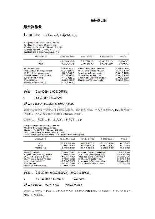
统计学2班第六次作业1、⑴①模型一：t t t PDI A A PCE μ++=21tt PDI E C P 008106.14269.216ˆ+-= t （-6.619723）（67.05920）996455.02=R F=4496.936 DW=1.366654美国个人消费支出受个人可支配收入影响，通过回归可知，个人可支配收入PDI 每增加一个单位，个人消费支出平均增加1.008106个单位。

②模型二：t t t t PCE B PDI B B PCE υ+++=-13211037158.0982382.02736.233ˆ-++-=t t t PCE PDI E C P T （-5.120436）（6.970817） （0.257997）996542.02=R F=2017.064 DW=1.570195美国个人消费支出PCE 不仅受当期个人可支配收入PDI 影响，还受滞后一期个人消费支出PCE t-1自身影响。

⑵从模型一得MPC=1.008106从模型二可得短期MPC=0.982382.从库伊特模型)()1(110---+++-=t t t t t Y X Y λμμλβλα可得1-t PEC 为λ的系数即037158.0=λ因为，长期MPC 即长期乘数为：∑=si iβ，根据库伊特模型)10(0<<=λλββii ，。

当s →∞时，λβλλβλβλβλβββββ-=--==+++=++=∞∞=∞=∑∑111 (00)102210100i ii i 所以长期MPC=02023.1037158.01982382.0=-=MPC2、Y ：固定资产投资 X ：销售额⑴ 设定模型为：t t t X Y μβα++=*，*t Y 为被解释变量的预期最佳值运用局部调整假定，模型转换为：*1*1*0*t t t t Y X Y μββα+++=- 其中：t t δμμδβδββδαα=-===**1*0*,1,,1271676.0629273.010403.15ˆ-++-=t t t Y X Y T （-3.193613） （6.433031） （2.365315）987125.02=R F=690.0561 DW=1.518595t t δμμδβδββδαα=-===**1*0*,1,, ，728324.0271676.011*1=-=-=βδ7381.20728324.010403.15*-=-==δαα，864.0728324.0629273.0*0===δββ∴局部调整模型估计结果为：tt X Y 864.07381.20ˆ*+-= 经济意义：该地区销售额每增加1亿元，未来预期最佳新增固定资产投资为0.846亿元采用德宾h 检验如下0:,0:10≠=ρρH H29728.1114858.0*21121)21.5185951()ˆ(1)21(2*1=--=--=βnVar n d h 在显著性水平05.0=α下，查标准正态分布表得临界值96.1025.02==h h α,因此拒绝原假设96.129728.1025.0=<=h h ，因此接受原假设，说明自回归模型不存在一阶自相关。

练习题7.1参考解答（1）先用第一个模型回归，结果如下：22216.4269 1.008106 t=(-6.619723) (67.0592)R 0.996455 R 0.996233 DW=1.366654 F=4496.936PCE PDI =-+==利用第二个模型进行回归，结果如下：122233.27360.9823820.037158 t=(-5.120436) (6.970817) (0.257997)R 0.996542 R 0.996048 DW=1.570195 F=2017.064t t t PCE PDI PCE -=-++==（2)从模型一得到MPC=1.008106；从模型二得到，短期MPC=0.982382，长期MPC= 0.982382+(0.037158)=1.01954 练习题7.2参考答案（1）在局部调整假定下，先估计如下形式的一阶自回归模型：*1*1*0*t t t t u Y X Y +++=-ββα 估计结果如下：122ˆ15.104030.6292730.271676 se=(4.72945) (0.097819) (0.114858)t= (-3.193613) (6.433031) (2.365315)R =0.987125 R =0.985695 F=690.0561 DW=1.518595t t t Y X Y -=-++根据局部调整模型的参数关系，有****11 ttu u αδαβδββδδ===-=将上述估计结果代入得到： *1110.2716760.728324δβ=-=-=*20.738064ααδ==-*0.864001ββδ==故局部调整模型估计结果为：*ˆ20.7380640.864001ttYX =-+ 经济意义解释：该地区销售额每增加1亿元，未来预期最佳新增固定资产投资为0.864001亿元。

运用德宾h 检验一阶自相关：(121(1 1.34022d h =-=-⨯=在显著性水平05.0=α上，查标准正态分布表得临界值21.96h α=，由于21.3402 1.96h h α=<=，则接收原假设0=ρ，说明自回归模型不存在一阶自相关。

习题7.1 解释概念（1）分类变量 （2）定量变量 （3）虚拟变量 （ 4）虚拟变量陷阱 （5）交互项（6）结构不稳定 （7）经季节调整后的时间序列答：（1）分类变量：在回归模型中，我们对具有某种特征或条件的情形赋值1，不具有某种特征或条件的情形赋值0，这样便定义了一个变量D ：1,0,D ⎧=⎨⎩具有某种特征不具有某种特征我们称这样的变量为分类变量。

（2）具有数值特征的变量，如工资、工作年数、受教育年数等，这些变量就称为定量变量。

（3）在回归模型中，我们对具有某种特征或条件的情形赋值1，不具有某种特征或条件的情形赋值0，这样便定义了一个变量D ：1,0,D ⎧=⎨⎩具有某种特征不具有某种特征 我们称这样的变量为虚拟变量（dummy variable ）。

（4）虚拟变量陷阱是指回归方程包含了所有类别（特征）对应的虚拟变量以及截距项，从而导致了完全共线性问题。

（5）交互项是指虚拟变量与定量变量相乘，或者两个定量变量相乘或是两个虚拟变量相乘，甚至更复杂的形式。

比如模型：12345i i i i i i i household lwage female married female married u βββββ=++++⋅+female married ⋅就是交互项。

（6）如果利用不同的样本数据估计同一形式的计量模型，可能会得到1β、2β不同的估计结果。

如果估计的参数之间存在着显著性差异，就称为模型结构不稳定。

（7）一些重要的经济时间序列，如果是受到季节性因素影响的数据，利用季节虚拟变量或者其他方法将其中的季节成分去除，这一过程被称为经季节调整的时间序列。

7.2 如果你有连续几年的月度数据，为检验以下假设，需要引入多少个虚拟变量？如何设定这些虚拟变量？（1）一年中的每一个月份都表现出受季节因素影响；（2）只有2、7、8月表现出受季节因素影响。

答：（1）对于一年中的每个月份都受季节因素影响这一假设，需要引入三个虚拟变量。

统计学2班第六次作业1、⑴①模型一：t t t PDI A A PCE μ++=21t tPDI E C P 008106.14269.216ˆ+-= t （-6.619723）（67.05920）996455.02=R F=4496.936 DW=1.366654美国个人消费支出受个人可支配收入影响，通过回归可知，个人可支配收入PDI 每增加一个单位，个人消费支出平均增加1.008106个单位。

②模型二：t t t t PCE B PDI B B PCE υ+++=-13211037158.0982382.02736.233ˆ-++-=t t tPCE PDI E C P T （-5.120436）（6.970817） （0.257997）996542.02=R F=2017.064 DW=1.570195美国个人消费支出PCE 不仅受当期个人可支配收入PDI 影响，还受滞后一期个人消费支出PCE t-1自身影响。

⑵从模型一得MPC=1.008106从模型二可得短期MPC=0.982382.从库伊特模型)()1(110---+++-=t t t t t Y X Y λμμλβλα可得1-t P E C 为λ的系数即037158.0=λ因为，长期MPC 即长期乘数为：∑=si iβ，根据库伊特模型)10(0<<=λλββi i ，。

当s →∞时，λβλλβλβλβλβββββ-=--==+++=++=∞∞=∞=∑∑111 (001)02210100i ii i所以长期MPC=02023.1037158.01982382.0=-=MPC2、Y ：固定资产投资 X ：销售额⑴ 设定模型为：t t t X Y μβα++=*，*t Y 为被解释变量的预期最佳值运用局部调整假定，模型转换为：*1*1*0*t t t t Y X Y μββα+++=- 其中：t t δμμδβδββδαα=-===**1*0*,1,,1271676.0629273.010403.15ˆ-++-=t t tY X Y T （-3.193613） （6.433031） （2.365315）987125.02=R F=690.0561 DW=1.518595t t δμμδβδββδαα=-===**1*0*,1,, ，728324.0271676.011*1=-=-=βδ7381.20728324.010403.15*-=-==δαα，864.0728324.0629273.0*0===δββ∴局部调整模型估计结果为：tt X Y 864.07381.20ˆ*+-= 经济意义：该地区销售额每增加1亿元，未来预期最佳新增固定资产投资为0.846亿元采用德宾h 检验如下0:,0:10≠=ρρH H29728.1114858.0*21121)21.5185951()ˆ(1)21(2*1=--=--=βnVar n d h 在显著性水平05.0=α下，查标准正态分布表得临界值96.1025.02==h h α,因此拒绝原假设96.129728.1025.0=<=h h ，因此接受原假设，说明自回归模型不存在一阶自相关。

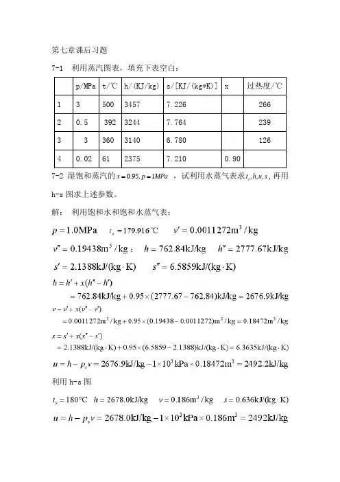
第七章课后习题7-1 利用蒸汽图表，填充下表空白：7-2 湿饱和蒸汽的0.95,1t h u s,再用x p MPa==，试利用水蒸气表求,,,sh-s图求上述参数。

解：利用饱和水和饱和水蒸气表：利用h-s图7-3 过程蒸汽的，试根据水蒸气表求,,,v h s u 和过热度，再用h-s 图求上述参数。

解：据水蒸气表，时、、利用 h-s 图。

7-4 已知水蒸气的压力0.5p MPa =、比体积30.35/v m kg =，问这是不是过热蒸汽？如果不是，那么是饱和蒸汽还是湿蒸汽？用水蒸气表求出其他参数。

解：利用水蒸气表时，，因所以该水蒸气不是过热蒸气而是饱和湿蒸汽。

据同一表查得：。

7-5 某锅炉每小时生产10 000kg 的蒸汽，蒸汽的表压力 1.9e p MPa = 、温度1350t C =︒。

设锅炉给水的温度240t C =︒，锅炉的效率0.78B η= ，煤的发热量（热值）42.9710/P Q KJ kg =⨯，求每小时锅炉的煤耗量是多少？锅炉内水的加热、汽化以及蒸汽的过热都在定压下进行。

锅炉效率 的定义为 B η=水和蒸汽所吸收的热量燃料燃烧时可提供的热量未被水和蒸汽吸收的热量是锅炉的热损失，其中主要是烟囱排烟带走的热能。

解：由查未饱和水和过热蒸汽表，得每生产 1kg 蒸汽需要吸入热量设每小时锅炉耗煤 mkg ，则7-6 1kg 113,450p MPa t C ==︒的蒸汽，可逆绝热膨胀至20.004p MPa =，试用h-s 图求终点状态参数2222,,,t v h s ，并求膨胀功w 和技术功t w 。

解：由 h-s 图查得：、、、。

膨胀功：技术功：7-7 1kg 、112,0.95p aMPa x ==的蒸汽，定温膨胀到21p MPa =，求终点状态参数2222,,,t v h s ，并求该过程中对蒸汽所加入的热量q 和过程中蒸汽对外界所作的膨胀功w. 解：由 h-s 图查得7-8 一台功率为20 000 KW 的汽轮机，其耗汽率61.3210/d kg J -=⨯。

计量经济学第七章第5,6,7题答案第7章练习5解：根据Eview 软件得如下表：Dependent Variable: YMethod: ML - Binary Logit (Quadratic hill climbing) Date: 05/22/11 Time: 22:19Sample: 1 16Included observations: 16Convergence achieved after 5 iterationsCovariance matrix computed using second derivativesVariableCoefficient Std. Error z-Statistic Prob.C -11.10741 6.124290 -1.813665 0.0697 Q 0.003968 0.008008 0.495515 0.6202 V0.0176960.0087522.0219140.0432 McFadden R-squared 0.468521 Mean dependent var 0.562500 S.D. dependent var 0.512348 S.E. of regression 0.382391 Akaike info criterion 1.103460 Sum squared resid 1.900896 Schwarz criterion 1.248321 Log likelihood-5.827681 Hannan-Quinn criter. 1.110878 Restr. loglikelihood -10.96503LR statistic 10.27469 Avg. log likelihood -0.364230Prob(LR statistic) 0.005873Obs with Dep=0 7 Total obs 16Obs with Dep=19于是，我们可得到Logit 模型为：V Q i0177.0004.0107.11Y ?++-= （-1.81）（0.49）（2.02）685.40R 2MCF = ， LR(2)=10.27如果在Binary estination 这⼀栏中选择Probit 估计⽅法，可得到如下表：Dependent Variable: YMethod: ML - Binary Probit (Quadratic hill climbing) Date: 05/22/11 Time: 22:25 Sample: 1 16Included observations: 16Convergence achieved after 5 iterationsCovariance matrix computed using second derivativesVariableCoefficient Std. Error z-Statistic Prob.C -6.634542 3.396882 -1.953127 0.0508 Q 0.002403 0.004585 0.524121 0.6002 V0.0105320.0046932.2442990.0248 McFadden R-squared 0.476272 Mean dependent var 0.562500 S.D. dependent var 0.512348 S.E. of regression 0.381655 Akaike info criterion 1.092836 Sum squared resid 1.893588 Schwarz criterion 1.237696 Log likelihood-5.742687 Hannan-Quinn criter. 1.100254 Restr. loglikelihood -10.96503LR statistic 10.44468 Avg. log likelihood -0.358918Prob(LR statistic) 0.005395Obs with Dep=0 7 Total obs 16Obs with Dep=19于是，我们可得到Probit 模型为：V Q i0105.00024.035.66Y ?++-= （-1.95）（0.52）（2.24）763.40R 2MCF = ， LR(2)=10.44第7章练习6 下表列出了美国、加拿⼤、英国在1980~1999年的失业率Y 以及对制造业的补偿X 的相关数解：（1）根据Eview 软件操作得如下表：美国（US ）：Dependent Variable: Y Method: Least Squares Date: 05/22/11 Time: 22:38 Sample: 1980 1999 Included observations: 20VariableCoefficientStd. Error t-Statistic Prob.C 10.56858 1.138982 9.278972 0.0000 X-0.0454030.012538-3.6211890.0020R-squared 0.421464 Mean dependent var 6.545000 Adjusted R-squared 0.389323 S.D. dependent var 1.432875 S.E. of regression 1.119732 Akaike infocriterion3.158696 Sum squared resid 22.56840 Schwarz criterion3.258269 Log likelihood -29.58696 Hannan-Quinncriter.3.178133 F-statistic 13.11301 Durbin-Watson stat 0.797022 Prob(F-statistic)0.001953根据上表可得对美国的OLS 估计结果为：tt X 0454.05686.10Y ?-= （9.28）（-3.62） 4215.02=R ， 3893.02=R ， D.W.=0.797， RSS=22.57加拿⼤(CA)：Dependent Variable: Y Method: Least Squares Date: 05/22/11 Time: 22:43Sample: 1980 1999 Included observations: 20。

第七章练习题及参考解答7.1 表7.4中给出了1981-2015年中国城镇居民人均年消费支出(PCE)和城镇居民人均可支配收入(PDI)数据。

表7.4 1981-2015年中国城镇居民消费支出(PCE)和可支配收入(PDI)数据 （单位：元）估计下列模型：tt t t tt t PCE B PDI B B PCE PDI A A PCE υμ+++=++=-132121(1) 解释这两个回归模型的结果。

(2) 短期和长期边际消费倾向（MPC ）是多少？分析该地区消费同收入的关系。

(3) 建立适当的分布滞后模型，用库伊克变换转换为库伊克模型后进行估计，并对估计结果进行分析判断。

【练习题7.1参考解答】(1) 解释这两个回归模型的结果。

Dependent Variable: PCE Method: Least Squares Date: 03/10/18 Time: 09:12 Sample: 1981 2005Variable Coefficient Std. Error t-Statistic Prob.C 149.0975 24.56734 6.068933 0.0000R-squared 0.998965 Mean dependent var 2983.768Adjusted R-squared 0.998920 S.D. dependent var 2364.412S.E. of regression 77.70773 Akaike info criterion 11.62040Sum squared resid 138885.3 Schwarz criterion 11.71791Log likelihood -143.2551 F-statistic 22196.24Durbin-Watson stat 0.531721 Prob(F-statistic) 0.000000收入跟消费间有显著关系。

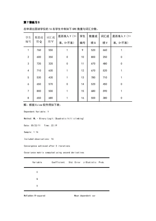
第7章练习5在申请出国读学位的16名学生中有如下GRE数量与词汇分数。

解：根据Eview软件得如下表：Dependent Variable: YMethod: ML - Binary Logit (Quadratic hill climbing)Date: 05/22/11 Time: 22:19Sample: 1 16Included observations: 16Convergence achieved after 5 iterationsCovariance matrix computed using second derivativesVariable Coefficient Std. Error z-Statistic Prob.CQVMcFadden R-squared Mean dependent var. dependent var . of regression Akaike info criterion Sum squared resid Schwarz criterionLog likelihoodHannan-Quinn criter. Restr. loglikelihoodLR statistic Avg. log likelihoodProb(LR statistic)Obs with Dep=0 7 Total obs 16Obs with Dep=19于是，我们可得到Logit 模型为：V Q i0177.0004.0107.11Y ˆ++-= （） （） （）685.40R 2MCF = ， LR(2)=如果在Binary estination 这一栏中选择Probit 估计方法，可得到如下表：Dependent Variable: YMethod: ML - Binary Probit (Quadratic hill climbing) Date: 05/22/11 Time: 22:25 Sample: 1 16Included observations: 16Convergence achieved after 5 iterationsCovariance matrix computed using second derivativesVariable Coefficient Std. Error z-Statistic Prob.C QVMcFadden R-squared Mean dependent var . dependent var . of regression Akaike info criterion Sum squared resid Schwarz criterionLog likelihoodHannan-Quinn criter. Restr. loglikelihoodLR statistic Avg. log likelihoodProb(LR statistic)Obs with Dep=0 7 Total obs 16Obs with Dep=19于是，我们可得到Probit 模型为：V Q i0105.00024.035.66Y ˆ++-= （） （） （）763.40R 2MCF = ， LR(2)=第7章练习6下表列出了美国、加拿大、英国在1980~1999年的失业率Y 以及对制造业的补偿X 的相关数据资料。

CHAPTER 7Exercise Solutions141Chapter 7, Exercise Solutions, Principles of Econometrics, 3e 142EXERCISE 7.1(a) When a GPA is increased by one unit, and other variables are held constant, averagestarting salary will increase by the amount $1643 ( 4.66t =, and the coefficient is significant at α = 0.001). Students who take econometrics will have a starting salary which is $5033 higher, on average, than the starting salary of those who did not take econometrics (11.03t =, and the coefficient is significant at α = 0.001). The intercept suggests the starting salary for someone with a zero GPA and who did not take econometrics is $24,200. However, this figure is likely to be unreliable since there would be no one with a zero GPA . The R 2 = 0.74 implies 74% of the variation of starting salary is explained by GPA and METRICS(b) A suitably modified equation is 1234SAL GPA METRICS FEMALE e =β+β+β+β+ Then, the parameter 4β is an intercept dummy variable that captures the effect of genderon starting salary, all else held constant.()()1231423if = 0if = 1GPA METRICSFEMALE E SAL GPA METRICS FEMALE β+β+β⎧⎪=⎨β+β+β+β⎪⎩(c) To see if the value of econometrics is the same for men and women, we change the modelto 12345SAL GPA METRICS FEMALE METRICS FEMALE e =β+β+β+β+β×+ Then, the parameter 4β is an intercept dummy variable that captures the effect of genderon starting salary, all else held constant. The parameter 5β is a slope dummy variable that captures any change in the slope for females, relative to males.()()()12314235if = 0if = 1GPA METRICSFEMALE E SAL GPA METRICS FEMALE β+β+β⎧⎪=⎨β+β+β+β+β⎪⎩Chapter 7, Exercise Solutions, Principles of Econometrics, 3e 143EXERCISE 7.2(a) Considering each of the coefficients in turn, we have the following interpretations.Intercept : At the beginning of the time period over which observations were taken, on a day which is not Friday, Saturday or a holiday, and a day which has neither a full moon nor a half moon, the estimated average number of emergency room cases was 93.69.T : We estimate that the average number of emergency room cases has been increasing by 0.0338 per day, other factors held constant. This time trend has a t -value of 3.058 and a p -value = 0.0025 < 0.01.HOLIDAY : The average number of emergency room cases is estimated to go up by 13.86on holidays. The “holiday effect” is significant at the 0.05 level of significance. FRI and SAT : The average number of emergency room cases is estimated to go up by 6.9and 10.6 on Fridays and Saturdays, respectively. These estimated coefficients are both significant at the 0.01 level. FULLMOON : The average number of emergency room cases is estimated to go up by2.45 on days when there is a full moon. However, a null hypothesis stating that a full moon has no influence on the number of emergency room cases would not be rejected at any reasonable level of significance. NEWMOON : The average number of emergency room cases is estimated to go up by 6.4on days when there is a new moon. However, a null hypothesis stating that a new moon has no influence on the number of emergency room cases would not be rejected at the usual 10% level, or smaller. Therefore, hospitals should expect more calls on holidays, Fridays and Saturdays, and also should expect a steady increase over time.(b)There are very little changes in the remaining coefficients, or their standard errors, when FULLMOON and NEWMOON are omitted. The equation goodness-of-fit statistic decreases slightly, as expected when variables are omitted. Based on these casual observations the consequences of omitting FULLMOON and NEWMOON are negligible. (c) The null and alternative hypotheses are067:0H β=β= 167: or is nonzero.H ββThe test statistic is()2(2297)R U U SSE SSE F SSE −=−whereR SSE = 27424.19 is the sum of squared errors from the estimated equation with FULLMOON and NEWMOON omitted and U SSE = 27108.82 is the sum of squared errors from the estimated equation with these variables included. The calculated value of the F statistic is 1.29. The .05 critical value is (0.95,2,222) 3.307F =, and corresponding p -value is0.277. Thus, we do not reject the null hypothesis that new and full moons have no impact on the number of emergency room cases.Chapter 7, Exercise Solutions, Principles of Econometrics, 3e 144EXERCISE 7.3(a) The estimated coefficient of the price of alcohol suggests that, if the price of pure alcohol goes up by $1 per liter, the average number of days (out of 31) that alcohol is consumed will fall by 0.045.(b) The price elasticity at the means is given by24.780.0450.3203.49q pp q∂=−×=−∂(c) To compute this elasticity, we need q for married black males in the 21-30 age range. It is given by4.0990.04524.780.00005712425 1.6370.8070.0350.5803.97713q =−×+×+−+−=Thus, the price elasticity is24.780.0450.2803.97713q p p q ∂=−×=−∂ (d)The coefficient of income suggests that a $1 increase in income will increase the averagenumber of days on which alcohol is consumed by 0.000057. If income was measured in terms of thousand-dollar units, which would be a sensible thing to do, the estimated coefficient would change to 0.057.(e) The effect of GENDER suggests that, on average, males consume alcohol on 1.637 moredays than women. On average, married people consume alcohol on 0.807 less days than single people. Those in the 12-20 age range consume alcohol on 1.531 less days than those who are over 30. Those in the 21-30 age range consume alcohol on 0.035 more days than those who are over 30. This last estimate is not significantly different from zero, however. Thus, two age ranges instead of three (12-20 and an omitted category of more than 20), are likely to be adequate. Black and Hispanic individuals consume alcohol on 0.580 and 0.564 less days, respectively, than individuals from other races. Keeping in mind that the critical t -value is 1.960, all coefficients are significantly different from zero, except that for the dummy variable for the 21-30 age range.Chapter 7, Exercise Solutions, Principles of Econometrics, 3e 145EXERCISE 7.4(a) The estimated coefficient for SQFT suggests that an additional square foot of floor spacewill increase the price of the house by $72.79. The positive sign is as expected, and the estimated coefficient is significantly different from zero. The estimated coefficient for AGE implies the house price is $179 less for each year the house is older. The negative sign implies older houses cost less, other things being equal. The coefficient is significantly different from zero.(b) The estimated coefficients for the dummy variables are all negative and they becomeincreasingly negative as we move from D92 to D96. Thus, house prices have been steadily declining in Stockton over the period 1991-96, holding constant both the size and age of the house.(c) Including a dummy variable for 1991 would have introduced exact collinearity unless theintercept was omitted. Exact collinearity would cause least squares estimation to fail. The collinearity arises between the dummy variables and the constant term because the sum of the dummy variables equals 1; the value of the constant term.Chapter 7, Exercise Solutions, Principles of Econometrics, 3e 146EXERCISE 7.5(a)The estimated marginal response of yield to nitrogen is()()8.0112 1.9440.5677.444 3.888when 16.877 3.888when 26.310 3.888when 3E YIELD NITRO PHOS NITRO NITRO PHOS NITRO PHOS NITROPHOS ∂=−××−×∂=−==−==−=The effect of additional nitrogen on yield depends on both the level of nitrogen and the level of phosphorus. For a given level of phosphorus, marginal yield is positive for small values of NITRO but becomes negative if too much nitrogen is applied. The level of NITRO that achieves maximum yield for a given level of PHOS is obtained by setting the first derivative equal to zero. For example, when PHOS = 1 the maximum yield occurs when NITRO = 7.444/3.888 = 1.915. The larger the amount of phosphorus used, the smaller the amount of nitrogen required to attain the maximum yield. (b)The estimated marginal response of yield to phosphorous is()()4.80020.7780.5674.233 1.556when 13.666 1.556when 23.099 1.556when 3E YIELD PHOS NITRO PHOS PHOS NITRO PHOS NITRO PHOSNITRO ∂=−××−×∂=−==−==−= Comments similar to those made for part (a) are also relevant here.(c)(i) We want to test 0246:20H β+β+β= against the alternative 1246:20.H β+β+β≠The value of the test statistic is ()24624627.367se 2b b b t b b b ++===++At a 5% significance level, the critical t -value is c t ± where (0.975,21) 2.080c t t ==. Since t > 2.080 we reject the null hypothesis and conclude that the marginal product ofyield to nitrogen is not zero when NITRO = 1 and PHOS = 1.(ii) We want to test 0246:40H β+β+β= against the alternative 1246:40H β+β+β≠.The value of the test statistic is()2462464 1.660se 4b b b t b b b ++===−++Since |t| < 2.080 (0.975,21)t =, we do not reject the null hypothesis. A zero marginal yieldwith respect to nitrogen is compatible with the data when NITRO = 1 and PHOS = 2.Chapter 7, Exercise Solutions, Principles of Econometrics, 3e 147Exercise 7.5(c) (continued)(c)(iii) We want to test 0246:60H β+β+β= against the alternative 1246:60H β+β+β≠.The value of the test statistic is()24624668.742se 6b b b t b b b ++===−++Since |t| > 2.080 (0.975,21)t =, we reject the null hypothesis and conclude that themarginal product of yield to nitrogen is not zero when NITRO = 3 and PHOS = 1.(d) The maximizing levels NITRO ∗ and PHOS ∗ are those values for NITRO and PHOS suchthat the first-order partial derivatives are equal to zero.()()35620E YIELD PHOS NITRO PHOS ∗∗∂=β+β+β=∂()()24620E YIELD NITRO PHOS NITRO ∗∗∂=β+β+β=∂The solutions and their estimates are 253622645228.011(0.778) 4.800(0.567)1.7014(0.567)4( 1.944)(0.778)NITRO ∗ββ−ββ××−−×−===β−ββ−−×−−34262264522 4.800( 1.944)8.011(0.567)2.4654(0.567)4( 1.944)(0.778)PHOS ∗ββ−ββ××−−×−===β−ββ−−×−−The yield maximizing levels of fertilizer are not necessarily the optimal levels. Theoptimal levels are those where the marginal cost of the inputs is equal to the marginal value product of those inputs. Thus, the optimal levels are those for which()()PHOS PEANUTS E YIELD PRICE PHOS PRICE ∂=∂ and ()()NITROPEANUTSE YIELD PRICE NITRO PRICE ∂=∂Chapter 7, Exercise Solutions, Principles of Econometrics, 3e 148EXERCISE 7.6(a) The model to estimate is()()112323ln +PRICE UTOWN SQFT SQFT UTOWN AGE POOL FPLACE e=β+δ+β+γ×β+δ+δ+The estimated equation, with standard errors in parentheses, isn ()()()()()()ln 4.46380.33340.035960.003428(se)0.02640.03590.001040.001414PRICE UTOWN SQFT SQFT UTOWN =++−×()()()20.0009040.018990.0065560.86190.0002180.005100.004140AGE POOL FPLACER −++=(b) In the log-linear functional form 12ln(),y x e =β+β+ we have21dy dx y=β or 2dydx y =β Thus, a 1 unit change in x leads to a percentage change in y equal to 2100×β.In this case2311PRICE UTOWNSQFT PRICE PRICE AGE PRICE∂=β+γ∂∂=β∂Using this result for the coefficients of SQFT and AGE , we find that an additional 100 square feet of floor space increases price by 3.6% for a house not in University town; a house which is a year older leads to a reduction in price of 0.0904%. Both estimated coefficients are significantly different from zero. (c) Using the results in Section 7.5.1a,()2ln()ln()100100%poolnopool PRICEPRICE PRICE −×=δ×≈Δan approximation of the percentage change in price due to the presence of a pool is 1.90%. Using the results in Section7.5.1b,()21001100pool nopool nopool PRICE PRICE e PRICE δ⎛⎞−×=−×⎜⎟⎜⎟⎝⎠the exact percentage change in price due to the presence of a pool is 1.92%.Chapter 7, Exercise Solutions, Principles of Econometrics, 3e 149Exercise 7.6 (continued)(d) From Section 7.5.1a,()3ln()ln()100100%fireplacenofireplace PRICEPRICE PRICE −×=δ×≈Δan approximation of the percentage change in price due to the presence of a fireplace is 0.66%.From Section 7.5.1b,()31001100fireplace nofireplace nofireplace PRICE PRICE e PRICE δ⎛⎞−×=−×⎜⎟⎜⎟⎝⎠the exact percentage change in price due to the presence of a fireplace is also 0.66%. (e)In this case the difference in log-prices is given by()n ()n ()2525ln ln 0.33340.003428250.33340.003428250.2477utown noutown SQFT SQFT PRICE PRICE UTOWN UTOWN ==−=−××=−×= and the percentage change in price attributable to being near the university, for a 2500square-feet home, is()0.2477110028.11%e−×=Chapter 7, Exercise Solutions, Principles of Econometrics, 3e 150EXERCISE 7.7(a) The estimated equation isn ()()()()()()()2ln 8.9848 3.7463 1.1495 1.2880.4237 (se)0.64640.57650.44860.60530.1052 1.4313 0.84280.1562SAL1APR1APR2APR3DISP DISPAD R =−++++=(b) The estimates of2β, 3β and 4β are all significant and have the expected signs. The sign of 2β is negative, while the signs of the other two coefficients are positive. These signs imply that Brands 2 and 3 are substitutes for Brand 1. If the price of Brand 1 rises, then sales of Brand 1 will fall, but a price rise for Brand 2 or 3 will increase sales of Brand 1. Furthermore, with the log-linear function, the coefficients are interpreted as proportionalchanges in quantity from a 1-unit change in price. For example, a one-unit increase in the price of Brand 1 will lead to a 375% decline in sales; a one-unit increase in the price of Brand 2 will lead to a 115% increase in sales. These percentages are large because prices are measured in dollar units. If we wish toconsider a 1 cent change in price – a change more realistic than a 1-dollar change – then the percentages 375 and 115 become 3.75% and 1.15%, respectively. (c) There are three situations that are of interest. (i) No display and no advertisement{}11234exp SAL1APR1APR2APR3Q =β+β+β+β=(ii) A display but no advertisement{}{}2123455exp exp SAL1APR1APR2APR3Q =β+β+β+β+β=β(iii) A display and an advertisement{}{}3123466exp exp SAL1APR1APR2APR3Q =β+β+β+β+β=βThe estimated percentage increase in sales from a display but no advertisement isn n n 210.423751exp{}100100(1)10052.8%Q b Q SAL1SAL1e Q SAL1−−×=×=−×=Chapter 7, Exercise Solutions, Principles of Econometrics, 3e 151Exercise 7.7(c) (continued)(c) The estimated percentage increase in sales from a display and an advertisement isn n n 311.431361exp{}100100(1)100318%Q b Q SAL1SAL1e Q SAL1−−×=×=−×=The signs and relative magnitudes of 5b and 6b lead to results consistent with economiclogic. A display increases sales; a display and an advertisement increase sales by an even larger amount.(d) The results of these tests appear in the table below.Part 0H Test Value Degrees of Freedom 5% Critical ValueDecision(i) β5 = 0 t = 4.03 46 2.01 Reject H 0 (ii) β6 = 0 t = 9.17 46 2.01 Reject H 0 (iii) β5 = β6 = 0 F = 42.0 (2,46) 3.20 Reject H 0 (iv)β6 ≤ β5t = 6.8646 1.68 Reject H 0(e) The test results suggest that both a store display and a newspaper advertisement will increase sales, and that both forms of advertising will increase sales by more than a store display by itself.Chapter 7, Exercise Solutions, Principles of Econometrics, 3e 152EXERCISE 7.8(a) The estimated equation, with standard errors in parentheses, isn 215.45970.2698 2.35820.4391(se) (0.2537)(0.0868)(0.2629)PRICEAGE NET R =+−=All estimated coefficients are significantly different from zero. The intercept suggests thatthe average price of CDs that have a 1999 copyright and are not sold on the internet is $15.46. For every year the copyright date is earlier than 1999, the price increases by 27 cents. For CDs sold through the internet, the price is $2.36 cheaper. The positive coefficient of AGE supports Mixon and Ressler’s hypothesis. (b) The estimated equation, with standard errors in parentheses, isn 215.52880.7885 2.35690.4380(se) (0.2424)(0.2567) (0.2632)PRICEOLD NET R =+−=Again, all estimated coefficients are significantly different from zero. They suggest thatthe average price of new releases, not sold on the internet, is $15.53. If the CD is not a new release, the price is 79 cents higher. If it is purchased over the internet, the price is $2.36 less. The positive coefficient of OLD supports Mixon and Ressler’s hypothesis.Chapter 7, Exercise Solutions, Principles of Econometrics, 3e 153EXERCISE 7.9The estimated coefficients and their standard errors (in parenthesis) for the various parts ofthis question are given in the following table.Variable (a) (b) (c) (f) (g) Constant (β1) 128.98* 342.88* 161.47 109.72 98.48(34.59) (72.34) (120.7) (135.6) (179.1)2()AGE β −7.5756* −2.9774 −2.0383 −1.7200 (2.317) (3.352) (3.542) (4.842) 3()INC β 1.4577* 2.3822* 9.0739* 18.325 22.104(0.5974) (0.6036) (3.670) (11.49) (40.26)4()AGE INC ×β −0.1602 −0.6115 −0.9087 (0.0867) (0.5381) (3.079)25()AGE INC ×β 0.0055 0.0131 (0.0064) (0.0784)36()AGE INC ×β −0.000065 (0.000663) SSE 819286 635637 580609 568869 568708 N K − 38 37 36 35 34* indicates a t -value greater than 2.(a) See table.(b) The signs of the estimated coefficients suggest that pizza consumption responds positivelyto income and negatively to age, as we would expect. All estimated coefficients are greater than twice their standard errors, indicating they are significantly different from zero using one or two-tailed tests. We note that scaling the income variable (dividing by 1000) has increased the coefficient 1000 times. (c) To comment on the signs we need to consider the marginal effects()()24E PIZZA INC AGE ∂=β+β∂()34E PIZZA AGE INC∂=β+β∂We expect β3 > 0 and β4 < 0 implying that the response of pizza consumption to incomewill be positive, but that it will decline with age. The estimates agree with these expectations. Negative signs for b 2 and b 4 imply that, as someone ages, his or her pizza consumption will decline, and the decline will be greater the higher the level of income.Chapter 7, Exercise Solutions, Principles of Econometrics, 3e 154Exercise 7.9(c) (continued)(c) The t value for the age-income interaction variable is t = −0.1602/0.0867 = −1.847.Critical values for a 5% significance level and one and two-tailed tests are, respectively, (0.05,36) 1.688t =− and (0.025,36) 2.028t =−. Thus, if we use the prior information β4 < 0, thenwe find the interaction coefficient is significant. However, if a two-tailed test is employed, the estimated coefficient is not significant. The coefficients of INC and (INC × AGE ) have increased 1000 times due to the effects of scaling.(d) The hypotheses areH 0: β2 = β4 = 0andH 1: β2 ≠ 0 and/or β4 ≠ 0The value of the F statistic under the assumption that H 0 is true is()()()81928658060927.4058060936R U U SSE SSE J F SSE T -K −−===The 5% critical value for (2, 36) degrees of freedom is F c = 3.26 and the p -value of the testis 0.002. Thus, we reject H 0 and conclude that age does affect pizza expenditure. (e) The marginal propensity to spend on pizza is given by()34E PIZZA AGE INC∂=β+β∂Point estimates, standard errors and 95% interval estimates for this quantity, for different ages, are given in the following table.Point Standard Confidence Interval AgeEstimate Error Lower Upper20 5.870 1.977 1.861 9.878 30 4.268 1.176 1.882 6.653 40 2.665 0.605 1.439 3.892 50 1.063 0.923 −0.8092.935The interval estimates were calculated using (0.975,36) 2.0281c t t ==. As an example of how the standard errors were calculated, consider age 30. We have()n ()n ()n ()n ()23434344var 30var 30var 230cov ,13.4669000.0075228600.31421 1.38392se 30 1.1763b b b b b b b b +=++×=+×−×=+==The corresponding interval estimate is4.268 ± 2.028 × 1.176 = (1.882, 6.653)Chapter 7, Exercise Solutions, Principles of Econometrics, 3e 155Exercise 7.9(e) (continued)(e)The point estimates for the marginal propensity to spend on pizza decline as age increases, as we would expect. However, the confidence intervals are relatively wide indicating that our information on the marginal propensities is not very reliable. Indeed, all the confidence intervals do overlap. (f) This model is given by212345+PIZZA INC AGE AGE INC AGE INC e =ββ+β+β×+β×+The marginal effect of income is now given by()2245+E PIZZA AGE AGE INC∂=β+ββ∂If this marginal effect is to increase with age, up to a point, and then decline, then β5 < 0. The sign of the estimated coefficient b 5 = 0.0055 did not agree with this anticipation. However, with a t value of t = 0.0055/0.0064 = 0.86, it is not significantly different from zero.(g)Two ways to check for collinearity are (i) to examine the simple correlations between each pair of variables in the regression, and (ii) to examine the R 2 values from auxiliary regressions where each explanatory variable is regressed on all other explanatory variables in the equation. In the tables below there are 3 simple correlations greater than 0.94 in part (f) and 5 in part (g). The number of auxiliary regressions with R 2s greater than 0.99 is 3 for part (f) and 4 for part (g). Thus, collinearity is potentially a problem. Examining the estimates and their standard errors confirms this fact. In both cases there are no t -values which are greater than 2 and hence no coefficients are significantly different from zero. None of the coefficients are reliably estimated. In general, including squared and cubed variables can lead to collinearity if there is inadequate variation in a variable.Simple CorrelationsAGE AGE INC ×2AGE INC × 3AGE INC ×INC 0.4685 0.9812 0.9436 0.8975 AGE0.5862 0.6504 0.6887 AGE INC × 0.9893 0.9636 2AGE INC ×0.9921R 2 Values from Auxiliary RegressionsLHS variableR 2 in part (f) R 2 in part (g)INC0.99796 0.99983 AGE0.68400 0.82598 AGE INC × 0.99956 0.99999 2AGE INC × 0.99859 0.999993AGE INC × 0.99994Chapter 7, Exercise Solutions, Principles of Econometrics, 3e 156EXERCISE 7.10(a) The estimated equation with gender (FEMALE ) included, and with standard errors written in parentheses, isn ()()()()461.86408.18280.0024190.2581 (se)51.3441 1.55010.000427.7681PIZZA AGE INCOME FEMALE =−+−The t -value for gender is 190.258127.7681 6.8517t =−=− indicating that it is a relevantexplanatory variable. Including it in the model has led to substantial changes in the coefficients of the remaining variables.(b) When level of educational attainment is included the estimated model, with the standarderrors in parentheses, becomesn ()()()()317.38988.30140.002990.7944 (se)83.3909 2.32630.000757.8402PIZZAAGE INCOME HS =−++()()1.680273.204762.662192.0859COLLEGE GRAD−−None of the dummy variable coefficients are significant, casting doubt on the relevance of education as an explanatory variable. Also, including the education dummies has had little impact on the remaining coefficient estimates. To confirm the lack of evidence supporting the inclusion of education, we need to use an F test to jointly test whether the coefficients of HS, COLLEGE and GRAD are all zero. The value of this statistic is()()()63563753944632.020*********R U U SSE SSE J F SSE N K −−===−The 5% critical value for (3, 34) degrees of freedom is F c = 3.05; the p -value is 0.13. Wecannot conclude that level of educational attainment influences pizza consumption. (c) To test this hypothesis we estimate a model where the dummy variable gender (FEMALE ) interacts with every other variable in the equation. The estimated equation, with standard errors in parentheses, isn ()()()()451.36059.36320.0036208.3393 (se)63.9450 1.91550.000796.5078PIZZA AGE INCOME FEMALE =−+−()()2.83370.00183.08710.0008AGE×FEMALE INCOME×FEMALE−Chapter 7, Exercise Solutions, Principles of Econometrics, 3e 157Exercise 7.10(c) (continued)(c)To test the hypothesis that the regression equations for males and females are identical, we test jointly whether the coefficients of FEMALE , AGE ×FEMALE , INCOME ×FEMALE are all zero. Note that individual t tests on each of these coefficients do not suggest gender is relevant. However, when we take all variables together, the F value for jointly testing their coefficients is()()()635636.7244466.5318.1344244466.534R U U SSE SSE J F SSE N K −−===−This value is greater than F c = 2.866 which is the 5% critical value for (3, 36) degrees offreedom. The p -value is 0.0000. Thus, we reject the null hypothesis that males and females have identical pizza expenditure equations. This result implies different equations should be used to model pizza expenditure for males, and that for females. It does not say how the equations differ. For example, all their coefficients could be different, or simply modelling different intercepts might be adequate.Chapter 7, Exercise Solutions, Principles of Econometrics, 3e 158EXERCISE 7.11(a) The estimated result, with standard errors in parentheses, isn ()()()()161.4654 2.97740.009070.00016(se)120.6634 3.35210.003670.0000867PIZZA AGE INCOME INCOME×AGE =−+−This is identical to the result reported in 7.4.(b) From the sample we obtain average age = 33.475 and average income = 42,925. Thus, the required marginal effect of income isn ()0.009070.0001633.4750.00371E PIZZA INCOME∂=−×=∂Using computer software, we find the standard error of this estimate to be 0.000927, and the t value for testing whether the marginal effect is significantly different from zero is t =0.003710.000927 4.00=. The corresponding p -value is 0.0003 leading us to conclude that the marginal income effect is statistically significant at a 1% level of significance.(c) A 95% interval estimate for the marginal income effect is given by0.00371 ± 2.0281 × 0.000927 = (0.00183, 0.00559)(d) The marginal effect of age for an individual of average income is given byn ()()E PIZZA AGE ∂∂= −2.9774 − 0.00016INCOME = −2.9774 − 0.00016 × 42,925 = −9.854 Using computer software, we find the standard error of this estimate to be 2.5616, and thet value for testing whether the marginal effect is significantly different from zero is 9.8542.5616 3.85t =−=−The p -value of the test is 0.0005, implying that the marginal age effect is significantlydifferent from zero at a 1% level of significance. (e) A 95% interval estimate for the marginal age effect is given by −9.854 ± 2.0281 × 2.5616 = (−15.05, −4.66)Chapter 7, Exercise Solutions, Principles of Econometrics, 3e 159Exercise 7.11 (continued)(f)Important pieces of information for Gutbusters are the responses of pizza consumption to age and income. It is helpful to know the demand for pizzas in young and old communities and in high and low income areas. A good starting point in an investigation of this kind is to evaluate the responses at average age and average income. Such an evaluation will indicate whether there are noticeable responses, and, if so, give some idea of their magnitudes. The two responses are estimated asn ()E PIZZA INCOME ∂∂ = 0.0037n ()()E PIZZA AGE ∂∂ = −9.85Both these estimates are significantly different from zero at a 1% level of significance. They suggest that increasing income will increase pizza consumption, but, as a community ages, its demand for pizza declines. Interval estimates give an indication of the reliability of the estimated responses. In this context, we estimate that the income response lies between 0.0018 and 0.0056, while the age response lies between −15.05 and −4.66.。