5外文翻译原文

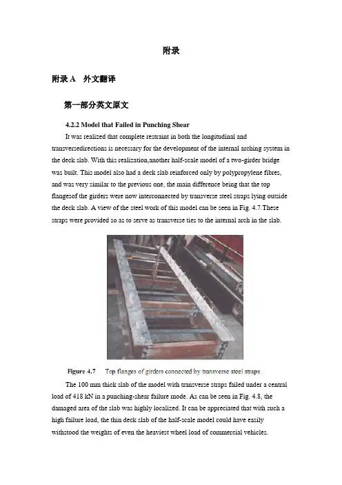
附录附录A 外文翻译第一部分英文原文4.2.2 Model that Failed in Punching ShearIt was realized that complete restraint in both the longitudinal and transversedirections is necessary for the development of the internal arching system in the deck slab. With this realization,another half-scale model of a two-girder bridge was built. This model also had a deck slab reinforced only by polypropylene fibres, and was very similar to the previous one, the main difference being that the top flangesof the girders were now interconnected by transverse steel straps lying outside the deck slab. A view of the steel work of this model can be seen in Fig. 4.7.These straps were provided so as to serve as transverse ties to the internal arch in the slab.The 100 mm thick slab of the model with transverse straps failed under a central load of 418 kN in a punching-shear failure mode. As can be seen in Fig. 4.8, the damaged area of the slab was highly localized. It can be appreciated that with such a high failure load, the thin deck slab of the half-scale model could have easily withstood the weights of even the heaviest wheel load of commercial vehicles.The model tests described above and in sub-section 4.2.1 clearly demonstrate that an internal arching action will indeed develop in a deck slab, but only if it is suitably restrained.4.2.3 Edge StiffeningA further appreciation of the deck slab arching action is provided by tests on a scale model of a skew slab-on-girder bridge. As will be discussed in sub-section 4.4.2, one transverse free edge of the deck slab of this model was stiffened by a composite steel channel with its web in the vertical plane. The other free edge was stiffened by a steel channel diaphragm with its web horizontal and connected to the deck slab through shear connectors. The deck slab near the former transverse edge failed in a mode that was a hybrid between punching shear and flexure. Tests near the composite diaphragm led to failure at a much higher load in punching shear (Bakht and Agarwal, 1993).The above tests confirmed yet again that the presence of the internal arching action in deck slabs induces high in-plane force effects which in turn demand stiffer restraint in the plane of the deck than in the out-of-plane direction.4.3 INTERNALLY RESTRAINED DECK SLABSDeck slabs which require embedded reinforcement for strength will now be referred to as internally restrained deck slabs. The state-of-art up to 1986 relating to the quantification and utilization of the beneficial internal arching action in deck slabs with steel reinforcement has been provided by Bakht and Markovic (1986). Their conclusions complemented with up-to-date information are presented in this chapter in a generally chronological order which, however, cannot be adhered to rigidlybecause of the simultaneous occurrence of some developments.4.3.1 Static Tests on Scale ModelsAbout three decades ago, the Structures Research Office of the Ministry of Transportation of Ontario (MTO), Canada, sponsored an extensive laboratory-based research program into the load carrying capacity of deck slabs; this research program was carried out at Queen's University, Kingston, Ontario. Most of this research was conducted through static tests on scale models of slab-on-girder bridges. This pioneering work is reported by Hewitt and Batchelor (1975) and later by Batchelor et al. (1985), and is summarized in the following.The inability of the concrete to sustain tensile strains, which leads to cracking, has been shown to be the main attribute which causes the compressive membrane forces to develop. This phenomenon is illustrated in Fig. 4.9 (a) which shows the part cross-section of slab-on-girder bridge under the action of a concentrated load.The cracking of the concrete, as shown in the figure, results in a net compressive force near the bottom face of the slab at each of the two girder locations. Midway between the girders, the net compressive force moves towards the top of the slab. It can be readily visualized that the transition of the net compressive force from near the top in the middle region, to near the bottom at the supports corresponds to the familiar arching action. Because of this internal arching action, the failure mode of a deck slab under a concentrated load becomes that of punching shear.If the material of the deck slab has the same stress-strain characteristics in both tension and compression, the slab will not crack and, as shown in Fig. 4.9 (b), will not develop the net compressive force and hence the arching action.In the punching shear type of failure, a frustum separates from the rest of the slab, as shown in schematically in Fig. 4.10. It is noted that in most failure tests, the diameter of the lower end of the frustrum extends to the vicinity of the girders.From analytical and confirmatory laboratory studies, it was established that the most significant factor influencing the failure load of a concrete deck slab is the confinement of the panel under consideration. It was concluded that this confinement is provided by the expanse of the slab beyond the loaded area; its degree was founddifficult to assess analytically. A restraint factor, η, was used as an empirical measure of the confinement; its value is equal to zero for the case of no confinement and 1.0 for full confinement.The effect of various parameters on the failure load can be seen in Table 4.1, which lists the theoretical failure loads for various cases. It can be seen that an increase of the restraint factor from 0.0 to 0.5 results in a very large increase in the failure load. The table also emphasizes the fact that neglect of the restraint factor causes a gross underestimation of the failure load.It was concluded that design for flexure leads to the inclusion of large amounts of unnecessary steel reinforcement in the deck slabs, and that even the minimum amount of steel required for crack control against volumetric changes in concrete is adequate to sustain modern-day, and even future, highway vehicles of North America.It was recommended that for new construction, the reinforcement in a deck slab should be in two layers, with each layer consisting of an orthogonal mesh having the same area of reinforcement in each direction. The area of steel reinforcement in each direction of a mesh was suggested to be 0.2% of the effective area of cross-section of the slab. This empirical method of design was recommended for deck slabs with certain constraints.4.3.2 Pulsating Load Tests on Scale ModelsTo study the fatigue strength of deck slabs with reduced reinforcement, five small scale models with different reinforcement ratios in different panels were tested at the Queen's University at Kingston. Details of this study are reported by Batchelor et al. (1978).Experimental investigation confirmed that for loads normally encountered in North America deck slabs with both conventional and recommended reducedreinforcement have large reserve strengths against failure by fatigue. It was confirmed that the reinforcement in the deck slab should be as noted in sub-section 4.3.1. It is recalled that the 0.2% reinforcement requires that the deck slab must have a minimum restraint factor of 0.5.The work of Okada, et al. (1978) also deals with fatigue tests on full scale models of deck slabs and segments of severely cracked slab removed from eight to ten year old bridges. The application of these test results to deck slabs of actual bridges is open to question because test specimens were removed from the original structures in such a way that they did not retain the confinement necessary for the development of the arching action.4.3.3 Field TestingAlong with the studies described in the preceding sub-section, a program of field testing of the deck slabs of in-service bridges was undertaken by the Structures Research Office of the MTO. The testing consisted of subjecting deck slabs to single concentrated loads, simulating wheel loads, and monitoring the load-deflection characteristics of the slab. The testing is reported by Csagoly et al. (1978) and details of the testing equipment are given by Bakht and Csagoly (1979).Values of the restraint factor, η, were back-calculated from measured deflections.A summary of test results, given in Table 4.2, shows that the average value of η in composite bridges is greater than 0.75, while that for non-composite bridges is 0.42. It was concluded that for new construction, the restraint factor, η, can be assumed to have a minimum value of 0.5.Bakht (1981) reports that after the first application of a test load of high magnitude on deck slabs of existing bridges, a small residual deflection was observed in most cases. Subsequent applications of the same load did not result in further residual deflections. It is postulated that the residual deflections are caused by cracking of the concrete which, as discussed earlier, accompanies the development of the internal arching action. The residual deflections after the first cycle of loading suggest that either the slab was never subjected to loads high enough to cause cracking, or the cracks have 'healed' with time.第二部分汉语翻译4.2.2 在冲切剪应力下的实效模型我们已经知道在桥面板内部拱形系统的形成中，不仅纵向而且横向也被完全约束限制是完全必要的。

外文翻译原文Foreign T rade o f ChinaMaterial Source:W anfang Database Author:Hitomi Iizaka1.IntroductionOn December11,2001,China officially joined the World T rade Organization(WTO)and be c a me its143rd member.China’s presence in the worl d economy will continue to grow and deepen.The foreign trade sector plays an important andmultifaceted role in China’s economic development.At the same time, China’s expanded role in the world economy is beneficial t o all its trading partners. Regions that trade with China benefit from cheaper and mor e varieties of imported consumer goods,raw materials and intermediate products.China is also a large and growing export market.While the entry of any major trading nation in the global trading system can create a process of adjustment,the o u t c o me is fundamentally a win-win situation.In this p aper we would like t o provide a survey of the various institutions,laws and characteristics of China’s trade.Among some of the findings, we can highlight thefollowing:•In2001,total trade to gross domestic pr oduct(GDP)ratio in China is44%•In2001,47%of Chinese trade is processed trade1•In2001,51%of Chinese trade is conduct ed by foreign firms in China2•In2001,36%of Chinese exports originate from Gu an gdon g province•In2001,39%of China’s exports go through Hong Kong to be re-exported elsewhere2.Evolution of China’s Trade RegimeEqually remarkable are the changes in the commodity composition of China’s exports and imports.Table2a shows China’s annu al export volumes of primary goods and manufactured goods over time.In1980,primary goods accounted for 50.3%of China’s exports and manufactured goods accounted for49.7%.Although the share of primary good declines slightly during the first half of1980’s,it remains at50.6%in1985.Since then,exports of manufactured goods have grown at a muchfaster rate than exports of primary goods.As a result,the share of manufactur ed goods increased t o90.1%,and that of primary good decr eased to9.9%by2001.Also shown in those tables are five subgr oups for manufactur ed goods and primary goods.China’s export was highly dependent on its exports of coal, petroleum,and petr oleum products until mid-80s.The large export volume of petr oleum was also support ed by a sharp rise in oil prices during the period.In1985, the share of mineral fuels is26.1%.In1986,the su d d en decline in the share of primary goods in total exports occurs,which is largely associated with the decline in the export volume of mineral fuels.The price reforms coupled with the declined world petr oleum price areattributable t o the decline.Domestic agriculture production expanded during the1980’s in response to the higher prices thr ough the price reforms and mo r e opportunities given t o the producers to market their products.Although the share of food and live animals in total exports has declined over time,China has become a net exporter of such products since1984.T urning to the manufactur ed goods,the large increase in the share of the manufactur ed goods in the total exports since mid-80s is largely accounted for by the increase in the export in the textile category and the miscellaneous products category.These two gr oups include labor-intensive products such as textiles,apparel, footwear,and toys and sporting goods.During the1990s,the category that exhibited the mos t significant surge in exports is machinery and transport equipment.Its share exp anded from9.0%in1990t o35.7%in2001.3.China’s Processing Trade and Trade by For eign Invested FirmsChina established the legal framework for processing and assembly arrangements in1979.Since then,China has built up considerable strengths in assembling and processing of industrial parts and components.It covers a wide range of industries such as electric machinery,automobile,aerospace,and shipbuilding.T able3a and T able3b demonstrate the amount of processing exports and imports and the importance of stateowned enterprises(SOEs)and foreign-invested enterprises(FIEs)in such forms of trade for1995-2001. Throughout the period from1995to2001,the shares of these two types of processing exports exceed more than half of China’s total exports.In2001，processing exports account for55.4%of the total exports.As is seen in T able3a, process&assembling was dominat ed by SOEs in1995.However,the tr end has been changing.The share of SOEs in process&assembling has been steadilydeclining over the years from84%in1995to62%in2001.The other type of trade, process with imported materials was largely conducted by FIEs and their shares have been gradually increasing from81%in1995to88%in2001.In China’s imports(see T able3b),processing trade is relatively small comp a r ed to exports. After it peak ed at49%in1997,processed imports decline to39%in2001.The decreasing importance of SOEs can be seen in China’s imports as well.Shares by SOEs decr eased from81%in1995t o58%in2001for process&assembling,and from18%to7%for process with imported materials.The decr eased role for SOEs in processing trade may reflect the inefficiency in conducting their business.Since 1997,the Chinese government decided t o implement the shareholding system and t o sell a large numbe r of medium-and small-sized SOEs to the private sector.A n u mbe r of larger enterprise gr oups will be established in various industries thr ough mergers,acquisitions,and leasing and contracting.The restructuring of SOEs is intended to increase profits and to improve their competitive edge.4.China’s Tr ade by Provinces and RegionsA regional breakdown of exports and imports reveals important characteristics of the foreign trade in China.In1997,89.1%of the total exports came from the Eastern region of China(Beijing,Tianjin,Heibei,Lioaning,Guangxi,Shanghai, Jiangsu,Zhejiang,Fujian,Shangdong,Guandong and Hainan).Within the East,the Southeast region accounts for76.3%of China's exports in1997.4Gu ang dong alone pr oduces41.6%of the total exports for the sa me year.Such regional imbalances in exporting activities persist to the present day.In2001,Guandong's share of the national exports is36.0%.For the Southeast and the East,the shares are respectively 79.0%and91.1%.This imbalance of the regional growth in foreign trade may partially be attributed t o the various geographic-specific and sequential o pen-d oo r policies China has exercised thr oughout the last twenty years.The strong growth of th e export sector in the coastal area has been support ed by the massive use of foreign direct investment(FDI).FDI was first attracted by the creation of the Special Economic Zones(SEZ).FDI was concentrated in the provinces of the Southeast coast,namely,Guandong and Fujian.The multinational enterprises that are export-oriented or use adv anced technologies are able to enjoy various preferential policies in the SEZs,such as r educed or ex empt e d corporate income tax,exemption from import tariffs on imported equipment and raw materials.In1984,fourteen coastal cities were opened and were grant ed similar policies as SEZs.Out of thosefourteen cities,ten are located in the Southeast coast regions and four are in the rest of the Eastern regions.Furthermore in1985,similar preferential policies were grant ed t o other coastal economic regions,Pearl River Delta,Y angtze River Delta and Minnan Delta which is t o the south of Fujian.In1990,Pu d o n g in Shanghai was opened and was grant ed extensive preferential policies.Since1984,the Chinese government established thirty-two national-level Economic and T echnological Development Zones(ETDZs).The share of exports in The Y angtze River Delta,the home of Shanghai and two provinces,Jiangsu and Zhejiang has grown steadily during the period1997to 2001.The share of those three regions grew to10.1%,11.0%,and9.1%in2001 from8.1%,7.9%and5.9%in1997,respectively.As the role of high-tech industry beco mes mo r e significant in China’s output and China’s comparative advantage in skilled-labor and capital-intensive industries beco mes higher,the Y angtze River Delta be co mes a new magnet for investment by foreign enterprises.These foreign investments in turn lead to mo r e export and trade.5.Foreign T rade by Major World RegionsUsing China’s official statistics,Table4a and4b highlight merchandise export s and imports t o and from major world regions for1993-2001:Asia,Africa,Europe, Latin America,North America and Oceania.As we see from Table4a,China’s most important export region has always been Asia,which absorbs53%of China’s exports in2001.However,their share of absorption declines from almost62%,their peak level of1995.The importance of North America and Europe in China’s exports, however,has been increasing since1998.In2001,North America takes in mo r e than22%of exports and Europe takes in mo r e than18%.6.China’s Merchandise Exports and Imports by Major Trading PartnersTable5a and Table5b document China’s merchandise exports to and imports from its major trading partners,using China’s official statistics.According to Tabl e 5a,the major exports markets for China in2001are:the United States(20.4%), Hong Kong(17.5%),Japan(16.9%)and the European Union(15.4%).It is well-known that a large proportion of Chinese exports to Hong Kong are re-exported elsewhere so that the true size of the Hong Kong export market has t o be estimated. T o save space for this paper,we will just rely on the official Chinese figures.6Even without adjusting for re-exports,the United States in2001is the largest export market for China.Thus,from an international trade perspective alone,the most important bilateral trade relationship for China is the relationship with the UnitedStates.T ogether t he United States,Hong Kong,Japan and the European Union take in70.2%of China’s exports in2001.Within ASEAN(Association of Southeast Asian Nations),Singapore has been the largest export market for China.In2001, 31.5%of China’s total exports to ASEAN is destined for Singapore.Within the European Union(EU),Germany is the largest market with23.8%of the total Chinese exports going to the EU.9.ConclusionIn the future,we see that there are at least two challenges facing China in the area of international trade.First,with China’s competitiveness growing,many countries will perceive that their producers will no t be able to c o mpe t e with the Chinese exports,either in the third market or in their own domestic market.The backlash will take the form of an increased use of anti-dumping duties and safeguards.W e have already seen the use of such trade instruments against China from a variety of countries,including Japan,the European Union and the United States.A relatively new development is that even developing countries such as India and Mexico are using anti-dumping measur es against Chinese exports to their countries.The difficulty with anti-dumping duties is that they are generally WT O-consistent.Thus joining the WTO d o es no t mean that other countries will reduce their use of anti-dumping duties against China.A second challenge facing China is how t o manage its trade relationship with the United States.The United States is the largest economy on earth.The United States is China’s largest export market.It is also a critical source of technology.A stable and healthy relationship with the United States is important for China’s economic development.It is always a difficult adjustment process for countries to accept a newly e mer gen t economic power.The United States as well as other countries may perceive China as a potential economic threat.Judging from the experience of the relationship betw een the United States and a rising Japan in the 1970s and the1980s,it will n o t be too har d to imagine that there will be difficulties in the trade relationship betw een the United States and China.Managing and smoothing such a relationship should be an important goal for China.译文中国的对外贸易资料来源:万方数据库作者：Hitomi Iizaka1、简介2001年12月11日，中国正式加入世界贸易组织（WTO），成为其第143个成员，中国在世界经济中的作用将继续增强和深化。

外文文献原稿和译文原稿logistics distribution center location factors:(1) the goods distribution and quantity. This is the distribution center and distribution of the object, such as goods source and the future of distribution, history and current and future forecast and development, etc. Distribution center should as far as possible and producer form in the area and distribution short optimization. The quantity of goods is along with the growth of the size distribution and constant growth. Goods higher growth rate, the more demand distribution center location is reasonable and reducing conveying process unnecessary waste.(2) transportation conditions. The location of logistics distribution center should be close to the transportation hub, and to form the logistics distribution center in the process of a proper nodes. In the conditional, distribution center should be as close to the railway station, port and highway.(3) land conditions. Logistics distribution center covers an area of land in increasingly expensive problem today is more and more important. Is the use of the existing land or land again? Land price? Whether to conform to the requirements of the plan for the government, and so on, in the construction distribution center have considered.(4) commodities flow. Enterprise production of consumer goods as the population shift and change, should according to enterprise's better distribution system positioning. Meanwhile, industrial products market will transfer change, in order to determine the raw materials and semi-finished products of commodities such as change of flow in the location of logistics distribution center should be considered when the flow of the specific conditions of the relevant goods.(5) other factors. Such as labor, transportation and service convenience degree, investment restrictions, etc.How to reduce logistics cost，enhance the adaptive capacity and strain capacity of distribution center is a key research question of agricultural product logistics distribution center．At present，most of the research on logistics cost concentrates off theoretical analysis of direct factors of logistics cost, and solves the problem of over-high logistics Cost mainly by direct channel solution．This research stresses on the view of how to loeate distribution center, analyzes the influence of locating distribution center on logistics cost．and finds one kind of simple and easy location method by carrying on the location analysis of distribution center through computer modeling and the application of Exeel．So the location of agricultural product logistics distribution center can be achieved scientifically and reasonably, which will attain the goal of reducing logistics cost, and have a decision．making support function to the logisties facilities and planning of agricultural product．The agricultural product logistics distribution center deals with dozens and even hundreds of clients every day, and transactions are made in high-frequency. If the distribution center is far away from other distribution points，the moving and transporting of materials and the collecting of operational data is inconvenient and costly. costly．The modernization of agricultural product logistics s distribution center is a complex engineering system，not only involves logistics technology, information technology, but also logistics management ideas and its methods，in particular the specifying of strategic location and business model is essential for the constructing of distribution center. How to reduce logistics cost，enhance the adaptive capacity and strain capacity of distribution center is a key research question of agricultural product logistics distribution center. The so—called logistics costs refers to the expenditure summation of manpower, material and financial resources in the moving process of the goods．such as loading and unloading，conveying，transport，storage，circulating，processing, information processing and other segments. In a word。

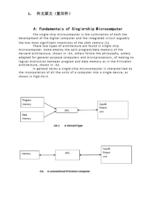
1、 外文原文（复印件）A: Fundamentals of Single-chip MicrocomputerT h e sin gle -ch ip mi c ro co m p u t e r is t h e cu lm in at io n of b ot h t h e d e ve lo p me nt of t h e d ig ita l co m p u t e r a n d t h e i nte g rated c ircu it a rgu ab l y t h e to w mo st s ign if i cant i nve nt i o n s of t h e 20t h c e nt u ry [1].T h ese to w t yp e s of arch ite ct u re are fo u n d in s in gle -ch ip m i cro co m p u te r. S o m e e mp l oy t h e sp l it p ro gra m /d at a m e m o r y of t h e H a r va rd arch ite ct u re , s h o wn in -5A , ot h e rs fo l lo w t h e p h i lo so p hy, wid e l y ad a p ted fo r ge n e ral -p u rp o se co m p u te rs an d m i cro p ro ce ss o rs , of m a kin g n o l o g i ca l d i st in ct i o n b et we e n p ro gra m an d d ata m e m o r y as in t h e P rin c eto n a rch ite ct u re , sh o wn in -5A.In ge n e ra l te r m s a s in g le -ch ip m ic ro co m p u t e r is ch a ra cte r ized b y t h e in co r p o rat io n of all t h e u n its of a co mp u te r into a s in gle d e vi ce , as s h o w n in F i g3-5A-3.-5A-1A Harvard type-5A. A conventional Princeton computerProgrammemory Datamemory CPU Input& Output unitmemoryCPU Input& Output unitResetInterruptsPowerFig3-5A-3. Principal features of a microcomputerRead only memory (ROM).RO M is u su a l l y fo r t h e p e r m an e nt , n o n -vo lat i le sto rage of an ap p l i cat io n s p ro g ram .M a ny m i c ro co m p u te rs a n d m i cro co nt ro l le rs are inte n d ed fo r h i gh -vo lu m e ap p l i cat io n s a n d h e n ce t h e e co n o m i cal man u fa c t u re of t h e d e vi ces re q u ires t h at t h e co nt e nts of t h e p ro gra m me mo r y b e co mm i ed p e r m a n e nt l y d u r in g t h e m a n u fa ct u re of c h ip s . C lea rl y, t h i s imp l ies a r i go ro u s ap p ro a ch to ROM co d e d e ve lo p m e nt s in ce ch an ges can n o t b e mad e af te r m an u fa ct u re .T h i s d e ve l o p m e nt p ro ces s m ay i nvo l ve e mu l at i o n u sin g a so p h ist icated d e ve lo p m e nt syste m wit h a h ard wa re e mu l at i o n capab i l it y as we ll as t h e u s e of p o we rf u l sof t war e to o l s.So m e m an u fa ct u re rs p ro vi d e ad d it i o n a l ROM o p t io n s b y in clu d in g in t h e i r ran ge d e v ic es w it h (o r inte n d ed fo r u s e wit h ) u se r p ro g ram m a b le m e mo r y. T h e s im p lest of t h e se i s u su a l l y d e v i ce wh i ch can o p e rat e in a m i cro p ro ce s so r mo d e b y u s in g s o m e of t h e in p u t /o u t p u t l in es as an ad d res s a n d d ata b u s fo r a cc es sin g exte rn a l m e m o r y. T h is t yp e o f d e vi ce can b e h ave f u n ct i o n al l y as t h e s in gle ch ip m i cro co m p u t e r f ro m wh i ch it i s d e ri ved a lb e it wit h re st r icted I/O an d a m o d if ied exte rn a l c ircu it. T h e u s e of t h e se RO M le ss d e vi ces i s co mmo n e ve n in p ro d u ct io n circu i ts wh e re t h e vo lu m e d o e s n ot ju st if y t h e d e ve lo p m e nt co sts of cu sto m o n -ch ip ROM [2];t h e re ca n st i ll b e a si gn if i cant sav in g in I/O an d o t h e r ch ip s co m pared to a External Timing components System clock Timer/ Counter Serial I/O Prarallel I/O RAM ROMCPUco nve nt io n al m i c ro p ro ces so r b ased circ u it. M o re exa ct re p l a ce m e nt fo rRO M d e v ice s can b e o b tain ed in t h e fo rm of va ria nts w it h 'p i g g y-b a c k'E P ROM(E rasab le p ro gramm ab le ROM )s o cket s o r d e v ice s w it h E P ROMin stead of ROM 。

5G无线通信网络中英文对照外文翻译文献(文档含英文原文和中文翻译)翻译：5G无线通信网络的蜂窝结构和关键技术摘要第四代无线通信系统已经或者即将在许多国家部署。

然而，随着无线移动设备和服务的激增，仍然有一些挑战尤其是4G所不能容纳的，例如像频谱危机和高能量消耗。

无线系统设计师们面临着满足新型无线应用对高数据速率和机动性要求的持续性增长的需求，因此他们已经开始研究被期望于2020年后就能部署的第五代无线系统。

在这篇文章里面，我们提出一个有内门和外门情景之分的潜在的蜂窝结构，并且讨论了多种可行性关于5G无线通信系统的技术，比如大量的MIMO技术，节能通信，认知的广播网络和可见光通信。

面临潜在技术的未知挑战也被讨论了。

介绍信息通信技术（ICT）创新合理的使用对世界经济的提高变得越来越重要。

无线通信网络在全球ICT战略中也许是最挑剔的元素，并且支撑着很多其他的行业，它是世界上成长最快最有活力的行业之一。

欧洲移动天文台（EMO）报道2010年移动通信业总计税收1740亿欧元,从而超过了航空航天业和制药业。

无线技术的发展大大提高了人们在商业运作和社交功能方面通信和生活的能力无线移动通信的显著成就表现在技术创新的快速步伐。

从1991年二代移动通信系统(2G)的初次登场到2001年三代系统（3G）的首次起飞，无线移动网络已经实现了从一个纯粹的技术系统到一个能承载大量多媒体内容网络的转变。

4G无线系统被设计出来用来满足IMT-A技术使用IP面向所有服务的需求。

在4G系统中，先进的无线接口被用于正交频分复用技术（OFDM），多输入多输出系统（MIMO）和链路自适应技术。

4G无线网络可支持数据速率可达1Gb/s的低流度，比如流动局域无线访问，还有速率高达100M/s的高流速，例如像移动访问。

LTE系统和它的延伸系统LTE-A，作为实用的4G系统已经在全球于最近期或不久的将来部署。

然而，每年仍然有戏剧性增长数量的用户支持移动宽频带系统。

外文文献翻译译稿1卡尔曼滤波的一个典型实例是从一组有限的，包含噪声的，通过对物体位置的观察序列(可能有偏差）预测出物体的位置的坐标及速度。

在很多工程应用（如雷达、计算机视觉）中都可以找到它的身影。

同时，卡尔曼滤波也是控制理论以及控制系统工程中的一个重要课题。

例如，对于雷达来说，人们感兴趣的是其能够跟踪目标.但目标的位置、速度、加速度的测量值往往在任何时候都有噪声。

卡尔曼滤波利用目标的动态信息，设法去掉噪声的影响，得到一个关于目标位置的好的估计.这个估计可以是对当前目标位置的估计(滤波),也可以是对于将来位置的估计（预测），也可以是对过去位置的估计（插值或平滑).命名[编辑]这种滤波方法以它的发明者鲁道夫。

E。

卡尔曼(Rudolph E. Kalman）命名，但是根据文献可知实际上Peter Swerling在更早之前就提出了一种类似的算法。

斯坦利。

施密特（Stanley Schmidt)首次实现了卡尔曼滤波器。

卡尔曼在NASA埃姆斯研究中心访问时,发现他的方法对于解决阿波罗计划的轨道预测很有用，后来阿波罗飞船的导航电脑便使用了这种滤波器。

关于这种滤波器的论文由Swerling（1958）、Kalman (1960)与Kalman and Bucy（1961）发表。

目前,卡尔曼滤波已经有很多不同的实现.卡尔曼最初提出的形式现在一般称为简单卡尔曼滤波器。

除此以外，还有施密特扩展滤波器、信息滤波器以及很多Bierman, Thornton开发的平方根滤波器的变种.也许最常见的卡尔曼滤波器是锁相环，它在收音机、计算机和几乎任何视频或通讯设备中广泛存在。

以下的讨论需要线性代数以及概率论的一般知识。

卡尔曼滤波建立在线性代数和隐马尔可夫模型(hidden Markov model）上.其基本动态系统可以用一个马尔可夫链表示，该马尔可夫链建立在一个被高斯噪声（即正态分布的噪声）干扰的线性算子上的。

系统的状态可以用一个元素为实数的向量表示.随着离散时间的每一个增加，这个线性算子就会作用在当前状态上，产生一个新的状态,并也会带入一些噪声,同时系统的一些已知的控制器的控制信息也会被加入。

Stability of hybrid system limit cycles: application to the compass gait biped RobotIan A. Hiskens'Department of Electrical and Computer EngineeringUniversity of Illinois at Urbana-ChampaignUrbana IL 61801 USAAbstractLimit cycles are common in hybrid systems. However the non-smooth dynamics of such systems makes stability analysis difficult. This paper uses recent extensions of trajectory sensitivity analysis to obtain the characteristic multipliers of non-smooth limit cycles. The stability of a limit cycle is determined by its characteristic multipliers. The concepts are illustrated using a compass gait biped robot example.1 IntroductionHybrid system are characterized by interactions between continuous (smooth) dynamics and discrete events. Such systems are common across a diverse range of application areas. Examples include power systems [l], robotics [2, 3], manufacturing [4] and air-traffic control [5]. In fact, any system where saturation limits are routinely encountered can be thought of as a hybrid system. The limits introduce discrete events which (often) have a significant influence on overall behaviour.Many hybrid systems exhibit periodic behaviour. Discrete events, such as saturation limits, can act to trap the evolving system state within a constrained region of state space. Therefore even when the underlying continuous dynamics are unstable, discrete events may induce a stable limit set. Limit cycles (periodic behaviour) are often created in this way. Other systems, such as robot motion, are naturally periodic.Limit cycles can be stable (attracting), unstable (repelling) or non-stable (saddle). The stability of periodic behaviour is determined by characteristic (or Floquet) multipliers. A periodic solution corresponds to a fixed point of a Poincare map. Stability of the periodic solution is equivalent to stability of the fixed point. The characteristic multipliers are the eigenvalues of the Poincare map linearized about the fixed point. Section 4 reviews the connection between this linearized map and trajectory sensitivities.Poincare maps have been used to analyse the stability of limit cycles in various forms of hybrid systems. However calculation of the underlying trajectory sensitivities has relied upon particular system structures, see for example [7, 8], or numerical differencing, for example [6]. This paper uses a recent generalization of trajectory sensitivity analysis [9] to efficiently detemine the stability of limit cycles in hybrid systems.A hybrid system model is given in Section 2. Section 3 develops the associated variational equations. This is followed in Section 4 by a review of stability analysis of limit cycles. Conclusions and extensions are presented in Section 5.2 ModelDeterministic hybrid systems can be represented by a model that is adapted from a differential-algebraic (DAE) structure. Events are incorporated via impulsive action and switching of algebraic equations, giving the Impulsive Switched (DAIS) modelwheren x R ∈ are dynamic states and my R ∈ are algebraic states;(.)δ is the Dirac delta;(.)u is the unit-step function;,:n mnj f h RR +→；(0)(),:i n mng gR R ±+→; some elements of each(.)gwill usually be identicallyzero, but no elements of the composite g should be identically zero; the()i g± aredefined with the same form as g in (2), resulting in a recursive structure for g;,dey yare selected elements of y that trigger algebraic switching and state reset(impulsive) events respectively;dyandeymay share common elements.The impulse and unit-step terms of the DAIS model can be expressed in alternative forms:Each impulse term of the summation in (1) can be expressed in the state reset formwhere the notation x+denotes the value of x just after the reset event, whilstx-andy-refer to the values of x and y just prior to the event.The contribution of each()i g± in (2) can be expressed aswith (2) becomingThis form is often more intuitive than (2).It can be convenient to establish the partitionswherex -are the continuous dynamic states, for example generator angles, velocities andfluxes;z are discrete dynamic states, such as transformer tap positions and protection relay logic states;λ are parameters such as generator reactances, controller gains and switching times. The partitioning of the differential equations f ensures that away from events,x -evolves according to .(,)x y f x --=, whilst z and λ remain constant. Similarly,the partitioning of the reset equationsjhensures thatx -and λ remain constantat reset events, but the dynamic states z are reset to new values given by(,)jh y x z--+=-. The model can capture complex behaviour, from hysteresis and non-windup limits through to rule-based systems [l]. A more extensive presentation of this model is given in [9].Away from events, system dynamics evolve smoothly according to the familiardifferential-algebraic modelwhere g is composed of(0)gtogether with appropriate choices of()i g- or()i g+ ,depending on the signs of the corresponding elements of yd. At switching events (2),some component equations of g change. To satisfy the new g = 0 equation, algebraic variables y may undergo a step change. Reset events (3) force a discrete change in elements of x. Algebraic variables may also step at a reset event to ensure g= 0 is satisfied with the altered values of x. The flows of and y are defined respectively aswhere x(t) and y(t) satisfy (l),(2), along with initial conditions,3 'Ikajectory SensitivitiesSensitivity of the flowsxφandyφto initial conditionsxare obtained bylinearizing (8),(9) about the nominal trajectory,The time-varying partial derivative matrices given in (12),(13) are known as trajectory sensitiuities, and can be expressed in the alternative formsThe formxx ,xy provides clearer insights into the development of thevariational equations describing the evolution of the sensitivities. The alternative form 0(,)x t x φ, 0(,)yt x φ highlights the connection between the sensitivities and the associated flows. It is shown in Section 4 that these sensitivities underlie the linearization of the Poincare map, and so play a major role in determining the stability of periodic solutions.Away from events, where system dynamics evolve smoothly, trajectory sensitivities 0xx andxy are obtained by differentiating (6),(7) withrespect to 0x.This giveswhere/xf x f≡∂∂, and likewise for the other Jacobian matrices. Note that,,,xyxyf fg gare evaluated along the trajectory, and hence are time varyingmatrices. It is shown in 19, 101 that the numerical solution of this(potentially high order) DAE system can be obtained as a by-product of numerically integrating the original DAE system (6),(7). The extra computational cost is minimal. Initial conditions forxx are obtained from (10) aswhere I is the identity matrix. Initial conditions for 0zy follow directly from(17),Equations (16),(17) describe the evolution of the sensitivitiesxx andxybetween events. However at an event, the sensitivities are generally discontinuous. It is necessary to calculate jump conditions describing the step change inxx andxy . For clarity, consider a single switching/reset event, so the model (1),(2) reduces(effectively) to the formLet （(),()x y ττ） be the point where the trajectory encounters the triggering hypersurface s(x,y) = 0, i.e., the point where an event is initiated. This point is called the junction point and r is the junction time. It is assumed the encounter is transversal.Just prior to event triggering, at time τ-, we haveSimilarly,,y x++are defined for time τ+, just after the event has occurred. It isshown in [9] that the jump conditions for the sensitivitiesxx are given byThe assumption that the trajectory and triggering hypersurface meet transversally ensures a non-zero denominator for 0x τ The sensitivitiesxy . immediatelyafter the event are given byFollowing the event, i.e., for t τ+>, calculation of the sensitivities proceeds according to (16),(17) until the next event is encountered. The jump conditions provide the initial conditions for the post-event calculations.4 Limit Cycle AnalysisStability of limit cycles can be determined using Poincare maps [11, 12]. This section provides a brief review of these concepts, and establishes the connection with trajectory sensitivities.A Poincark map effectively samples the flow of a periodic system once every period. The concept is illustrated in Figure 1. If the limit cycle is stable, oscillations approach the limit cycle over time. The samples provided by the corresponding Poincare map approach a fixed point. A non-stable limit cycle results in divergent oscillations. For such a case the samples of the Poincare map diverge.To define a Poincare map, consider the limit cycle Γshown in Figure 1. Let ∑ be a hyperplane transversal to Γ at*x. The trajectory emanating from*xwill again encounter ∑ at*xafter T seconds, where T is the minimum period of the limit cycle. Due to the continuity of the flowxφwith respect to initial conditions, trajectories starting on ∑ in a neighbourhood of*x. will, in approximately T seconds, intersect ∑ in the vicinity of*x. Hencexφand ∑define a mappingwhere()kT x ττ≈ is the time taken for the trajectory to return to ∑. Complete details can hefound in [11,12]. Stability of the Paincare map (22) is determined by linearizing P at the fixed point*x, i.e.,From the definition of P(z) given by (22), it follows that DP(*x) is closely related to thetrajectory sensitivities***(,)(,)xxT T x x xφφ∂≡∂. In fact, it is shown in [11] thatwhereσ is a vector normal to ∑.The matrix*(,)xT x φis exactly the trajectory sensitivity matrix after one period of the limitcycle, i.e., starting from*xand returning to*x. This matrix is called the Monodromymatrix .It is shown in [11] that for an autonomous system, one eigenvalue of *(,)xT x φ isalways 1, and the corresponding eigenvector lies along **(,)f y x The remaining eigenvalues*(,)xT x φof coincide with the eigenvalues of DP(*x ), and are known as the characteristicmultipliers mi of the periodic solution. The characteristic multipliers are independent of the choice of cross-section ∑ . Therefore, for hybrid systems, it is often convenient to choose ∑ as a triggering hypersurface corresponding to a switching or reset event that occurs along the periodic solution.Because the characteristic multipliers mi are the eigenvalues of the linear map DP(x*), they determine the stability of the Poincarb map P(kx), and hence the stability of the periodic solution.Three cases are of importance: 1. Alli m lie within the unit circle, i.e., 1im<,i ∀.The map is stable, so the periodicsolution is stable. 2. Allim lie outside the unit circle. The periodic solution is unstable.3. Someim lie outside the unit circle. The periodic solution is non-stable.Interestingly, there exists a particular cross-section*∑, such thatwhere *ς∈∑.This cross-section*∑is the hyperplane spanned by the n - 1 eigenvectors of*(,)xT x φthat are not aligned with **(,)f y x . Therefore the vector *σthat is normal to*∑ is the left eigenvector of *(,)xT x φ corresponding to the eigenvalue 1. The hyperplane*∑is invariant under*(,)xT x φ, i.e., **(,)f y x maps vectors *ς∈∑back into*∑.5 ConclusionsHybrid systems frequently exhibit periodic behaviour. However the non-smooth nature of such systems complicates stability analysis. Those complications have been addressed in this paper throughapplication of a generalization of trajectory sensitivity analysis. Deterministic hybrid systems can be represented by a set ofdifferential-algebraic equations, modified to incorporate impulse (state reset) action and constraint switching. The associated variational equations establish jump conditions that describe the evolution of sensitivities through events. These equations provide insights into expansion/contraction effects at events. This is a focus of future research.Standard Poincar6 map results extend naturally to hybrid systems. The Monodromy matrix is obtained by evaluating trajectory sensitivities over one period of the (possibly non-smooth) cyclical behaviour. One eigenvalue of this matrix is always unity. The remaining eigenvalues are the characteristic multipliers of the periodic solution. Stability is ensured if all multipliers lieReferences[l] LA. Hiskens and M.A. Pai, “Hybrid systems view of power system modelling,” in Proceedings of the IEEE International Symposium on Circuits and Systems, Geneva, Switzerland, May 2000.[2] M.H. Raibert, Legged Robots That Balance, MIT Press, Cambridge, MA, 1986.[3] A. Goswami, B. Thuilot, and B. Espiau, “A study of the passive gait of a compass-like biped ro bot: symmetry and chaos,’’ International Journal of Robotics Research, vol. 17, no. 15, 1998.[4] S. Pettersson, “Analysis and design of hybrid systems,” Ph.D. Thesis, Department of Signals and Systems, Chalmers University of Technology, Goteborg, Sweden, 1999.[5] C. Tomlin, G. Pappas, and S. Sastry, “Conflict resolution for air traffic management:A study in multiagent hybrid systems,” IEEE Transactions on Automatic Control, vol. 43, no. 4, pp. 509-521, April 1998.[6] A. Goswami, B. Espiau, and A. Keramane, “Limit cycles in a passive compass gait biped and passivity-mimicking contr ol laws,” Journal of Au tonomous Robots, vol. 4, no. 3, 1997. 171 B.K.H. Wong, H.S.H. Chung, and S.T.S. Lee, ‘Computation of the cycle state-variable sensitivity matrix of PWM DC/DC converters and its applica tion,” IEEE Transactions on Circuit s and Systems I, vol. 47, no. 10, pp. 1542-1548, October 2000.[8] M. Rubensson, B. Lennartsson, and S. Petters son, “Convergence to limit cycles in hybrid systems - an example,” in Prepri nts of 8th International Federation of Automatic Control Symposium on Large Scale Systems: Theo y d Applications, Rio Patras, Greece, 1998, pp. 704-709.[9] I.A. Hiskens and M.A. Pai, “Trajectory sensitivity analysis of hyhrid systems,” IEEE Transactions on Circuits and Systems I, vol. 47, no. 2, pp. 204-220, February 2000.[10]D. Chaniotis, M.A. Pai, and LA. Hiskens, “Sen sitivity analysis of differential-algebraic systems using the GMRES method - Ap plication to power systems,” in Proceedings of the IEEE International Symposium on Circuits and Systems, Sydney, Australia, May 2001.[11]T.S Parker and L.O. Chua, Practical Numerical Algorithms for Chaotic Systems, Springer-Verlag, New York, NY, 1989.[12]R. Seydel, Practical Bifurcation and Stability Analysis, Springer-Verlag. New York, 2nd edition, 1994.。

1. The Definition of LogisticsAfter completing a commercial transaction, logistics will execute the transfer of goods from the supplier( seller) to the customer( buyer) in the most cost-effective manner. This is the definition of logistics. During the transfer process, hardware such as logistics facilities and equipment( logistics carriers) are needed, as well as information control and standardization. In addition, supports from the government and logistics association should be in place.Three major functions of logistics(1) Creating time value: same goods can be valued different at different times. Goods often stop during the transfer process, which is professionally called the storage of logistics. It creates the time value for goods.(2) Creating location value: same goods can be valued differently at different locations. The value added during the transfer process is the location value of logistics.(3) Distribution processing value: sometimes logistics create distribution processing value, which changes the length, thickness and packages of the goods. Like popular saying, “ cutting into smaller parts” is the most commonly seen distribution processing within logistics create added value for goods.2. Logistics is a new commercial area, developing from the traditional stage to a modern one. The main differences between these two stage include:(1) Modern logistics adopts containerization techniques. The goods transfer process starts with packaging, followed by transportation, storage and distribution. The whole process is operated under logistics standards. Based on the logistics base module of 600×400mm, from the logistics module of 1,200×1,000mm, and enlarge to the size of2,591×2,438mm-the size of high×wide of the container. It can be adjusted to the standard sizes of containers for trains, trucks and ships.(2) Information technologies are most important for modern logistics. Bar Code, POS, EDI and GPS systems dramatically improve the efficiency and accuracy of the logistics activities. Internet further assists the market development, operation and management of the logistics industry.3.International LogisticsAn increasing number of companies are involving in international markets through exporting, licensing, joins ventures, and ownership. This trend should continue. With such expansion there is a need to develop worldwide logistics networks. Integrated logistics management and cost analysis will be more complex and difficult to manage.There are some future trends in internationalization:(1) More logistics executives with international responsibilities(2) Expansion of the number and size of foreign trade zones.(3) Reduction in the amount of international paperwork and documentation(4) More foreign warehousing is owned and controlled by the exporting firm(5) Increasing number of smaller firm(6) Foreign ownership of logistics service firms, e. g., public warehousing and transportation carriers.(7) Increasing multiple distribution channelsThe international transport and the international logistics are same things in some way. So, when the international trading involved, the firm must establish international logistics systems to provide the products and service demanded. The most significant development in international logistics will be the increasing sophistication information system adopted and independent departments to operate.4.Packaging.Packaging performs two basic functions–marketing and logistics. In marketing the packaging acts promotion and advertising. Its size, weight, color, and printed information attract customers and convey knowledge of the product. When firms are involved in international marketing, packaging becomes even more important. Products sold to foreign countries travel greater distances and undergo more handling operations. The logistics package is to protect the products during the process of logistics.Scrap disposal. The logistics process must effectively and quickly handle, transport, and store waste products. If they can be reused or recycled, logistics company should arrange and move them to the re–production and re–processing locations.Return goods handling. The handling of return goods is often called reverse distribution. Buyers may return items to the seller for a number of reasons. Most logistics systems are not good enough to handle such cases. In many industries, consumers return products for warranty repair, replacement, or recycling, reverse distribution costs may be very high. Reverse distribution will become more important as customers demand more flexible and favorable return policies.5.Third Part Logistics ( TPL)Third Part Logistics provides all the logistics services. They act as a bridge or facilitator between the first part( supplier or producer) and the second part( buyer or customer). The primary objectives of third part logistics providers are to lower the total cost of logistics for the supplier and improve the service level to the customer.Third Part Logistics have been growing rapidly. Cost reduction and demands for batter and cheaper services are the main drives behind the growth. A third part logistics provider will be in a position to consolidate business from several companies and offer frequent pick–ups and deliveries, whereas in–house transportation cannot. Other reasons are as follows:* The company does not specialize in logistics;* The company does not have sufficient resources;* Eager to implement better logistics operation or does not have time to develop the required capabilities in–house;* The company is venturing into a new business with totally different logistics requirements;* Merger or acquisition may make outsourcing logistics operations more attractive than to integrate logistics operations.6.Global LogisticsDeveloped countries often deal with globalization in two ways: to be more cost competitive with third world countries, and to look for new partners in other countries to manufacture components, subassemblies and even the final products. The second approach forces most developed countrie s to get into a new area called “ global logistics”.Benefits of global operations include cheap raw materials and end products, lower labor cost, better quality, increased internal competition and better customer service. Some of the disadvantages are unreliable delivery, poor communication and longer time from design to finish production. Challenges are often cultural and linguistic differences, legal requirements, logistics suppliers or manufacturers, exchange rates.There are three major flows involved in global logistics: material flow, document flow and cash flow.7.Logistics into the FutureLogistics is changing at a rapid and acceleration rate. There are two reasons are its rapid growth:Firstly, pressure to change by the development of the system itself(1) High–speed computing and data transmission can instantly transmit and react to user demand(2) More flexible and accurate logistic planning and control through computers and data processing(3) Flexible computer facilities help problem solving and increase decisions accuracy(4) Awareness of total cost measurement and management accountingSecondly, pressures for changes from the wider economy.(1) Be flexible in handling markets of different sizes for better competition(2) There is increasing specialization in markets and growth in retailing.(3) Life cycles for products are shortening. Logistics systems need to be more efficient, faster and more flexible(4) Move from mass production towards flexible manufacturing system( FMS). These systems enable a company to switch production quickly from one product to another (5) Competitive pressures lead to more efforts to improve customer service.8.The process of logistical integration can be divided into four stages:Stage 1. Began in the early 1960s in the USA and involved the integration of all activities associated with distribution. Separate distribution departments were to coordinate the management of all processes within physical distributionmanagement( PDM).Stage 2. PDM was applied to the inbound movement of materials, components, and subassemblies, generally known as “ materials management”. By the late 1970s, many firms had established “ logistics department” with overall responsibility for the movement, storage, and handling of products upstream and downstream of the production operation.Stage 3. Logistics plays an important coordinating role, as it interfaces with most other functions. With the emergence of business process re–engineering( BPR) in the early 1990s, the relationship between logistics and related functions was redefined.“ System integration” occurred. Cross–functional integration should achieve greater results.物流的定义在完成商业交易之后,物流将以最低成本和最高效益的方式执行将商品从供应商(卖方)流转到顾客(买方)的过程。

IntroductionLatvian legislation for forest protection belts Latvian legislation demands that forest protection belts are established around all cities and towns. The concept of protection belts originates from the Soviet Era and is maintained in Latvian legislation despite the radical changes to the political system after regaining indepen-dence in 1991. The legal background for the establish-ment of protection belts is as follows:•Law on Protection Belts (1997, 2002)•Forest Law (2000)•Law on Planning of Territorial Development (1998).Designating a greenbelt around the city of Riga, LatviaJanis DonisLatvian State Forestry Research Institute ‘Silava’, Salaspils, LatviaAbstract: Latvian legislation demands that forest protection belts are established around all cities and towns. The main goal of a protection belt is to provide suitable opportuni-ties for recreation to urban dwellers and to minimise any negative impacts caused by urban areas on the surrounding environment. Legislation states the main principles to be adopted, which include the maximum area of protection belts, their integration in terri-torial development plans and restrictions placed on forest management activities. The largest part of the forest area around Riga is owned by the municipality of Riga, which, as a result, has two competing interests: to satisfy the recreational needs of the inhabitants of Riga, and to maximise the income from its property. In order to compile sufficient background information to solve this problem, the Board of Forests of Riga Municipality initiated the preparation of a proposal for the designation of a new protection belt.The proposal was based on the development and application of a theoretical framework developed during the 1980s. The analysis of the recreational value of the forest (5 class-es of attractiveness) was carried out based on categories of forest type, dominant tree species, dominant age, stand density, distance from urban areas and the presence of at-tractive objects. Information was derived from forest inventory databases, digital forest maps and topographic maps. Additional information was digitised and processed using ArcView GIS 3.2. Local foresters were asked about the recreation factors unique to differ-ent locations, such as the number of visitors and the main recreation activities. From a recreational point of view and taking into account legal restrictions and development plans for the Riga region, it was proposed to create three types of zones in the forest: a protection belt, visually sensitive areas and non-restricted areas.Key words:greenbelt forest, recreational value, GIS, zoningThe Law on Protection Belts states that protection belts around cities (with forests as part of a green zone)have to be established (a) to provide suitable conditions for recreation and the improvement of the health of urban dwellers, and (b) to minimise the negative im-pact of urban areas on the surrounding environment.Urban For.Urban Green.2 (2003):031–0391618-8667/03/02/01-031 $ 15.00/0Address for correspondence:Latvian State Forestry Re-search Institute ‘Silava’, Rı¯gas iela 111, Salaspils, LV-2169,Latvia. E-mail: donis@silava.lv© Urban & Fischer Verlaghttp://www.urbanfischer.de/journals/ufugRegulation nr 263 (19.06.2001) on the ‘Methodology for the establishment of forest protection belts around towns’issued by the Cabinet of Ministers (CM) states: (a) The area of a protection belt depends on the numberof inhabitants in the town: towns with up to 10,000 inhabitants should have a maximum of 100 ha of protection belt, those with between 10,000 and 100,000 inhabitants a maximum of 1,500 ha, and towns with more than 100,000 inhabitants a maxi-mum of 15,000 ha;(b) the borders of protection belts have to be able to beidentifiable on the ground, using features such as roads, ditches, power lines, and so forth;(c) protection belts have to be recorded in the territorialplans of regions adjacent to the town or city; and (d) establishment of protection belts has to be agreedupon by local municipalities.According to law, protection belts should be man-aged using adapted silvicultural measures. Clear-cut-ting, for example, is prohibited in a protection belt to mitigate any negative impacts of the city on the sur-rounding environment. The Forest Law of 2000 and subsequent regulations including the Regulation on Cutting of Trees, and the Regulation on Nature Conser-vation in Forestry define clear-cuts as felled areas larg-er than 0.1 ha where the basal area is reduced below a critical level in one year. These regulations also state the permitted intensity and periodicity of selective cut-ting (30–50%, at least 5 years between entries).The third element of the legal framework relevant for protection belts in Latvia is the Law on Planning of Territorial Development (1998). It defines:(a) Principles and responsibilities of the different or-ganisations involved;(b) the contents of territorial plans;(c) the procedures for public hearing; and(d) the procedures for the acceptance of plans.The law also states that protection belts around towns have to be designated in territorial plans. Thus, the legislation gives very detailed descriptions of the restrictions to maximum area, activities and guidelines for delineation and so forth, while there are no ‘rules’for the choice of what areas are to be included in pro-tection belts. It is up to territorial planners to propose what areas to include and for negotiation among mu-nicipalities to approve the selection.Protection belt for the city of RigaRiga and the Riga region are situated in the Coastal Lowland of Latvia within the Gulf of Riga. The main landform types are the Baltic Ice Lake plain, the Litto-rina Sea plain and the Limnoglacial plain and bog plain. The total area of the administrative area of the City of Riga covers 307.2 km2, and that of the Riga re-gion 3,059 km2. In 2000 the city of Riga had 815,000 inhabitants, while an additional 145,000 people resided in the greater Riga region. During the last decade the number of inhabitants in Riga decreased by 10.5%and in Riga region by 5.3%. In the mid-1990s the main types of industry in Riga were food processing, timber and wood processing, metal fabricating and engineer-ing, while in the region agriculture and forestry, wood processing, pharmaceuticals, and the power industry were the main activities. Due to reduced industrial ac-tivities today, the main sources of pollution in Riga re-gion are road transport and households.The greater part of the Riga region is covered by for-est, i.e. 1,642 km2or 53%. About 26% of the land is used for agriculture, 4% is covered by bogs, and 4% by water. The Riga region also has a coastal dune zone of some 30 km along the Gulf of Riga. The main tree species to be found in the Riga region are Scots pine (Pinus sylvestris L.),birch (Betula spp.) and Norway spruce (Picea abies (L.) Karsten) (see Table 1). In the administrative area of the city of Riga, 57 km2 or about 19% of the land area is forest. Scots pine is the domi-nant species, covering approx. 46.9 km2(i.e. 88% of the total forest area).According to the legislation described before, a pro-tection belt around Riga city, with a maximum size of 15,000 ha, could be designated. Moreover, any propos-al has to be agreed upon among 24 local municipalities. The Riga region is divided into 24 administrative units: 7 towns and 17 pagasts or ‘parishes’.Riga municipality currently owns more than 55,600 ha of forests. Most are situated in the vicinity of Riga. Four forest administrative districts lie completely with-in Riga region and close to Riga city (see Fig. 1). The total area of these districts is 44,158 ha out of which forest stands cover 36,064 ha (82%). Thus the Riga municipality forests of those 4 districts cover only 17% of the total forest area of the Region. The dominant tree species in the municipally owned forests are Scots32J.Donis:Designating a greenbelt around the city of Riga,LatviaUrban For.Urban Green.2 (2003)Table 1.Tree species composition in the Riga region Dominant tree Area covered, ha Average age, years species––––––––––––––––––––––––––––––––––––––––––––––––––––––––––––––––––––––––––––––Total Municipa-Total Municipa-lity*lity* Scots pine95,27627,3718581 Norway spruce20,8493,0175139Birch30,5585,1246056 Other10,438552––Total157,12136,0647369*Data only for the 4 forest districts of the Riga city munici-pality that are entirely situated within the Riga region.pine, birch and Norway spruce. These cover 76%, re-spectively 14% and 8% of the forest area. Other species cover less than 2% of the area.Until the re-establishment of Latvian independence almost all forestland was owned by the state but since then many areas have been returned to their former owners and are now privately owned. Current regula-tions state that until the designation of new boundaries for protection belts has been agreed upon, all forests of the previously existing and protected green zone have to remain protected whatever their functional role or ownership status. Consequently almost all forests of the Riga municipality located in the Riga region have management restrictions placed on them, and the same can be said for forests of other owners within the previ-ously existing green zone. Currently, therefore, on the one hand significant recreation opportunities for urban dwellers are provided, while on the other hand forest owners’rights to obtain income from timber harvest in the suburban areas continue to be restricted. Suburban municipalities also lose income because of reduced land taxes from land with management restrictions.The board of Forests of the Municipality of Riga there-fore initiated the preparation of a proposal to designate a new protection belt.Study to support protection belt designation The main objective of the study presented here has been to obtain background information in preparation for further discussions with local municipalities. Stud-ies in Latvia as well as elsewhere have revealed that recreational values of forests depend mainly on forest characteristics, location and level of pollution (Emsis et al. 1979; Emsis 1989; Holgen et al. 2000; Lindhagen & Hörnsten 2000; Rieps ˇas 1994; Su ¯na 1973, 1979). A very important aspect is the distance to the forest from places where people live (e.g. Rieps ˇas 1994). The abil-ity of a forest stand to purify the air by filtering or ab-sorbing dust, micro-organisms, and noxious gases de-pends on tree and shrub species composition, age, tree size and stand density (Emsis 1989). Stands purify the air most effectively at the time of maximum current an-nual volume increment, usually between 30 to 60 years of age in Latvian conditions, depending on species.Recreational value, on the other hand, increases with age (and tree size) and reaches its maximum consider-ably later. Taking into account the peculiarities of the dispersal of pollution as described by Laivin ‚s ˇ et al.(1993) and Za ¯lı¯tis (1993), selective cutting is prefer-able in the vicinity of a pollution source, especially ifJ.Donis:Designating a greenbelt around the city of Riga,Latvia 33Urban For.Urban Green.2 (2003)Fig. 1.Location ofthe Riga municipali-ty forests in the Riga region.the forest consists of a narrow strip between the pollu-tion source and housing. If the distance between a pol-lution source and housing exceeds several kilometres, a patch clear-cut system with stands of different ages is sufficient to provide a reduction in the negative impact of urban areas. Taking into account the fact that closer to residential areas it is more important to consider the visual qualities of the forest (e.g. Tyrväinen et al. 2003), this purification ability can generally be ignored when planning protection belts.MethodsThis study to support the designating of the Riga pro-tection belt used the following data sources for analysis (see Fig. 2): forest inventory databases, digital forest maps of the Riga municipal forests which are situated outside the administrative borders of the city (55,600 ha of which 44,158 ha located in the Riga region) (see Fig. 1), and corresponding topographic maps.The study and its developed proposal are based on an application of a theoretical approach developed during the 1980s by the Latvian State Forestry Research Insti-tute ‘Silava’(Emsis 1989) and the Lithuanian Forestry Research Institute (Riepsˇas 1994). According to the methodology developed by Emsis (1989), the first step in the process is to evaluate the recreational potential of the forest stands. This is carried out by analysing the following factors:• The tolerance of the forest ecosystem to different lev-els of anthropogenic (recreation) loading;• the status of forest ecosystems in terms of the damage or degradation as a result of recreational use;•the suitability of the landscape for non-utilitarian recreation (recreational value); and• the existing and potential levels of recreational loads.The second step involves evaluating the existing andexpected functional roles of the forest.The tolerance of the forest ecosystem to different levels of anthropogenic impact or loading is evaluated using a framework based on a combination of forest type, dominant tree species, dominant age group, soil type and relief, according to the stability of ecosystem. All stands are classified into one of five tolerance classes. The highest score is given to mature deciduous forests on mesotrophic and mesic soils on flat topogra-phy, while the lowest score is given to young pine stands on oligotrophic soils on steep slopes (forests on dunes).In this study ecosystem tolerance could not be evalu-ated, as it was primarily a desk using existing databas-es, and topographic relief maps were not available in digital form. The status of the forest ecosystem in rela-tion to damage or degradation was evaluated in terms of the degree of change in vegetation cover, under-growth, tree root exposure of the and level of littering, classified into three classes.Assessment of the recreational value of the forest stands was calculated using a formula developed by Riepsˇas (1994):Recreational value VR= (VS*kW*kS+VA)*kPWhere VSis stand suitability based on key internal at-tributes of the stand, such as species, age, stand densityand forest type. VSvalues range from 0 for young, high-density grey alder (Alnus incana L.) on wet peat soils, to 100 for average density mature pine stands ondry mineral soils. kwis a coefficient depending on the distance of the stand from watercourses, ranging from0.1 for stands further than 2 km from watercourses to1.0 for stands up to 500 m from watercourses. kSis a coefficient depending on the distance of the stand from urban areas, ranging from 0.1 for stands further than34J.Donis:Designating a greenbelt around the city of Riga,LatviaUrban For.Urban Green.2 (2003)Fig. 2.Structure of data sources used in data ana-lysis.80 km from Riga to 1.0 for stands within 30 km ofRiga. VA is an additional value depending on the pres-ence of attractive features, for example, 25 for forest stands up to 500 m from settlements, including summer cottages, or for areas intensively used for recreation ac-cording to information of local foresters. kP is a coeffi-cient depending on the level of environmental pollu-tion. Its value is 0 if the actual pollution level exceeds limit values, 0.5 if the level of environment pollution is between 50% and 100% of limit values, and 1 if the level of actual pollution is less than 50% of the limit values. In this study a coefficient of 1.0 was used, be-cause SO2and O3concentrations measured by Rigabackground measuring stations did not exceed 50% of the limit values (Fammler et al. 2000).The division of stands into classes of stand suitabili-ty is based on studies of visitors’preferences. Coeffi-cients kw, ksand VAare based on visitors’spatial distri-bution and show the ratio of the number of visitors in different zones. The evaluation of existing and expect-ed recreational loads was carried out by local foresters. They marked existing and potential recreation places on forest maps, including:•Small areas or sites for activities such as swimming, barbecuing, and so forth.•Recreation territories, defined as areas of 20 ha or more where people stay longer periods for walking, jogging, skiing or other forms of both active and pas-sive recreation.•Traditionally popular places for the collection of berries and mushrooms.•Recreational routes, including routes from public transport stops to recreation sites or recreation terri-tories, and between recreation sites and territories. For each recreation site and recreation territory data on the main seasons of use, the periods of use (week-days, weekends), and the average number of people in ‘rush-hours’during good weather conditions was col-lected or estimated.Data processing was carried out using ArcView GIS3.2a, Visual Fox pro and Microsoft Excel. VS values foreach stand were calculated from information in the for-est database using Visual Fox pro. Information collect-ed at a later stage from local foresters was digitised using separate themes (layers) in ArcView GIS 3.2a. Buffer zones along watercourses and water bodies, as well as residential areas, recreation sites and territoriesand recreation routes were created to get kW ,kSand VAvalues for each stand. Then VR values were calculatedfor each stand.A selection of recreation sites and territories was vis-ited by members of the project team in order to evalu-ate the state of the ecosystem with respect to wear and tear arising from different levels of recreational use. An evaluation of the existing functional role of each forest stand was carried out using the existing categories offorest protection. The anticipated future functional role was evaluated by annalysing the recreational value of stands, known expectations in terms of territorial de-velopment, and existing legal restrictions in order to find a compromise between recreation possibilities and other services of the forest. Next, a first draft of the protection belt was drawn according to experts’judge-ment. This draft included forests with high recreational value adjacent to residential areas and summer cot-tages, and larger tracts intensively used for recreation with medium to high recreational value.ResultsAccording to the original forest classification 65% of the total forest land area was designated as a commer-cial greenbelt forest, for which the main management goals are timber production and environmental consid-erations. The remaining 35% were designated as pro-tected (see Table 2). With regards to protected areas in Latvia: the main management goals of nature parks are nature conservation and recreation, including some ed-ucation. The goal for nature reserves is nature conser-vation, while that of the protected greenbelt forests is recreation.While interviewing local foresters it was revealed that they find it difficult to evaluate dispersed recreation loads (for example collection of berries, mushrooms). The assessments of foresters varied greatly and were considered to be unreliable. It was therefore decided to map only the places important for recreation, but not to use the inaccurate estimates of visitor numbers.In Latvia, special investigations have to be carried out in order to develop management objectives and principles for protected forests as part of the preparation of management plans. Pilot studies and visits to some of the recreation areas have revealed that the evaluation of the state of the forest ecosystem is useful only when de-veloping the detailed management plan. Even then, this is only the case for places identified by local foresters as recreation sites or territories, because otherwise it is too time consuming to carry out fieldwork which provides little useful additional information.Calculated VSvalues show that on average the forests studied have a medium suitability value for recreation (average score 47) (see Table 2). There are considerable differences between districts, with aver-age value ranging from 32 points in Olaine to 66 points in the Garkalne district. This indicates that the average stands in the Garkalne district are more suitable for recreation than those in other districts. If other aspects are taken into account, such as distance from wherepeople live, and VRvalues are calculated it can be seenJ.Donis:Designating a greenbelt around the city of Riga,Latvia35Urban For.Urban Green.2 (2003)that the districts are still ranked as follows: Garkalne,Jugla, Tireli and Olaine.Only 10% of the forest owned by Riga municipality within the Riga region were evaluated as having a high or very high recreational value. 12% had medium recreational value, while large areas used for the col-lection of berries and mushrooms were evaluated as having low or very low recreational value (60% of the total forest area) (see Table 3).More than 16% of the area is covered by bogs, for which according to the used methodology, recreational value was not evaluated at all. Some areas were recorded by the local foresters as important places for the collec-tion of berries. However, more valuable from a recre-ational point of view were those forests situated east and north-east of the city (Garkalne and Jugla districts),while the forests to the south (Olaine and Tireli districts)were found to have a lower recreational value (V R ).36J.Donis:Designating a greenbelt around the city of Riga,LatviaUrban For.Urban Green.2 (2003)Table 2.Distribution of forest by forest categories according to the original functional role Forest districtDataFormer forest category Total–––––––––––––––––––––––––––––––––––––––––––––––––––––––––––––––––––––––––––––––––––––––––––––––––––––––––––––––––––––––––––––––––––––––––––––––Commercial Nature Nature Protected greenbelt forests parks reserves greenbelt forestsGarkalneArea, ha521.27,698.78,219.9Average of V S *61.966.566.2Average of V R **59.350.751.4JuglaArea, ha 8,376.74,098.812,475.4Average of V S 45.656.949.1Average of V R 22.034.025.7OlaineArea, ha 11,765.4707.512,473.0Average of V S 31.941.032.6Average of V R 8.527.410.0TireliArea, ha 8,689.5257.91,025.01,016.910,989.3Average of V S 40.666.710.059.342.3Average of V R 17.055.3 1.044.920.6TotalArea, ha 28,831.6779.11,025.013,522.044,157.6Average of V S 39.863.510.061.647.1Average of V R16.357.91.043.725.9* V S Suitability value – based on stand parameters (0–100 points).** V R Recreation value (0–125 points) based on stand parameters, distance to the residential areas, water and other attractive objects.Table 3.Distribution of forest areas by classes of attractiveness and by designated functional role Designated zoneDataClass of attractiveness Total –––––––––––––––––––––––––––––––––––––––––––––––––––––––––––––––––––––––––––––––––––––––––––––––––––––––––––––––––––––––––––––––––––––––––––––––––––––––n.a.Very low Low Medium High Very high 0<2525,1–5051–7575–100100<Protection belt Area, ha76.7560.12,266.42,222.7850.5743.66719.9Average of V R *0.012.036.063.390.0125.053.4Visually sensitive Area, ha 447.64,150.54,157.7853.4847.1179.810636.1Average of V R 0.07.837.460.996.7125.028.5Non-restricted Area, ha 6,664.715,389.12,548.61,090.5874.8234.026801.7Average of V R 0.0 5.234.761.197.2125.015.8TotalArea, ha 7,189.020,099.88,972.74,166.52,572.31,157.344157.6Average of V R0.06.236.362.294.6125.025.9*V R Recreation value (0–125 points) based on stand parameters, distance to the residential areas, water and other attractive objects.Areas along main roads and railways are known to be visually sensitive, because of the large number of peo-ple who can see them during travel. The same is true for forest in the vicinity of small villages. Taking into ac-count the fact that legislation prohibits clear-cuts in pro-tection belts – which is not always necessary in order to maintain the visual quality of the landscape – it was proposed, as part of the zoning strategy, to create so called visually sensitive areas. In these areas the forest owner (Riga municipality) is recommended to use more detailed landscape-planning techniques and to pay more attention to visual aspects during management.As a result of the study, seen from a recreational point of view and taking into account legal restrictions and so forth, it has been proposed to create three zoning categories: (1) protection belts, (2) visually-sensitive areas, and (3) non-restricted areas (see Fig. 3). The protection belt should include:• Forest with high recreational value adjacent to residen-tial areas and summer cottages, to form a 200–500 m wide belt.• Larger tracts of forestland intensively used for recre-ation.The zone of visually-sensitive areas should include:• Forests within the administrative borders of Riga mu-nicipality and in the vicinity of villages (up to 200–500 m distance).• Forests along roads of national and regional impor-tance, railways, watercourses and streams as a protec-tion belt of 100–300 m wide.• Places used for mushroom and berry collection in the original restricted protection belt.• Places that could become important for recreation in the near future.J.Donis:Designating a greenbelt around the city of Riga,Latvia 37Urban For.Urban Green.2 (2003)Table 4.Proposed distribution of forest categories in designated zones (in hectares)Designated zoneFormer forest category Grand Total––––––––––––––––––––––––––––––––––––––––––––––––––––––––––––––––––––––––––––––––––––––––––––––––––––––––––––––––––––––––––––––––––––––––––––––––––––––––––––––––––Commercial Nature Nature Protected greenbelt forests parks reserves greenbelt forests Protection belt355.2779.15,585.76,719.9Visually sensitive areas 3,503.97,132.110,636.1Non-restricted areas 24,972.51,025.0*804.226,801.7Total 28,831.6779.11,025.013,522.044,157.6*Forests within nature reserves are not intended for recreation; their primary management goal is nature conservation.Fig. 3.Proposal for zon-ing of the Riga municipalforests in Riga region.The remaining areas should consequently be classi-fied as non-restricted areas.A revision of the first draft plan was made taking into account the known prospective development plans of Riga and Riga region. As a result, for forests owned by Riga municipality and located in Riga region the pro-posal is to include 6,720 ha in the protection belt (see Table 3). Moreover, it has been suggested to designate 10,636 ha as visually-sensitive areas, but to omit the re-maining 26,802 ha from zoning, as these do not need special management from a recreation point of view. Average recreational values of stands in this area range from 53 (medium), through 28 (low) to 15 points (very low) respectively.As a result, the major part of the forest remains in the same functional category as in the original allocation (see Table 4). As was mentioned above, the classifica-tion described here is only based on recreational as-pects, thus forests in nature reserves are misleadingly shown as non-restricted forests. Only 5,586 ha out of the 13,500 thousand ha of the originally protected greenbelt forests are proposed to be included in the protection belt, while 355 ha of the previous commer-cial greenbelt forests are proposed to be placed under stronger protection.DiscussionForests owned by Riga municipality within the Riga re-gion are divided over 13 rural municipalities. Accord-ing to legislation, revised draft proposals for zoning Riga city forests have to be accepted by Riga munici-pality, while the final decision is up to Riga and the sur-rounding municipalities. The study presented here has provided a tentative estimate of the recreational value and suitability of the forests for recreation and can be used as a starting point for political discussions. At the very beginning the intention was to divide the forests in two categories: the protection belt and the remainder of the forest. During the study it was concluded, however, that a third category would be needed, that of visually sensitive areas. Within this category more attention would have to be paid to the amenity of the landscape, but there would be no need to drastically restrict com-mercial forest management. As nature parks are also designated for recreation, it has been proposed to in-clude all forests of nature parks in the protection belt. It has to be noted that all the forests within the adminis-trative borders of cities, and as such not included in this study, are designated as protected. As a consequence, the forest area available for recreation to the inhabi-tants of Riga would increase to 12,500 ha.Unlike many other European cities, where timber ex-traction is of small importance (Konijnendijk 1999),Riga municipal forests have a considerable economic role. It is estimated that the allowable annual cut in suburban forests amounts to 169,800 m3or 81% of the annual increment (Dubrovskis et al. 2002). It should be kept in mind that income from logging is used for for-est regeneration and tending, forest fire protection and maintenance of recreation facilities.The objective of this study was not to evaluate the precision of the method nor possible errors occurring when applying it. This study revealed, however, the in-completeness of the methodology used. Bogs, which are very sensitive to recreation loads, are ascribed quite a high level of attractiveness from a recreation point of view (for the collection of wild berries), but according to the methodology they are not evaluated at all. All watercourses were assumed to be attractive sites, while the preliminary evaluation of recreation loads showed this not to be true. The use of watercourses is very vari-able and obviously depends on water quality and vege-tation structure of the edges or banks. Another aspect which was not taken into account was that amenity of a forest is not simply the sum of the amenity values of forest stands (Pukkala et al. 1995).It seems that the evaluation based on dominant species is appropriate for screening areas, but for more detailed management plans, species mixture, the number of forest layers, and principles of landscape architecture also have to be taken into account (Bell 1999; Bell & Nikodemus 2000). Various studies have shown that people prefer uneven-aged forests (e.g. Melluma et al. 1982) and uneven-aged stands (e.g. Riepsˇas 1994). The impacts of the screening effect show that there are, even in the visually-sensitive and commercial zones, considerable areas with high and very high recreational value. This is mainly because delineation of zonal boundaries is carried out using easily distinguishable natural lines, and often it is not worth including single stands of high recreational value in the protection belt if, as a consequence, re-strictions on management would be placed over whole compartments of 50 ha.For the preparation of specific management guide-lines detailed field inventories have to be carried out. This has not been done in this study, where more re-liance was placed on the experience of local foresters and existing databases. Detailed economical calcula-tions have yet to be carried out in order to evaluate the direct and indirect value of the forest. These will also assist in obtaining more background information to be used as part of a holistic approach and for development of a decision support system to resolve contradictions between different interest groups.After acceptance of the draft plan by the municipali-ty of Riga, the process of negotiation between Riga and its surrounding municipalities is currently ongoing.38J.Donis:Designating a greenbelt around the city of Riga,Latvia Urban For.Urban Green.2 (2003)。

本科毕业设计(论文) 外文翻译（附外文原文）系 ( 院 )：资源与环境工程系课题名称：英文翻译专业(方向)：环境工程班级：2004-1班学生：3040106119指导教师：刘辉利副教授日期：2008年4月20使用褐煤（一种低成本吸附剂）从酸性矿物废水中去除和回收金属离子a. 美国, 大学公园, PA 16802, 宾夕法尼亚州立大学, 能源部和Geo 环境工程学.b. 印度第80号邮箱, Mahatma Gandhi ・Marg, Lucknow 226001, 工业毒素学研究中心, 环境化学分部,于2006 年5月6 日网上获得，2006 年4月24 日接受，2006 年3月19 日;校正，2006 年2月15 日接收。

摘要酸性矿物废水(AMD), 是一个长期的重大环境问题，起因于钢硫铁矿的微生物在水和空气氧化作用, 买得起包含毒性金属离子的一种酸性解答。

这项研究的主要宗旨是通过使用褐煤（一种低成本吸附剂）从酸性矿水(AMD)中去除和回收金属离子。

褐煤已被用于酸性矿水排水AMD 的处理。

经研究其能吸附亚铁, 铁, 锰、锌和钙在multi-component 含水系统中。

研究通过在不同的酸碱度里进行以找出最适宜的酸碱度。

模拟工业条件进行酸性矿物废水处理, 所有研究被进行通过单一的并且设定多专栏流动模式。

空的床接触时间(EBCT) 模型被使用为了使吸附剂用量减到最小。

金属离子的回收并且吸附剂的再生成功地达到了使用0.1 M 硝酸不用分解塔器。

关键词:吸附; 重金属; 吸附; 褐煤; 酸性矿物废水处理; 固体废料再利用; 亚铁; 铁; 锰。

文章概述1. 介绍2. 材料和方法2.1. 化学制品、材料和设备3. 吸附步骤3.1. 酸碱度最佳化3.2. 固定床研究3.2.1 单一栏3.2.2 多栏4. 结果和讨论4.1. ZPC 和渗析特征4.2 酸碱度的影响4.3. Multi-component 固定吸附床4.3.1 褐煤使用率4.4. 吸附机制4.5. 解吸附作用研究5. 结论1. 介绍酸性矿物废水(AMD) 是一个严重的环境问题起因于硫化物矿物风化, 譬如硫铁矿(FeS2) 和它的同素异形体矿物(α-FeS) 。