Fast detectionofsystemnonlinearityusingnonstationarysignals

smart weldingintelli WELD ®Typical Applications:• Robot-assisted welding (“remote welding”) • 3D applications• Processing-on-the-flyDesigned for robot-assisted welding applications, this 3D-scan system is capable of swiftly positioning the laser beam along 3D contours. While a robot guides the scan system along a part’s contour, the intelli WELD ® quickly and accurately moves and fine-positions the laser spot. Complex robotic motions and fast robotic repositioning are thereby avoided, thus reducing positioning times between spot welds to a few milliseconds. The result is a substan-tially enhanced utilization of the laser source.Despite its 30 mm aperture, the intelli WELD ® occupies a remark-ably small volume, making it easily mountable on welding robots,even in difficult-to-access locations. Its optics are optimized for fiber-coupled disk or fiber lasers with powers up to 8 kW. The intelli WELD ® is based on SCANLAB’s fully digital i DRIVE ® technology, offering an integrated approach to laser and process safety. The technology allows real-time monitoring of all important scan head status parameters. A software-independent interlock signal indicates abnormal operational states.SCANLAB America, Inc. · 100 Illinois St · St. Charles, IL 60174 · USA Tel. +1 (630) 797-2044 · Fax +1 (630) 797-2001info@ · SCANLAB AG · Siemensstr. 2a · 82178 Puchheim · Germany Tel. +49 (89) 800 746-0 · Fax +49 (89) 800 746-199 info@scanlab.de · www.scanlab.de Specifications (all angles are in optical degrees) Wavelength1030 nm - 1085 nm (1)Maximum laser power(with specified cooling)8000 WCharacteristics of the collimator Focal length 110 mm Limiting numerical aperture typ. 0.125 (2)Fiber adapterQBH , Q 5 /L LK-B, Q D /L LK-D (other types on request)Step response time (with step tuning)(settling to 1/1000 of full scale)1% of full scale 1.2 ms 10% of full scale 3.5 ms 100% of full scale 11 ms Typical speeds (with vector tuning)Processing Speed 4 rad/s Positioning Speed 50 rad/s Dynamic performance Tracking error 0.6 ms Repeatability (RMS)< 2 µrad Long-term drift over 8 h (after warm-up)< 0.6 mradOptical performance Typical scan angle ±0.35 rad Gain error < 5 mradNonlinearity< 3.5 mrad / 44°Power requirements±(15+1.5) V DC, max. 8 A eachInput and output signals SL2-100 oroptical data transfer (XY2-100-O)Weight 21 - 37 kg Operating temperature 25 °C ± 10 °C Typical water requirements3 l/min at 20°C and∆p < 0.1 bar, p < 4 bar (1)mirror coatings for 1030 nm, 1055 - 1085 nm and1070 - 1085 nm are currently available (2)adapters for smaller numerical apertures are availableTypical Optical ConfigurationsPre-Objective scanningPost-Objective scanning Focal length of focusing optics 330 mm 460 mm660 mm Free operating distance 382 mm 488 mm472 mmImage volume size(cuboid-shaped)(185 x 185 x 80) mm 3(220 x 220 x 140) mm 3(370 x 370 x 200) mm 3Image field size (elliptical)(240 x 200) mm 2(385 x 270) mm 2approx. (450 x 450) mm 2Focus range in z direction ±40 mm ±70 mm up to ±100 mm Focus diameter 600 µm(with 200 µm fiber)630 µm(with 150 µm fiber)600 µm(with 100 µm fiber)Fiber diameter 150 µm or 200 µm 100 µm, 150 µm or 200 µm 50 µm or 100 µm Image scale1:31:41:612 / 2014 I n f o r m a t i o n i s s u b j e c t t o c h a n g e w i t h o u t n o t i c e . P r o d u c t p h o t o s a r e n o n -b i n d i n g a n d m a y s h o w c u s t o m i z e d f e a t u r e s .。

（完整版）自动控制专业英语词汇自动控制专业英语词汇（一）acceleration transducer 加速度传感器acceptance testing 验收测试accessibility 可及性accumulated error 累积误差AC-DC-AC frequency converter 交-直-交变频器AC (alternating current) electric drive 交流电子传动active attitude stabilization 主动姿态稳定actuator 驱动器，执行机构adaline 线性适应元adaptation layer 适应层adaptive telemeter system 适应遥测系统adjoint operator 伴随算子admissible error 容许误差aggregation matrix 集结矩阵AHP (analytic hierarchy process) 层次分析法amplifying element 放大环节analog-digital conversion 模数转换annunciator 信号器antenna pointing control 天线指向控制anti-integral windup 抗积分饱卷aperiodic decomposition 非周期分解a posteriori estimate 后验估计approximate reasoning 近似推理a priori estimate 先验估计articulated robot 关节型机器人assignment problem 配置问题，分配问题associative memory model 联想记忆模型associatron 联想机asymptotic stability 渐进稳定性attained pose drift 实际位姿漂移attitude acquisition 姿态捕获AOCS (attritude and orbit control system) 姿态轨道控制系统attitude angular velocity 姿态角速度attitude disturbance 姿态扰动attitude maneuver 姿态机动attractor 吸引子augment ability 可扩充性augmented system 增广系统automatic manual station 自动-手动操作器automaton 自动机autonomous system 自治系统backlash characteristics 间隙特性base coordinate system 基座坐标系Bayes classifier 贝叶斯分类器bearing alignment 方位对准bellows pressure gauge 波纹管压力表benefit-cost analysis 收益成本分析bilinear system 双线性系统biocybernetics 生物控制论biological feedback system 生物反馈系统black box testing approach 黑箱测试法blind search 盲目搜索block diagonalization 块对角化Boltzman machine 玻耳兹曼机bottom-up development 自下而上开发boundary value analysis 边界值分析brainstorming method 头脑风暴法breadth-first search 广度优先搜索butterfly valve 蝶阀CAE (computer aided engineering) 计算机辅助工程CAM (computer aided manufacturing) 计算机辅助制造Camflex valve 偏心旋转阀canonical state variable 规范化状态变量capacitive displacement transducer 电容式位移传感器capsule pressure gauge 膜盒压力表CARD 计算机辅助研究开发Cartesian robot 直角坐标型机器人cascade compensation 串联补偿catastrophe theory 突变论centrality 集中性chained aggregation 链式集结chaos 混沌characteristic locus 特征轨迹chemical propulsion 化学推进calrity 清晰性classical information pattern 经典信息模式classifier 分类器clinical control system 临床控制系统closed loop pole 闭环极点closed loop transfer function 闭环传递函数cluster analysis 聚类分析coarse-fine control 粗-精控制cobweb model 蛛网模型coefficient matrix 系数矩阵cognitive science 认知科学cognitron 认知机coherent system 单调关联系统combination decision 组合决策combinatorial explosion 组合爆炸combined pressure and vacuum gauge 压力真空表command pose 指令位姿companion matrix 相伴矩阵compartmental model 房室模型compatibility 相容性，兼容性compensating network 补偿网络compensation 补偿，矫正compliance 柔顺，顺应composite control 组合控制computable general equilibrium model 可计算一般均衡模型conditionally instability 条件不稳定性configuration 组态connectionism 连接机制connectivity 连接性conservative system 守恒系统consistency 一致性constraint condition 约束条件consumption function 消费函数context-free grammar 上下文无关语法continuous discrete event hybrid system simulation 连续离散事件混合系统仿真continuous duty 连续工作制control accuracy 控制精度control cabinet 控制柜controllability index 可控指数controllable canonical form 可控规范型[control] plant 控制对象,被控对象controlling instrument 控制仪表control moment gyro 控制力矩陀螺control panel 控制屏，控制盘control synchro 控制[式]自整角机control system synthesis 控制系统综合control time horizon 控制时程cooperative game 合作对策coordinability condition 可协调条件coordination strategy 协调策略coordinator 协调器corner frequency 转折频率costate variable 共态变量cost-effectiveness analysis 费用效益分析coupling of orbit and attitude 轨道和姿态耦合critical damping 临界阻尼critical stability 临界稳定性cross-over frequency 穿越频率，交越频率current source inverter 电流[源]型逆变器cut-off frequency 截止频率cybernetics 控制论cyclic remote control 循环遥控cylindrical robot 圆柱坐标型机器人damped oscillation 阻尼振荡damper 阻尼器damping ratio 阻尼比data acquisition 数据采集data encryption 数据加密data preprocessing 数据预处理data processor 数据处理器DC generator-motor set drive 直流发电机-电动机组传动D controller 微分控制器decentrality 分散性decentralized stochastic control 分散随机控制decision space 决策空间decision support system 决策支持系统decomposition-aggregation approach 分解集结法decoupling parameter 解耦参数deductive-inductive hybrid modeling method 演绎与归纳混合建模法delayed telemetry 延时遥测derivation tree 导出树derivative feedback 微分反馈describing function 描述函数desired value 希望值despinner 消旋体destination 目的站detector 检出器deterministic automaton 确定性自动机deviation 偏差deviation alarm 偏差报警器DFD 数据流图diagnostic model 诊断模型diagonally dominant matrix 对角主导矩阵diaphragm pressure gauge 膜片压力表difference equation model 差分方程模型differential dynamical system 微分动力学系统differential game 微分对策differential pressure level meter 差压液位计differential pressure transmitter 差压变送器differential transformer displacement transducer 差动变压器式位移传感器differentiation element 微分环节digital filer 数字滤波器digital signal processing 数字信号处理digitization 数字化digitizer 数字化仪dimension transducer 尺度传感器direct coordination 直接协调disaggregation 解裂discoordination 失协调discrete event dynamic system 离散事件动态系统discrete system simulation language 离散系统仿真语言discriminant function 判别函数displacement vibration amplitude transducer 位移振幅传感器dissipative structure 耗散结构distributed parameter control system 分布参数控制系统distrubance 扰动disturbance compensation 扰动补偿diversity 多样性divisibility 可分性domain knowledge 领域知识dominant pole 主导极点dose-response model 剂量反应模型dual modulation telemetering system 双重调制遥测系统dual principle 对偶原理dual spin stabilization 双自旋稳定duty ratio 负载比dynamic braking 能耗制动dynamic characteristics 动态特性dynamic deviation 动态偏差dynamic error coefficient 动态误差系数dynamic exactness 动它吻合性dynamic input-output model 动态投入产出模型econometric model 计量经济模型economic cybernetics 经济控制论economic effectiveness 经济效益economic evaluation 经济评价economic index 经济指数economic indicator 经济指标eddy current thickness meter 电涡流厚度计effectiveness 有效性effectiveness theory 效益理论elasticity of demand 需求弹性electric actuator 电动执行机构electric conductance levelmeter 电导液位计electric drive control gear 电动传动控制设备electric hydraulic converter 电-液转换器electric pneumatic converter 电-气转换器electrohydraulic servo vale 电液伺服阀electromagnetic flow transducer 电磁流量传感器electronic batching scale 电子配料秤electronic belt conveyor scale 电子皮带秤electronic hopper scale 电子料斗秤elevation 仰角emergency stop 异常停止empirical distribution 经验分布endogenous variable 内生变量equilibrium growth 均衡增长equilibrium point 平衡点equivalence partitioning 等价类划分ergonomics 工效学error 误差error-correction parsing 纠错剖析estimate 估计量estimation theory 估计理论evaluation technique 评价技术event chain 事件链evolutionary system 进化系统exogenous variable 外生变量expected characteristics 希望特性external disturbance 外扰fact base 事实failure diagnosis 故障诊断fast mode 快变模态feasibility study 可行性研究feasible coordination 可行协调feasible region 可行域feature detection 特征检测feature extraction 特征抽取feedback compensation 反馈补偿feedforward path 前馈通路field bus 现场总线finite automaton 有限自动机FIP (factory information protocol) 工厂信息协议first order predicate logic 一阶谓词逻辑fixed sequence manipulator 固定顺序机械手fixed set point control 定值控制FMS (flexible manufacturing system) 柔性制造系统flow sensor/transducer 流量传感器flow transmitter 流量变送器fluctuation 涨落forced oscillation 强迫振荡formal language theory 形式语言理论formal neuron 形式神经元forward path 正向通路forward reasoning 正向推理fractal 分形体，分维体frequency converter 变频器frequency domain model reduction method 频域模型降阶法frequency response 频域响应full order observer 全阶观测器functional decomposition 功能分解FES (functional electrical stimulation) 功能电刺激functional simularity 功能相似fuzzy logic 模糊逻辑game tree 对策树gate valve 闸阀general equilibrium theory 一般均衡理论generalized least squares estimation 广义最小二乘估计generation function 生成函数geomagnetic torque 地磁力矩geometric similarity 几何相似gimbaled wheel 框架轮global asymptotic stability 全局渐进稳定性global optimum 全局最优globe valve 球形阀goal coordination method 目标协调法grammatical inference 文法推断graphic search 图搜索gravity gradient torque 重力梯度力矩group technology 成组技术guidance system 制导系统gyro drift rate 陀螺漂移率gyrostat 陀螺体Hall displacement transducer 霍尔式位移传感器hardware-in-the-loop simulation 半实物仿真harmonious deviation 和谐偏差harmonious strategy 和谐策略heuristic inference 启发式推理hidden oscillation 隐蔽振荡hierarchical chart 层次结构图hierarchical planning 递阶规划hierarchical control 递阶控制homeostasis 内稳态homomorphic model 同态系统horizontal decomposition 横向分解hormonal control 内分泌控制hydraulic step motor 液压步进马达hypercycle theory 超循环理论I controller 积分控制器identifiability 可辨识性IDSS (intelligent decision support system) 智能决策支持系统image recognition 图像识别impulse 冲量impulse function 冲击函数，脉冲函数inching 点动incompatibility principle 不相容原理incremental motion control 增量运动控制index of merit 品质因数inductive force transducer 电感式位移传感器inductive modeling method 归纳建模法industrial automation 工业自动化inertial attitude sensor 惯性姿态敏感器inertial coordinate system 惯性坐标系inertial wheel 惯性轮inference engine 推理机infinite dimensional system 无穷维系统information acquisition 信息采集infrared gas analyzer 红外线气体分析器inherent nonlinearity 固有非线性inherent regulation 固有调节initial deviation 初始偏差initiator 发起站injection attitude 入轨姿势input-output model 投入产出模型instability 不稳定性instruction level language 指令级语言integral of absolute value of error criterion 绝对误差积分准则integral of squared error criterion 平方误差积分准则integral performance criterion 积分性能准则integration instrument 积算仪器integrity 整体性intelligent terminal 智能终端interacted system 互联系统，关联系统interactive prediction approach 互联预估法，关联预估法interconnection 互联intermittent duty 断续工作制internal disturbance 内扰ISM (interpretive structure modeling) 解释结构建模法invariant embedding principle 不变嵌入原理inventory theory 库伦论inverse Nyquist diagram 逆奈奎斯特图inverter 逆变器investment decision 投资决策isomorphic model 同构模型iterative coordination 迭代协调jet propulsion 喷气推进job-lot control 分批控制joint 关节Kalman-Bucy filer 卡尔曼-布西滤波器knowledge accomodation 知识顺应knowledge acquisition 知识获取knowledge assimilation 知识同化KBMS (knowledge base management system) 知识库管理系统knowledge representation 知识表达ladder diagram 梯形图lag-lead compensation 滞后超前补偿Lagrange duality 拉格朗日对偶性Laplace transform 拉普拉斯变换large scale system 大系统lateral inhibition network 侧抑制网络least cost input 最小成本投入least squares criterion 最小二乘准则level switch 物位开关libration damping 天平动阻尼limit cycle 极限环linearization technique 线性化方法linear motion electric drive 直线运动电气传动linear motion valve 直行程阀linear programming 线性规划LQR (linear quadratic regulator problem) 线性二次调节器问题load cell 称重传感器local asymptotic stability 局部渐近稳定性local optimum 局部最优log magnitude-phase diagram 对数幅相图long term memory 长期记忆lumped parameter model 集总参数模型Lyapunov theorem of asymptotic stability 李雅普诺夫渐近稳定性定理自动控制专业英语词汇（二）macro-economic system 宏观经济系统magnetic dumping 磁卸载magnetoelastic weighing cell 磁致弹性称重传感器magnitude-frequency characteristic 幅频特性magnitude margin 幅值裕度magnitude scale factor 幅值比例尺manipulator 机械手man-machine coordination 人机协调manual station 手动操作器MAP (manufacturing automation protocol) 制造自动化协议marginal effectiveness 边际效益Mason's gain formula 梅森增益公式master station 主站matching criterion 匹配准则maximum likelihood estimation 最大似然估计maximum overshoot 最大超调量maximum principle 极大值原理mean-square error criterion 均方误差准则mechanism model 机理模型meta-knowledge 元知识metallurgical automation 冶金自动化minimal realization 最小实现minimum phase system 最小相位系统minimum variance estimation 最小方差估计minor loop 副回路missile-target relative movement simulator 弹体-目标相对运动仿真器modal aggregation 模态集结modal transformation 模态变换MB (model base) 模型库model confidence 模型置信度model fidelity 模型逼真度model reference adaptive control system 模型参考适应控制系统model verification 模型验证modularization 模块化MEC (most economic control) 最经济控制motion space 可动空间MTBF (mean time between failures) 平均故障间隔时间MTTF (mean time to failures) 平均无故障时间multi-attributive utility function 多属性效用函数multicriteria 多重判据multilevel hierarchical structure 多级递阶结构multiloop control 多回路控制multi-objective decision 多目标决策multistate logic 多态逻辑multistratum hierarchical control 多段递阶控制multivariable control system 多变量控制系统myoelectric control 肌电控制Nash optimality 纳什最优性natural language generation 自然语言生成nearest-neighbor 最近邻necessity measure 必然性侧度negative feedback 负反馈neural assembly 神经集合neural network computer 神经网络计算机Nichols chart 尼科尔斯图noetic science 思维科学noncoherent system 非单调关联系统noncooperative game 非合作博弈nonequilibrium state 非平衡态nonlinear element 非线性环节nonmonotonic logic 非单调逻辑nonparametric training 非参数训练nonreversible electric drive 不可逆电气传动nonsingular perturbation 非奇异摄动non-stationary random process 非平稳随机过程nuclear radiation levelmeter 核辐射物位计nutation sensor 章动敏感器Nyquist stability criterion 奈奎斯特稳定判据objective function 目标函数observability index 可观测指数observable canonical form 可观测规范型on-line assistance 在线帮助on-off control 通断控制open loop pole 开环极点operational research model 运筹学模型optic fiber tachometer 光纤式转速表optimal trajectory 最优轨迹optimization technique 最优化技术orbital rendezvous 轨道交会orbit gyrocompass 轨道陀螺罗盘orbit perturbation 轨道摄动order parameter 序参数orientation control 定向控制originator 始发站oscillating period 振荡周期output prediction method 输出预估法oval wheel flowmeter 椭圆齿轮流量计overall design 总体设计overdamping 过阻尼overlapping decomposition 交叠分解Pade approximation 帕德近似Pareto optimality 帕雷托最优性passive attitude stabilization 被动姿态稳定path repeatability 路径可重复性pattern primitive 模式基元PR (pattern recognition) 模式识别P control 比例控制器peak time 峰值时间penalty function method 罚函数法perceptron 感知器periodic duty 周期工作制perturbation theory 摄动理论pessimistic value 悲观值phase locus 相轨迹phase trajectory 相轨迹phase lead 相位超前photoelectric tachometric transducer 光电式转速传感器phrase-structure grammar 短句结构文法physical symbol system 物理符号系统piezoelectric force transducer 压电式力传感器playback robot 示教再现式机器人PLC (programmable logic controller) 可编程序逻辑控制器plug braking 反接制动plug valve 旋塞阀pneumatic actuator 气动执行机构point-to-point control 点位控制polar robot 极坐标型机器人pole assignment 极点配置pole-zero cancellation 零极点相消polynomial input 多项式输入portfolio theory 投资搭配理论pose overshoot 位姿过调量position measuring instrument 位置测量仪posentiometric displacement transducer 电位器式位移传感器positive feedback 正反馈power system automation 电力系统自动化predicate logic 谓词逻辑pressure gauge with electric contact 电接点压力表pressure transmitter 压力变送器price coordination 价格协调primal coordination 主协调primary frequency zone 主频区PCA (principal component analysis) 主成分分析法principle of turnpike 大道原理priority 优先级process-oriented simulation 面向过程的仿真production budget 生产预算production rule 产生式规则profit forecast 利润预测PERT (program evaluation and review technique) 计划评审技术program set station 程序设定操作器proportional control 比例控制proportional plus derivative controller 比例微分控制器protocol engineering 协议工程prototype 原型pseudo random sequence 伪随机序列pseudo-rate-increment control 伪速率增量控制pulse duration 脉冲持续时间pulse frequency modulation control system 脉冲调频控制系统pulse width modulation control system 脉冲调宽控制系统PWM inverter 脉宽调制逆变器pushdown automaton 下推自动机QC (quality control) 质量管理quadratic performance index 二次型性能指标qualitative physical model 定性物理模型quantized noise 量化噪声quasilinear characteristics 准线性特性queuing theory 排队论radio frequency sensor 射频敏感器ramp function 斜坡函数random disturbance 随机扰动random process 随机过程rate integrating gyro 速率积分陀螺ratio station 比值操作器reachability 可达性reaction wheel control 反作用轮控制realizability 可实现性,能实现性real time telemetry 实时遥测receptive field 感受野rectangular robot 直角坐标型机器人rectifier 整流器recursive estimation 递推估计reduced order observer 降阶观测器redundant information 冗余信息reentry control 再入控制regenerative braking 回馈制动，再生制动regional planning model 区域规划模型regulating device 调节装载regulation 调节relational algebra 关系代数relay characteristic 继电器特性remote manipulator 遥控操作器remote regulating 遥调remote set point adjuster 远程设定点调整器rendezvous and docking 交会和对接reproducibility 再现性resistance thermometer sensor 热电阻resolution principle 归结原理resource allocation 资源分配response curve 响应曲线return difference matrix 回差矩阵return ratio matrix 回比矩阵reverberation 回响reversible electric drive 可逆电气传动revolute robot 关节型机器人revolution speed transducer 转速传感器rewriting rule 重写规则rigid spacecraft dynamics 刚性航天动力学risk decision 风险分析robotics 机器人学robot programming language 机器人编程语言robust control 鲁棒控制robustness 鲁棒性roll gap measuring instrument 辊缝测量仪root locus 根轨迹roots flowmeter 腰轮流量计rotameter 浮子流量计，转子流量计rotary eccentric plug valve 偏心旋转阀rotary motion valve 角行程阀rotating transformer 旋转变压器Routh approximation method 劳思近似判据routing problem 路径问题sampled-data control system 采样控制系统sampling control system 采样控制系统saturation characteristics 饱和特性scalar Lyapunov function 标量李雅普诺夫函数SCARA (selective compliance assembly robot arm) 平面关节型机器人scenario analysis method 情景分析法scene analysis 物景分析s-domain s域self-operated controller 自力式控制器self-organizing system 自组织系统self-reproducing system 自繁殖系统self-tuning control 自校正控制semantic network 语义网络semi-physical simulation 半实物仿真sensing element 敏感元件sensitivity analysis 灵敏度分析sensory control 感觉控制sequential decomposition 顺序分解sequential least squares estimation 序贯最小二乘估计servo control 伺服控制，随动控制servomotor 伺服马达settling time 过渡时间sextant 六分仪short term planning 短期计划short time horizon coordination 短时程协调signal detection and estimation 信号检测和估计signal reconstruction 信号重构similarity 相似性simulated interrupt 仿真中断simulation block diagram 仿真框图simulation experiment 仿真实验simulation velocity 仿真速度simulator 仿真器single axle table 单轴转台single degree of freedom gyro 单自由度陀螺single level process 单级过程single value nonlinearity 单值非线性singular attractor 奇异吸引子singular perturbation 奇异摄动sink 汇点slaved system 受役系统slower-than-real-time simulation 欠实时仿真slow subsystem 慢变子系统socio-cybernetics 社会控制论socioeconomic system 社会经济系统software psychology 软件心理学solar array pointing control 太阳帆板指向控制solenoid valve 电磁阀source 源点specific impulse 比冲speed control system 调速系统spin axis 自旋轴spinner 自旋体stability criterion 稳定性判据stability limit 稳定极限stabilization 镇定，稳定Stackelberg decision theory 施塔克尔贝格决策理论state equation model 状态方程模型state space description 状态空间描述static characteristics curve 静态特性曲线station accuracy 定点精度stationary random process 平稳随机过程statistical analysis 统计分析statistic pattern recognition 统计模式识别steady state deviation 稳态偏差steady state error coefficient 稳态误差系数step-by-step control 步进控制step function 阶跃函数stepwise refinement 逐步精化stochastic finite automaton 随机有限自动机strain gauge load cell 应变式称重传感器strategic function 策略函数strongly coupled system 强耦合系统subjective probability 主观频率suboptimality 次优性supervised training 监督学习supervisory computer control system 计算机监控系统sustained oscillation 自持振荡swirlmeter 旋进流量计switching point 切换点symbolic processing 符号处理synaptic plasticity 突触可塑性synergetics 协同学syntactic analysis 句法分析system assessment 系统评价systematology 系统学system homomorphism 系统同态system isomorphism 系统同构system engineering 系统工程tachometer 转速表target flow transmitter 靶式流量变送器task cycle 作业周期teaching programming 示教编程telemechanics 远动学。

doi：10.3969/j.issn.1671-1122.2020.11.001关键信息基础设施安全保护技术体系郭启全1，张海霞2（1.公安部网络安全保卫局，北京 100741；2.中国科学院软件研究所，北京 100190）摘 要：关键信息基础设施安全保护是当前网络空间安全的核心任务。

文章阐述了开展关键信息基础设施安全保护的指导思想，提出了涵盖采集汇聚层、数据治理层、智慧大脑层、业务应用层的技术体系架构，引入大数据分析、人工智能、知识图谱等新型技术，构建网络空间安全地图，利用智慧大脑实现智能化、精准化的情报挖掘、目标画像、行为推理和预测预警，支撑“实战化、体系化、常态化”安全能力建设，为国家网络安全监管部门和重要行业开展关键信息基础设施安全保护工作提供借鉴。

关键词：关键信息基础设施；网络安全；智慧大脑；人工智能；网络空间地图中图分类号：TP309 文献标志码： A 文章编号：1671-1122（2020）11-0001-09中文引用格式：郭启全，张海霞. 关键信息基础设施安全保护技术体系[J].信息网络安全，2020，20（11）：1-9.英文引用格式：GUO Qiquan, ZHANG Haixia. Technology System for Security Protection of Critical Information Infrastructures[J]. Netinfo Security, 2020, 20(11): 1-9.Technology System for Security Protection of CriticalInformation InfrastructuresGUO Qiquan1, ZHANG Haixia2(1. Cyber Security Department, The Ministry of Public Security, Beijing 100741, China;2. Institute of Software, Chinese Academy of Sciences, Beijing 100190, China)Abstract: Security assurance of critical information infrastructure is the core work of cyber security. This paper describes the guiding ideology of security assurance of criticalinformation infrastructure. Afterwards, it proposes the technical architecture including thecollection and aggregation layer, data governance layer, intelligent brain layer and businessapplication layer. Technologies such as big data analysis, artificial intelligence and knowledgemap are applied to construct cyber security geographic map, realize intelligent datamining,perform accurate portrait of critical targets, conduct behavior reasoning, provide threatearly-warning, and finally support the construction of practical, systematic and normalizedsecurity abilities. This paper aims to provide the basis for the national cyber securityregulatory authorities and important industries to carry out the security assurance work ofcritical information infrastructures.Key words: critical information infrastructure; cyber security; intelligent brain; artificial intelligence; cyberspace map基金项目：国家重点研发计划[2020YFB1806504]作者简介：郭启全（1962—），男，河北，研究员，硕士，主要研究方向为网络空间安全、网络空间地理学和人工智能；张海霞（1981—），女，河北，高级工程师，博士，主要研究方向为网络空间安全。

In the modern era, smartphones have become an integral part of our daily lives, providing us with a wealth of information and convenience. However, they also come with a significant downside: the proliferation of mobile phone spam. This essay aims to discuss the reasons behind the prevalence of mobile phone spam and suggest some strategies to combat it.Firstly, the widespread use of smartphones has made it easier for spammers to reach a large audience. With billions of users worldwide, mobile phones have become a prime target for advertisers and scammers alike. The anonymity provided by the internet also allows spammers to send out unsolicited messages without fear of immediate consequences.Secondly, the low cost of sending spam messages contributes to the problem. Unlike traditional advertising methods, which can be expensive, sending a spam message via SMS or email is relatively cheap. This low cost encourages spammers to send out a large volume of messages, hoping that a small percentage of recipients will respond.Moreover, the lack of effective regulation and enforcement against mobile phone spam exacerbates the issue. In many countries, there are either no laws or weak regulations in place to combat spam. This lack of legal framework allows spammers to operate with impunity.To address the problem of mobile phone spam, several measures can be taken. Firstly, users should be educated on how to identify and avoid spam messages. This includes not clicking on suspicious links, not providing personal information to unknown sources, and using spam filters on their devices.Secondly, mobile service providers should take a more proactive role in combating spam. They can implement stricter policies on the sending of unsolicited messages and collaborate with law enforcement agencies to identify and prosecute spammers. Thirdly, governments should establish and enforce strong antispam laws. These laws should include penalties for spammers, as well as provisions for compensation for victims of spam. By creating a legal deterrent, governments can discourage potential spammers from engaging in this activity.In conclusion, mobile phone spam is a growing problem that affects millions of users worldwide. By understanding the reasons behind its prevalence and taking appropriate measures, we can work towards a cleaner and safer mobile communication environment.It is essential for individuals, service providers, and governments to join forces in the fight against mobile phone spam.。

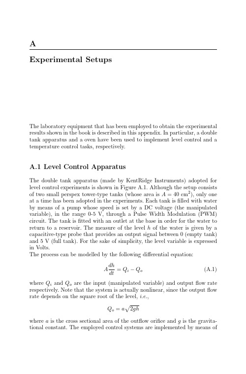
AExperimental SetupsThe laboratory equipment that has been employed to obtain the experimental results shown in the book is described in this appendix.In particular,a double tank apparatus and a oven have been used to implement level control and a temperature control tasks,respectively.A.1Level Control ApparatusThe double tank apparatus(made by KentRidge Instruments)adopted for level control experiments is shown in Figure A.1.Although the setup consists of two small perspex tower-type tanks(whose area is A=40cm2),only one at a time has been adopted in the experiments.Each tank isfilled with water by means of a pump whose speed is set by a DC voltage(the manipulated variable),in the range0-5V,through a Pulse Width Modulation(PWM) circuit.The tank isfitted with an outlet at the base in order for the water to return to a reservoir.The measure of the level h of the water is given by a capacitive-type probe that provides an output signal between0(empty tank) and5V(full tank).For the sake of simplicity,the level variable is expressed in Volts.The process can be modelled by the following differential equation:A dhdt=Q i−Q o(A.1)where Q i and Q o are the input(manipulated variable)and outputflow rate respectively.Note that the system is actually nonlinear,since the outputflow rate depends on the square root of the level,i.e.,Q o=a2ghwhere a is the cross sectional area of the outflow orifice and g is the gravita-tional constant.The employed control systems are implemented by means of296A Experimental Setupsa PC-based controller whose sampling time is5ms.It is worth noting that the two tanks(both of them have been employed in the experiments shown in the book)have a different dynamics.Further,different models arise depending on the adopted identification experiment(see Chapter 7).Fig.A.1.The double tank apparatus employed for level control experimentsA.2Temperature Control ApparatusA laboratory scale oven has been employed to implement temperature control tasks.It consists of an aluminium plate that is heated by two resistors attached to it.The plate is inserted in an insulating box(whose dimensions are33×21×16.5cm).A fan(which has not been adopted in the experiments)is present in order to provide a fast cooling of the apparatus.The temperature of the plate is measured by means of a thermocouple.The overall process is sketched in Figure A.2.The same PC-based controller(with a sampling time of5ms)of the level control experiments has been employed.The temperature process can be modelled by the following equations:C p˙τp=P−G pb(τp−τb)C b˙τb=G pb(τp−τb)+G be(τe−τb)(A.2)A Experimental Setups297 whereτp is the temperature of the plate,τb is the temperature of the box,τe is the temperature of the external environment,C p and C c are the heat capacities of the plate and of the box respectively,and G pb and G be are the thermal conductances between the plate and the box and between the box and the external environment,respectively.Finally,P is the thermal power provided by the heating elements.The control task consists of controlling the temperature of the plate by acting on the thermal power of the heating elements,namely,by manipulating the voltage across the resistors.As for the level control task,for the sake of sim-plicity the input and output are expressed in Volts(both in the range0-5V). It has to be stressed that there is not active cooling and therefore the process is asymmetric(the dynamics is different depending on the fact that the plate has to be heated or cooled).Because of this significant nonlinearity,the appa-ratus has not been adopted for those methods that relies on a linear dynamics of the process.Fig.A.2.The oven employed for level control experimentsReferencesAhmed,S., B.Huang and S.L.Shah(2006).Parameter and delay estimation of continuous-time models using a linearfilter.Journal of Process Control 16(4),323–331.Altmann,W.(2005).Practical Process Control for Engineers and Technicians.Newnes.The Netherlands.Ang,K.H.,G.Chong and Y.Li(2005).PID control systems analysis,design,and technology.IEEE Transactions on Control Systems Technology13,559–576. Araki,M.(1988).Two degree-of-freedom PID controller.Systems,Control,and In-formation42,18–25.˚A str¨o m,K.and T.H¨a gglund(2000a).Benchmark systems for PID control.In: Preprints IFAC Workshop on Digital Control PID‘00.Terrassa,E.pp.181–182.˚A str¨o m,K.J.and B.Wittenmark(1995).Adaptive Control.Addison-Wesley.˚A str¨o m,K.J.and B.Wittenmark(1997).Computer-Controlled Systems-Theory and Design.Prentice Hall.Upper Saddle River,USA.˚A str¨o m,K.J.and T.H¨a gglund(1984).Automatic tuning of simple controllers with specification on phase and amplitude margins.Automatica20(5),655–651.˚A str¨o m,K.J.and T.H¨a gglund(1995).PID Controllers:Theory,Design and Tuning.ISA Press.Research Triangle Park,USA.˚A str¨o m,K.J.and T.H¨a gglund(2000b).The future of PID control.In:Preprints IFAC Workshop on Digital Control PID‘00.Terrassa,E.pp.19–30.˚A str¨o m,K.J.and T.H¨a gglund(2004).Revisiting the Ziegler–Nichols step response method for PID control.Journal of Process Control14,635–650.˚A str¨o m,K.J.and T.H¨a gglund(2006).Advanced PID Control.ISA Press.Research Triangle Park,USA.˚A str¨o m,K.J.,H.Panagopoulos and T.H¨a gglund(1998).Design of PI controllers based on non-convex optimization.Automatica34(5),585–601.˚A str¨o m,K.J.,T.H¨a gglund,C.C.Hang and W.K.Ho(1993).Automatic tuning and adaptation for PID controllers-a survey.Control Engineering Practice 1,699–714.Atherton,D.P.(2000).Relay autotuning:a use of old ideas in a new setting.Trans-actions of the Institute of Measurement and Control22(1),103–122. Bennett,S.(2000).The past of PID controllers.In:Preprints IFAC Workshop on Digital Control PID‘00.Terrassa,E.pp.3–13.300ReferencesBequette,B.W.(2003).Process Control-Modeling,Design,and Simulation.Pren-tice A.Bj¨o rklund,S.(2003).A survey and comparison of time-delay estimation methods in linear systems.Technical Report Licentiate Thesis no.1061.Department of Electrical Engineering,Linkping University.Bohn,C.and D.P.Atherton(1995).An analysis package comparing PID anti-windup strategies.IEEE Control Systems Magazine pp.34–40.Chen,D.and D.E.Seborg(2002).PI/PID controller design based on direct synthe-sis and disturbance rejection.Industrial and Engineering Chemistry Research 41,4807–4822.Choudhury,M.A.A.S.,N.F.Thornhill and S.Shah(2005).Modelling valve stic-tion.Control Engineering Practice13(5),641–658.Choudhury,M.A.A.S.,S.L.Shah and N.F.Thornhill(2004).Detection and diag-nosis of system nonlinearities using higher order statistics.Automatica40,1719–1728.Corriou,J.-P.(2004).Process Control-Theory and A. Corripio,A.B.(2001).Tuning of Industrial Control Systems.ISA A. Daubechies,I.(1992).Ten Lectures on Wavelets.SIAM A.Devasia,S.(2002).Should model-based inverse inputs be used as feedforward under plant uncertainties?.IEEE Transactions on Automatic Control47(11),1865–1871.Devasia,S.,D.Chen and B.Paden(1996).Nonlinear inversion-based output track-ing.IEEE Transactions on Automatic Control41,930–943.Dorf,R.C.and R.H.Bishop(1995).Modern Control Systems.Addison-Wesley. Driankov,D.,H.Hellendoorn and M.Reinfrank(1993).An Introduction to Fuzzy A.Ellis,G.(2004).Control System Design A.Eriksson,P.-G.and A.J.Isaksson(1994).Some aspects of control loop performance monitoring.In:Proceedings IEEE International Conference on Control Appli-cations.Glasgow,UK.pp.1029–1034.Forsman,K.and A.Stattin(1999).A new criterion for detecting oscillations in control loops.In:Proceedings5th European Control Conference.Karlsruhe,D. Friman,M.and K.V.Waller(1997).A two-channel relay for autotuning.Industrial and Engineering Chemistry Research36,2662–2671.Gerry,J.and F.G.Shinskey(2005).PID controller specification(white paper).available on-line at /PIDspec.htm.Gomes,V.G.(1985).Controllingfired heaters.Chemical Engineering pp.63–68. H¨a gglund,T.(1995).A control-loop performance monitor.Control Engineering Practice3,1543–1551.H¨a gglund,T.(1999).Automatic detection of sluggish control loops.Control Engi-neering Practice7,1505–1511.H¨a gglund,T.(2001).The blend station-a new ratio control structure.Control Engineering Practice9,1215–1220.H¨a gglund,T.(2002).A friction compensator for pneumatic control valves.Journal of Process Control12,897–904.H¨a gglund,T.(2005).Industrial implementation of on-line performance monitoring tool.Control Engineering Practice13(11),1383–1390.H¨a gglund,T.and K.J.˚A str¨o m(2000).Supervision of adaptive control algorithms.Automatica36(2),1171–1180.References301 Hang,C.C.,A.P.Loh and V.U.Vasnani(1994).Relay feedback auto-tuning of cascade controllers.IEEE Transactions on Control Systems Technology2,42–45.Hang,C.-C.and L.Cao(1996).Improvement of transient response by means of vari-able set point weighting.IEEE Transactions on Industrial Electronics43,477–484.Hang,C.C.,K.J.˚A str¨o m and Q.G.Wang(2002).Relay feedback auto-tuning of process controllers-a tutorial review.Journal of Process Control12,143–162. Hang,C. C.,K.J.˚A str¨o m and W.K.Ho(1991).Refinements of the Ziegler–Nichols tuning formula.IEE Proceedings-Control Theory and Applications 138(2),111–118.Hansson,A.,P.Gruber and J.Todtli(1994).Fuzzy anti-reset windup for PID con-trollers.Control Engineering Practice2(3),389–396.Hanus,R.,M.Kinnaert and J.-L.Henrotte(1987).Conditioning technique,a general anti-windup and bumpless transfer method.Automatica23(6),729–739. Harriot,P.(1964).Process A.Harris,T.J.(1989).Assessment of control loop performance.The Canadian Journal of Chemical Engineering67,856–861.Harris,T.J.,C.T.Seppala and L.D.Desborough(1999).A review of performance monitoring and assessment techniques for univariate and multivariate control systems.Journal of Process Control9(1),1–17.Ho,W.K.and W.Xu(1998).PID tuning for unstable processes based on gain and phase-margin specifications.IEE Proceedings-Control Theory and Applications 145(5),392–396.Hodel, A.Scottedward and C. E.Hall(2001).Variable-structure PID control to prevent integrator windup.IEEE Transactions on Industrial Electronics 48(2),442–451.Homaifar,A.and E.McCormick(1995).Simultaneous design of membership func-tions and rule sets for fuzzy controllers using genetic algorithms.IEEE Trans-actions on Fuzzy Systems3(2),129–139.Horch,A.(1999).A simple method for detection of stiction in control valves.Control Engineering Practice7,1221–1231.Horch,A.(2000).Condition monitoring of control loops.PhD thesis.Royal Institute of Technology.Stockholm,S.Horch,A.(2001).Detection of valve stiction in integrating processes.In:Proceedings 6th European Control Conference.Porto,P.pp.1327–1332.Huang,B.(2003).A pragmatic approach towards assessment of control loop per-formance.International Journal of Adaptive Control and Signal Processing 17,589–608.Huang, B.and S.L.Shah(1999).Performance Assessment of Control Loop..Huang,C.-T.and C.-J.Chou(1994).Estimation of the underdamped second-order parameters from the system transient.Industrial and Engineering Chemistry Research33,174–176.Huang,C.-T.and M.-F.Huang(1993).Estimation of the second-order parameters from the process transient by simple calculation.Industrial and Engineering Chemistry Research32,228–230.Huang,H.-P.and J.-C.Jeng(2002).Monitoring and assessment of control perfor-mance for single loop systems.Industrial and Engineering Chemistry Research 41,1297–1309.302ReferencesHuang,H.-P.,M.-W.Lee and C.-L.Chen(2001).A system of procedures for iden-tification of simple models using transient step response.Industrial and Engi-neering Chemistry Research40,1903–1915.Hunt,L.R.and G.Meyer(1997).Stable inversion for nonlinear systems.Automatica 33(8),1549–1554.Hunt,L.R.,G.Meyer and R.Su(1996).Noncausal inverses for linear systems.IEEE Transactions on Automatic Control41,608–611.Ingimundarson,A.and T.H¨a gglund(2002).Performance comparison between PID and dead-time compensating controllers.Journal of Process Control12,887–895.Isaksson,A.J.and S.F.Graebe(1999).Analytical PID parameter expressions for higher order systems.Automatica35,1121–1130.Isaksson,A.J.and S.F.Graebe(2002).Derivativefilter is an integral part of PID design.IEE Proceedings-Control Theory and Applications149(1),41–45. Jelali,M.(2006).An overview of control performance assessment technology and industrial applications.Control Engineering Practice14,441–466.Johnson,M.A.and M.H.Moradi(eds.)(2005).PID control-New Identification and Design Methods.Springer-Verlag.London,Great Britain.Katebi,M.R.and A.W.Ordys(1996).Minimum variance control.In:The Control Handbook(W.S.Levine ed.).CRC Press.Boca Raton,FL.pp.1089–1096. Kaya,I.(2001).Improving performance using cascade control and a smith predictor.ISA Transactions40,223–234.Kaya,I.and D.P.Atherton(2005).Improved cascade control structure for con-trolling unstable and integrating processes.In:Proceedings IEEE International Conference on Decision and Control-European Control Conference.Sevilla,E.pp.7133–7138.Kaya,I.,N.Tan and D.P.Atherton(2005).Improved cascade control structure and controller design.In:Proceedings IEEE International Conference on Decision and Control-European Control Conference.Sevilla,E.pp.3055–3060.Ko,B.-S.and T.F.Edgar(2004).PID control performance assessment:the single-loop case.AIChE Journal50,1211–1218.Kothare,M.V.,P.J.Campo,M.Morari and t(1994).A unified framework for the study of anti-windup design.Automatica30(12),1869–1883.Kozub,D.J.(2002).Controller performance monitoring and diagnosis:industrial perspective.In:Preprints of the15th IFAC World Congress on Automatic Con-trol.Barcelona,E.Krishnaswami,P.R.,G.P.Rangaiah,R.K.Jha and P.D.Deshpande(1990).When to use cascade control.Industrial and Engineering Chemistry Research 29,2163–2166.Kristiansson,B.and B.Lennartson(2001).Robust and optimal tuning of PI and PID controllers.IEE Proceedings-Control Theory and Applications149(1),17–25.Kristiansson,B.and B.Lennartson(2006).Evaluation and simple tuning of PID controllers with high-frequency robustness.Journal of Process Control16,91–102.Kuehl,P.and A.Horch(2005).Detection of sluggish control loops-experiences and improvements.Control Engineering Practice13,1019–1025.Kwak,H.J.,S.W.Sung and I.-B.Lee(1997).On-line process identification and autotuning for integrating processes.Industrial and Engineering Chemistry Re-search36,5329–5338.References303 Lee,Y.,S.Oh and S.Park(2002).Enhanced control with a general cascade control structure.Industrial and Engineering Chemistry Research41,2679–2688. Lee,Y.,S.Park and M.Lee(1998a).PID controller tuning to obtain desired closed loop responses for cascade control systems.Industrial and Engineering Chem-istry Research37,1859–1865.Lee,Y.,S.Park,M.Lee and C.Brosilow(1998b).PID controller tuning for desired closed-loop responses for SI/SO systems.AIChE Journal44(1),106–115. Leva,A.(1993).PID autotuning algorithm based on relay feedback.IEE Proceedings -Control Theory and Applications140(5),328–338.Leva,A.(2005).Autotuning process controller with improved load disturbance re-jection.Journal of Process Control15,223–234.Leva,A.and A.M.Colombo(1999).Methods for optimising set-point weights in ISA-PID autotuners.IEE Proceedings-Control Theory and Applications 146(2),137–146.Leva,A.and A.M.Colombo(2001).IMC-based synthesis of the feedback block of ISA-PID regulators.In:Proceedings6th European Control Conference.Porto, P.pp.196–201.Leva,A.,C.Cox and A.Ruano(2001).Hands-on PID autotuning:a guide to bet-ter utilisation.Technical report.IF AC Technical Brief,available at .Lewin,D.R.and C.Scali(1988).Feedforward control in the presence of uncertainty.Industrial and Engineering Chemistry Research27,2323–2331.Lewis,F.L.(1996).Optimal control.In:The Control Handbook(W.S.Levine ed.).CRC Press.Boca Raton,FL.pp.759–778.Li,W.,E.Eskinat and W.L.Luyben(1991).An improved autotune identification method.Industrial and Engineering Chemistry Research30,1530–1541.Liu,T.,D.Gu and W.Zhang(2005).Decoupling two-degree-of-freedom control strategy for cascade control systems.Journal of Process Control15,159–167. Ljung,L.(1996).System identification.In:The Control Handbook(W.S.Levine ed.).CRC Press.Boca Raton,FL.pp.1033–1054.Luyben,M.L.and W.L.Luyben(1997).Essentials of Process A.Luyben,W.L.(1987).Derivation of transfer function model for highly nonlinear distillation columns.Industrial and Engineering Chemistry Research26,2490–2495.Luyben,W.L.(2001a).Effect of derivative algorithm and tuning selection on the PID control of dead-time processes.Industrial and Engineering Chemistry Re-search40,3605–3611.Luyben,W.L.(2001b).Getting more information from relay-feedback tests.Indus-trial and Engineering Chemistry Research40,4391–4402.Macvicar-Whelan,P.J.(1976).Fuzzy sets for man-machine interaction.Interna-tional Journal of Man-Machine Studies8,687–697.Majhi,S.and D.P.Atherton(2000).Online tuning of controllers for an un-stable FOPDT process.IEE Proceedings-Control Theory and Applications 147(4),421–427.Marlin,T.E.(2000).Process Control:Designing Processes and Control Systems for Dynamic A.Miao,T.and D.E.Seborg(1999).Automatic detection of excessively oscillatory feedback loops.In:Proceedings IEEE International Conference on Control Ap-plications.Kohala Coast,HW.pp.359–364.304ReferencesMitchell,M.(1998).An Introduction to Genetic Algorithms.MIT A. Morari,M.and E.Zafiriou(1989).Robust Process Control.Prentice Hall.Englewood Cliffs,NJ.O’Dwyer,A.(2006).Handbook of PI and PID Tuning Rules.Imperial College Press. Ogunnaike,B.A.and W.H.Ray(1994).Process Dynamics,Modeling,and Control.Oxford University A.Palmor,Z.J.(1996).Time-delay compensation-Smith predictor and its modifica-tions.In:The control handbook(W.S.Levine ed.),CRC Press.pp.224–237. Panagopoulos,H.,K.J.˚A str¨o m and T.H¨a gglund(2002).Design of PID controllers based on constrained optimisation.IEE Proceedings-Control Theory and Ap-plications149(1),32–40.Panda,R.C.(2006).Estimation of parameters of under-damped second order plus dead time processes using relay puters and Chemical Engineering 30(5),832–837.Panda,R.C.and C.-C.Yu(2003).Analytical expressions for relay feed back re-sponses.Journal of Process Control13,489–501.Panda,R.C.and C.-C.Yu(2005).Shape factor of relay response curves and its use in autotuning.Journal of Process Control15,893–906.Panda,R.C.,C.-C.Yu and H.-P.Huang(2004).PID tuning rules for SOPDT systems:review and some new results.ISA Transactions43,283–295.Park,H.I.,S.W.Sung,I.-B.Lee and J.Lee(1997).On-line process identification us-ing Laguerre series for automatic tuning of the proportional–integral–derivative controller.Industrial and Engineering Chemistry Research36,101–111. Patwardhan,R.S.and S.L.Shah(2002).Issues in performance diagnostics of model-based controllers.Journal of Process Control12,413–417.Paulonis,M.A.and J.W.Cox(2003).A practical approach for large-scale controller performance assessment,diagnosis,and improvement.Journal of Process Con-trol13,155–168.Peng,Y.,D.Vrancic and R.Hanus(1996).Anti-windup,bumpless,and conditioned transfer techniques for PID controllers.IEEE Control Systems Magazine pp.48–57.Perez,H.and S.Devasia(2003).Optimal output transitions for linear systems.Automatica39,181–192.Petersson,M.,K.-E.˚A rz`e n and T.H¨a gglund(2001).Assessing measurements for feedforward control.In:Proceedings of the6th European Control Conference.Porto,P.Petersson,M.,K.-E.Arzen and T.H¨a gglund(2003).A comparison of two feedfor-ward control structure assessment methods.International Journal of Adaptive Control and Signal Processing17,609–624.Pfeiffer,B.-M.(1999).Towards Plug&Control:selftuning temperature controller for plc.In:Proceedings5th European Control Conference.Karlsruhe,D.Pfeiffer, B.-M.(2000).Towards‘plug and control’:self-tuning temperature con-troller for PLC.International Journal of Adaptive Control and Signal Processing 14,519–532.Piazzi,A.and A.Visioli(2000).Minimum-time system-inversion-based motion plan-ning for residual vibration reduction.IEEE/ASME Transactions on Mechatron-ics5(1),12–22.Piazzi,A.and A.Visioli(2001a).Optimal inversion-based control for the set-point regulation of nonminimum-phase uncertain scalar systems.IEEE Transactions on Automatic Control46,1654–1659.References305 Piazzi,A.and A.Visioli(2001b).Optimal noncausal set-point regulation of scalar systems.Automatica37(1),121–127.Piazzi,A.and A.Visioli(2001c).Robust set-point constrained regulation via dy-namic inversion.International Journal of Robust and Nonlinear Control11,1–22.Piazzi, A.and A.Visioli(2005).Using stable input-output inversion for minimum-time feedforward constrained regulation of scalar systems.Automat-ica41(2),305–313.Piazzi,A.and A.Visioli(2006).A noncausal approach for PID control.Journal of Process Control16,831–843.Press,W.H.,S.A.Teukolsky,W.T.Vetterling and B.P.Flannery(1995).Nu-merical Recipes:The Art of Scientific Computing.Cambridge University Press.Cambridge,UK.Qin,S.J.(1998).Control performance monitoring-a review and -puters and Chemical Engineering23,173–186.Ramakrishnan,V.and M.Chidambaram(2003).Estimation of a SOPDT transfer function model using a single asymmetrical relay feedback puters and Chemical Engineering27,1779–1784.Rangaiah,G.P.and P.R.Krishnaswamy(1994).Estimating second-order plus dead time model parameters.Industrial and Engineering Chemistry Research 33,1867–1871.Rangaiah,G.P.and P.R.Krishnaswamy(1996).Estimating second-order dead time parameters from underdamped process transient.Chemical Engineering Science 51(7),1149–1155.Rivera,D.E.,S.Skogestad and M.Morari(1986).Internal model control.4.PID controller design.Industrial and Engineering Chemistry Process Design and De-velopment25(1),252–265.Rossi,M.and C.Scali(2005).A comparison of techniques for automatic detection of stiction:simulation and application to industrial data.Journal of Process Control15(5),505–514.Salsbury,T.I.(2005).A practical method for assessing the performance of control loops subject to random load changes.Journal of Process Control15(4),393–405.Scali,C.and D.Semino(1991).Performance of optimal and standard controllers for disturbance rejection in industrial processes.In:Proceedings IEEE International Conference on Industrial Electronics,Control,and Instrumentation.Kobe,J.pp.2033–2038.Scali,C.,G.Marchetti and D.Semino(1999).Relay with additional delay for iden-tification and autotuning of completely unknown processes.Industrial and En-gineering Chemistry Research38,1987–1997.Seborg,D.E.,T.E.Edgar and D.A.Mellichamp(2004).Process Dynamics and Control-2nd A.Shen,S.-H.,J.-S.Wu and C.-C.Yu(1996).Use of a biased relay feedback for system identification.American Institute of Chemical Engineering Journal42,1174–1180.Shinskey,F.G.(1994).Feedback Controllers for the Process Industries.McGraw-Hill.New York.Shinskey,F.G.(1996).Process Control Systems-Application,Design,and Tuning.McGraw-Hill.New York,USA.306ReferencesShinskey,F.G.(2000).PID-deadtime control of distributed processes.In:Preprints IFAC Workshop on Digital Control PID’00.pp.14–18.Silva,G.J.,A.Datta and S.P.Bhattacharyya(2002).Robust control design using the PID controller.In:Proceedings IEEE International Conference on Decision and s Vegas,USA.pp.1313–1318.Singhal,A.and T.I.Salsbury(2005).A simple method for detecting valve stiction in oscillating control loops.Journal of Process Control15(4),371–382. Skogestad,S.(2003).Simple analytic rules for model reduction and PID controller tuning.Journal of Process Control13,291–309.Srinivasan,K.and M.Chidambaram(2003).Modified relay feedback method for improved system identifiputers and Chemical Engineering27,727–732.Sundaresan,K.R.and P.R.Krishnaswamy(1978).Estimation of time delay,time constant parameters in time,frequency and Laplace domains.Canadian Journal of Chemical Engineering56,257–262.Sundaresan,K.R.,C.Chandra Prasad and P.R.Krishnaswamy(1978).Evaluat-ing parameters from process transients.Industrial and Engineering Chemistry Process Design and Development17,237–241.Sung,S.W.,I.-B.Lee and B.-K.Lee(1998).On-line process identification and automatic tuning method for PID controllers.Chemical Engineering Science 53,1847–1859.Swanda,A.P.and D.E.Seborg(1999).Controller performance assessment based on set-point response data.In:Proceedings American Control Conference.San Diego,CA.pp.3863–3867.Taha,O.,G.A.Dumont and M.S.Davies(1996).Detection and diagnosis of os-cillations in control loops.In:Proceedings IEEE International Conference on Decision and Control.Kobe,J.pp.2432–2437.Tan,K.K.,Q.-G.Wang,C.C.Hang and T.H¨a gglund(1999).Advances in PID control.Springer-Verlag.London,Great Britain.Tan,K.K.,T.H.Lee and R.Ferdous(2000).Simultaneous online automatic tuning of cascade control for open loop stable processes.ISA Transactions39,233–242. Thornhill,N.F.and T.H¨a gglund(1997).Detection and diagnosis of oscillation in control loop.Control Engineering Practice5(10),1343–1354.Thornhill,N.F.,B.Huang and S.L.Shah(2003).Controller performance assessment in set point tracking and regulatory control.International Journal of Adaptive Control and Signal Processing17,709–727.Thyagarajan,T.and C.-C.Yu(2003).Improved autotuning using the shape factor from relay feedback.Industrial and Engineering Chemistry Research42,4425–4440.Thyagarajan,T.,C.-C.Yu and H.-P.Huang(2003).Assessment of controller perfor-mance:a relay feedback approach.Chemical Engineering Science58,497–512. Tzafestas,S.G.(1994).Fuzzy systems and fuzzy expert control:an overview.The Knowledge Engineering Review9(3),229–268.Visioli,A.(1999).Fuzzy logic based set-point weight tuning of PID controllers.IEEE Transactions on Systems,Man,and Cybernetics-Part A29,587–592. Visioli,A.(2000).Adaptive tuning of fuzzy set-point weighting for PID controllers.In:Preprints IFAC Workshop on Digital Control PID‘00.Terrassa,E.pp.513–518.Visioli,A.(2001a).Optimal tuning of PID controllers for integral and unstable processes.IEE Proceedings-Control Theory and Applications148(2),180–184.References307 Visioli,A.(2001b).Tuning of PID controllers with fuzzy logic.IEE Proceedings-Control Theory and Applications148(1),1–8.Visioli,A.(2003a).Modified anti-windup scheme for PID controllers.IEE Proceed-ings-Control Theory and Applications150(1),49–54.Visioli,A.(2003b).Time-optimal plug&control for integrating and FOPDT pro-cesses.Journal of Process Control13,195–202.Visioli,A.(2004).A new design for a PID plus feedforward controller.Journal of Process Control14,455–461.Visioli,A.(2005a).Design and tuning of a ratio controller.Control Engineering Practice13,485–497.Visioli,A.(2005b).Experimental evaluation of a Plug&Control strategy for level control.In:Preprints16th IFAC World Congress on Automatic Control.Prague, CZ.Visioli,A.(2005c).Model-based PID tuning for high-order processes:when to ap-proximate.In:Proceedings IEEE International Conference on Decision and Control-European Control Conference.Sevilla,E.pp.7127–7132.Visioli,A.(2005d).A new ratio control architecture.Industrial and Engineering Chemistry Research44,4617–4624.Visioli,A.(2006).Method for proportional-integral controller tuning assessment.Industrial and Engineering Chemistry Research45,2741–2747.Visioli,A.and A.Piazzi(2003).Improving set-point following performance of in-dustrial controllers with a fast dynamic inversion algorithm.Industrial and En-gineering Chemistry Research42,1357–1362.Visioli,A.and A.Piazzi(2005).On the use of dynamic inversion for the improvement of PID control.In:Preprints16th IFAC World Congress on Automatic Control.Prague,CZ.Visioli,A.and A.Piazzi(2006).An automatic tuning method for cascade control systems.In:Proceedings IEEE International Conference on Control Applica-tions.Munich,D.Visioli,A.and M.Veronesi(1999).Nuove funzionalita’per controllori PID(in ital-ian).Automazione e Strumentazione(October),149–155.Vivek,S.and M.Chidambaram(2005a).Identification using single symmetrical relay feedback puters and Chemical Engineering29,1625–1630. Vivek,S.and M.Chidambaram(2005b).An improved relay autotuning of PID controllers for unstable FOPDT puters and Chemical Engineering 29,2060–2068.Vrancic,D.(1997).Design of anti-windup and bumpless transfer protection.PhD thesis.University of Ljubljana.Ljubljana,SLO.Walgama,K.S.and J.Sternby(1990).Inherent observer property in a class of anti-windup compensators.International Journal of Control52(3),705–724. Walgama,K.S.,S.Ronnback and J.Sternby(1991).Generalisation of conditioning technique for anti-windup compensator.IEE Proceedings-Control Theory and Applications139(2),109–118.Wallen,A.(2000).Tools for autonomous process control.PhD thesis.Lund Institute of Technology.Lund,S.Wallen,A.and K.J.˚A str¨o m(2002).Pulse-step control.In:Preprints of the15th IFAC World Congress on Automatic Control.Barcelona,E.Wang,L.and W.R.Cluett(1994).Optimal choice of time-scaling factor for linear system approximations using laguerre models.IEEE Transactions on Automatic Control39(7),1463–1467.。

In the realm of future technology,our imaginations can run wild.Heres a detailed English composition that envisions the technological advancements of the future.Title:A Glimpse into the Future of TechnologyAs we stand on the precipice of the next era of technological innovation,it is both thrilling and daunting to consider the potential changes that lie ahead.The future of technology promises to be a tapestry woven with threads of artificial intelligence, quantum computing,biotechnology,and sustainable energy solutions.Artificial Intelligence AIThe integration of AI into daily life will be seamless and ubiquitous.Personal AI assistants will not only manage our schedules and provide information but will also understand our emotions and predict our needs.In the workplace,AI will collaborate with humans to enhance productivity,offering insights and solutions that we might not have considered.Autonomous vehicles will revolutionize transportation,reducing accidents and traffic congestion while optimizing routes for efficiency.Quantum ComputingQuantum computers will unlock new frontiers in data processing and problemsolving. With their ability to perform complex calculations at unprecedented speeds,they will transform fields such as cryptography,drug discovery,and materials science.Quantum encryption will ensure unprecedented security in digital communications,while quantum simulations will enable the design of new materials with tailored properties. BiotechnologyAdvancements in biotechnology will lead to breakthroughs in personalized medicine. Genetic editing technologies like CRISPR will allow us to correct genetic disorders and potentially enhance human capabilities.Synthetic biology will give rise to new forms of life,designed to perform specific functions,such as cleaning up pollution or producing renewable energy.Sustainable EnergyThe quest for sustainable energy will yield innovative solutions to combat climate change. Solar and wind energy will become more efficient and affordable,with advancements in energy storage allowing for a more stable and reliable power grid.Fusion power,once adream of science fiction,may become a reality,providing a nearly limitless and clean source of energy.Virtual and Augmented RealityThe boundaries between the digital and physical worlds will blur as virtual reality VR and augmented reality AR become more sophisticated.VR will offer immersive experiences for entertainment,education,and therapy,while AR will overlay digital information onto the physical world,enhancing our perception and interaction with the environment.Space ExplorationThe future will see a new age of space exploration,with private companies and international collaborations pushing the limits of what we know.Mars may become the first offworld colony,with sustainable habitats and infrastructure built to support human life.Space tourism will become a reality,offering breathtaking views of Earth from the cosmos.CybersecurityAs our reliance on technology grows,so does the importance of cybersecurity.Advanced encryption methods and AIdriven threat detection systems will protect our digital infrastructure from cyber attacks.Quantumresistant algorithms will safeguard our data against the power of quantum computers.Ethical ConsiderationsWith great power comes great responsibility.The future of technology will demand a robust ethical framework to guide its development and use.Issues such as privacy,data ownership,and the digital divide will require thoughtful solutions to ensure that technological advancements benefit all of humanity.In conclusion,the future of technology is a canvas waiting for the brushstrokes of innovation.It holds the promise of a world that is more connected,efficient,and sustainable.However,it also presents challenges that we must navigate with wisdom and foresight.As we step into this future,let us do so with a commitment to using technology for the betterment of all.。

第42卷第11期2020年11月舰船科学技术SHIP SCIENCE AND TECHNOLOGYVol.42,No.11Nov., 2020潜艇隐身技术分析闫大海，张啥，苗金林，杨晓刚(中国舰船研究院，北京100101)摘要：本文分析研究包括声波、电磁波、尾流等在内探测潜艇的主要技术手段，以及针对这些手段，潜艇所采取的包括声隐身、雷达波隐身、尾迹隐身等在内的主要隐身措施。

系统提出探测技术发展趋势。

潜艇隐身技术难度大、涉及专业广，集成度高，需要以需求为牵引，密切跟踪探测技术发展趋势，坚持从设计源头贯彻隐身设计思想，同时不断提高潜艇对不同侦察制导和攻击手段的软硬杀伤能力，探索新技术、新手段，保证我潜艇在现代海战中处于优势地位。

关键词：探测；潜艇；隐身中图分类号：U674文献标识码：A文章编号：1672-7649(2020)11-0128-06doi：10.3404/j.issn,1672-7649.2020.11.026Research on submarine stealth technologyYAN Da-hai,ZHANG Han,MIAO Jin-lin,YANG Xiao-gang(China Ship Research and Development Academy,Beijing100101,China)Abstract:This paper analyzes the main technical ways of detecting submarine,including acoustic wave,electromag­netic wave,wake flow and so on,as well as the main stealth measxires taken for these ways,including acoustic stealth,radar wave stealth,wake stealth and so on.The development trend of detection technology is put forward systematically.The stealth technology of submarines is very difficult,involving a wide range of specialties and high integration.It needs to closely follow the development trend of detection technology,adhere to the stealth design idea from the design source,and constantly improve the soft and hard lethality of submarines to different reconnaissance guidance and attack means,explore new technologies and new means,so as to ensure that our submarines are in an advantageous position in modem naval war­fare.Key words:detection;submarine;stealtho引言潜艇的优势在于隐蔽性。

.40中国医疗器械信息 | China Medical Device Information标准检测Standard and T esting鉴于新版国际标准ISO 8637:2010《心血管植入物和体外系统 血液透析器、血液透析滤过器、血液滤过器和血液浓缩器》已发布，且该标准尚未转化成我国新版行业标准，与ISO8637:2004对比，超滤系数已经重新定义且修改了检测方法，本文将对该项目具体检测进行诠释，希望能为国内血液透析器生产厂家对超滤系数的确定提供参考。

如何检测血液透析器超滤系数蓝建华 国家食品药品监督管理局广州医疗器械质量监督检验中心 （广州 510080）内容提要： 目的：探讨新版国际标准ISO 8637:2010中超滤系数的分析检测方案。

方法：计算滤过液流率和跨膜压之间的回归线斜率作为超滤系数。

结论：通过该方案可以确定血液透析器产品的超滤系数。

How to Test Ultrafiltration Coefficient of HaemodialyserLAN Jian-hua Guangzhou Quality Supervision and Iuspection Center for Medical Devices (Guangzhou 510080)Abstract:Objective : To discuss the detection program of ultrafiltration coefficient from ISO 8637:2010. Method : Calculate the ultrafiltrationcoefficient as the slope of the regression line between filtration flow rate and transmembrane pressure. Result : Ultrafiltration coefficient of haemodialyser can be established by the detection program.Key words:ultrafiltration coefficient, transmembrane pressure, filtration flow rate1.实验材料、试剂及设备1.1实验材料空心纤维透析器：低通量透析器和高通量透析器各一支。

不连续介质反演的原对偶牛顿法和全变差正则化冯立新;李媛;张磊【摘要】研究利用散射场测量数据反演非均匀介质的逆散射问题,特别是平面波在非均匀介质中传播时所产生逆散射问题的数值计算.为克服非均匀介质不连续变化和反演具有不适定性的困难,提出基于全变差正则化的原对偶牛顿方法,避免了一般正则化方法对不连续介质交界处反演的过光滑性作用.数值试验显示,本算法可以在观测数据带有一定噪声的境况下有效地重构不连续介质系数.%An inverse scattering problem of inhomogeneous mediums from the measurements of the scattered field is considered.In particular,it focuses on the numerical computation of the inverse scattering generated by the interaction of a plane wave and an inhomogeneous medium.To solve the ill-posedness as well as the difficulties caused by inhomogeneous media,a primal-dual Newton method based on the total variation regularization is constructed.The overly smooth effect of the usual regularization method for the inversion is overcome.Numerical experiments show that this method can recover discontinuous coefficients under moderate amount of noise in the observation data.【期刊名称】《黑龙江大学自然科学学报》【年(卷),期】2018(035)001【总页数】9页(P1-9)【关键词】全变差正则化;原对偶牛顿法;逆介质散射【作者】冯立新;李媛;张磊【作者单位】黑龙江大学数学科学学院,哈尔滨150080;黑龙江大学数学科学学院,哈尔滨150080;黑龙江大学数学科学学院,哈尔滨150080【正文语种】中文【中图分类】O1750 IntroductionIn this paper, we focus on the inverse medium scattering problem of determining electromagnetic properties of unknown inhomogeneous objects embedded in a homogeneous background from noisy measurements of the scattered field corresponding to one incident wave impinged on the objects. We describe the scattering model mathematically as follows:Δu(x)+k2η(x)u(x)=0, x∈R2,(1)where u is the total field, k is the wavenumber, η(x)>0 for all x, andm(x)=1-η(x) is the scatterer with a compact support. We assume that B containing the compact support of the scatterer m(x) be a bounded domain in R2. Let ui which is assumed to satisfyΔui+k2ui=0, x∈R2,(2)denote the incident on the inhomogeneity. Assume that the incident fieldui is a plane wave, i.e., ui(x)=exp(ikd·x), where d∈R2 is the propagation direction (a unit vector). The total field u consists of the incident field ui and the scattered field us, that is,u=ui+us.It follows immediately from Eqs. (1) and (2) that the scattered field satisfies Δus+k2us=k2m(x)ui, x∈R2,(3)and the scattered field is required to satisfy the following Sommerfeld radiation condition(4)uniformly in all directions x/|x|.The inverse medium scattering problems arise naturally in many applications such as geophysical exploration, medical imaging, and radar detection [1-5]. For the practical significance of the inverse problem, some inverse scattering methods have been developed in the literature, which may be divided into two categories: the direct methods and the indirect methods. The direct methods aims at detecting the scatterer support and shape, and includes linear sampling method (LSM)[6-8], factorization method (paper [9], Chapter 5, paper [10]), and multiple signal classification (MUSIC)[11-13]. In contrast, the indirect methods provides a distributed estimate of the refractive index by applying regularization techniques. We just mention recursive linearization [14-18] , Gauss-Newton method [19-21], and level set method [22] for an incomplete list. Generally, theestimates by an indirect method can provide more details of inclusions, but at the expense of increased computational efforts. There has been considerable interest in considering efficient and stable inversion techniques. However, due to the strong nonlinearity of the map from the refractive index to the scattered field, severe ill-posedness of the inverse problem and the limited availability of the scattered data, it is still a very challenging problem.In this work, we assume that the scattered data with fixed wavenumber are known in the domain B, i.e., the scattered field is measured forxj∈B,j=1,…,J for a given incident field. We develop an iterated method for accurately detecting the scatterer support. In the case, from the Lippmann-Schwinger integral equation, the inverse problem can be seen as the operator equation of the first kind with unknown m(x). An efficient numerical method is presented for solving the inverse medium scattering problem which is to reconstruct the inhomogeneous medium from inner measurements of the scattered field. We construct the total variation (TV) regularization approximation of the integral equation. The main reason of choosing TV regularization is that TV can penalize highly oscillatory solutions while allowing jumps in the regularized solution. Consequently, a primal-dual Newton method is used to minimize the TV functional [23-25]. This is an iterated method, which need solve direct scattering problem for each step of the process. The scattering data is generated by numerical solution of the direct scattering problem, which is implemented by using the efficient fast algorithm [26]. In this work, we develop a TVregularization and primal-dual method for solving the inverse medium problem with discontinuous coefficients. The remainder of the paper is organized as follows. Section 1 gives the integral formulation of inverse medium problem (1)～(4) and describes the TV regularization approximation. In Section 2, we employ a primal-dual Newton method for solving the corresponding inverse problem. Section 3 presents the numerical results for the inverse medium problem. Finally, we give the relevant conclusions in Section 4.1 Formulation of the integral equation and TV approximationThe integral formulation of problem (1)～(4) is the main ingredient in the proposed method. Let be the Hankel function of first kind and order 0, see paper [1] for details. We have the following Lippmann-Schwinger integral equation for u:(5)K(x,y)m(y)dy.So, we have following operator equation(Km)(x)=g.Define the Tikhonov-TV functional(6)where TV(m) is the TV of a function m defined on the B. If m is smooth, one can obtain the representation|m|dx.However, the representation is not suitable for the implementation of the numerical procedure, due to the nondifferentiability of the Euclidean norm at the origin. To overcome this difficulty, one can take an approximation to the Euclidean norm |x| like where β is a small positive parameter. This yields the following approximation to TV(m):Instead of the Tikhonov-TV functional (6), we will consider minimization of the functional(7)Suppose m=mi,j is defined on an equispaced grid in two space dimensions, {(x1i,x2j)|x1i=iΔx1,x2j=jΔx2,i=0,…,n1,j=0,…,n2}. We defi ne the discrete penalty functional Jβ(m):R(n1+1)×(n2+1)→R by(8)where To simplify notation, we drop a factor of Δx1Δx2 from the right-hand side of (8). This factor can be absorbed in the regularization α in (7). In the following section, we consider minimization of the discretized functional:(9)where the matrix K is a discretization of the operator K, the vector g and J denote discrete data, and discretization of TV approximation Jβ,respectively.2 A primal-dual Newton methodTo minimize the functional (9), the primal-dual Newton method is employed. Consider the convex functional defined on C=R2. One can show that the conjugate set C* is the unit ball in R2 and corresponding conjugate functional to φβ is(10)We can obtain the dual representation by (10):(11)The following theorem relates the gradient of a convex functional φβ to the gradient of its conjugate see paper [25], p.138 for a proof.Theorem 1 Suppose that φβ is differentiable in a neighborhood ofx0∈C⊂Rd, and the mapping F=gradφβ:Rd→R d is invertible in that neighborhood. Then is Frechét differentiable in a neighborhood ofy0=φβ(x0) withEmploying the dual representation (11), we obtain(12)We stack the array components mi,j,ui,j and vi,j into column vector m,u, and v, let Dx1 and Dx2 be matrix representation for the grid operators and and let <·,·> denote the Euclidean inner product. Then (12) can be rewritten asMinimization of the least squares functional (10) is equivalent to computing the saddle point(u*,v*,m*(13)where We refer to m as the primal variable, and to u and v as the dual variables.Since (13) is unconstrained with respect to m, a first order necessary condition for a saddle point is(14)An additional necessary condition is that the duality gap in (11) must vanish, i.e., for each grid index i, j,(15)Finally, the dual variables must lie in the conjugate set, i.e.,(ui,j,vi,j)∈C*.(16)Suppose (15) holds for a point (ui,j,vi,j) in the interior of C*. ThenUsing Theorem 1, above equations is equivalent toDx1m=B(m)u, Dx2m=B(m)v,(17)where B(m)=diag(1/ψ′(m)).We can reformulate the first order necessary conditions (14) and (17) as a nonlinear system:(18)The derivative of G can be expressed asHere B′(m)u has matrix representationB′(m)u-Dx1=-E11Dx1-E12Dx2(19)withwhere the products and quotients are computed pointwise. Similarly,B′(m)v-Dx2=-E21Dx1-E22Dx2(20)withNewton’s method for the system (18) requires solutions of systems of the formG′(u,v,m)(Δu,Δv,Δm)=-G(u,v,m).Substituting (19)～(20) and app lying block row reduction to convert G′ to block upper triangular form, consequently we obtainwhereandWe employ backtracking to the boundary to maintain the constraint (16). In other words, we computeall i,j}.We then updateAlgorithm Primal-dual Newton’s method for TV functional.ν:=0;m0:=initial guess for primal variable;u0,v0:=initial guess for dual variables;begin primal-dual Newton iterations;Δm:=[KTK+αLν]-1rν;mν+1:=mν+Δm;τν:=max{0≤τ≤1|(uν+τΔu,vν+τΔv)∈C*};uν+1:=uν+τνΔu;vν+1:=vν+τνΔv;ν:=ν+1;end primal-dual Newton iteration.3 Numerical experimentsSome numerical examples are presented to illustrate the performance of the proposed method. Here, the scattering data are generated by numerical solution of the direct scattering problem, which is implemented by using the efficient fast algorithm (see Appendix).In experiments we consider the following inhomogeneities,★ the scattered fields are measured on the domain B=[-2,2]×[-2,2];★ the incident direction d=(cos(π/3),sin(π/3)), and wa ve number k=1;★ {Qi,j⊂R2,i=1,2,…,n1,j=1,2,…,n2} is a partition of B;★ the parameters n1=20(40),n2=20(40), α=0.001, β=0.05.Fig.1 True scatterer (n1)Fig.2 Reconstruction n1 using primal-dual Newton’s methodFig.3 True scatterer (n2)Fig.4 Reconstruction n2 using primal-dual Newton’s methodTo test the stability, some relative random noise is added to the data, i.e., the measurement data takes the formu|B:=(1+δrand)u|B,where ‘rand’ gives the Gaussian white noise and δ is a noise level parameter taken to be 5% in our numerical experiments.We have set the parameter α in the TV formulation. Then, we use the above primal-dual Newton’s algorithm to solve the inverse problem. The stopping criterion for the iteration is a relative decrease of the nonlinear residual by a factor of 10-4 or through 50 times iterations. Here, the initial guess for m can be chosen for different constant. The reconstruction got faster when the the initial guess for m is better. Fig.2 and Fig.4 present reconstruction results of the refractive index from the measurement data. We can see that the method has the ability to resolve the inverse medium problem with discontinuous coefficients efficiently.4 ConclusionsWe have proposed and discussed a reconstruction technique of the inverse medium problem with discontinuous coefficients based on the measurements of the scattering field. Our aim to overcome the difficulties caused by the the ill-posedness as well as the difficulties caused by inhomogeneous media has been realized. To make the discontinuous coefficients of the medium can be reliably reconstructed, we convert the problem to an equivalent optimization problem, and then introduce the regularization term. At the same time, we use primal dual Newton method to solve the above problem. Finally, an inversion algorithm, based on TV regularization, for the inverse medium problem from the measurement data of the scattered field is shown. Numerical experiments show that the method is effective.AppendixHere, we give a fast algorithm to solve forward scattering problem (1)～(4).The method was proposed by Nadaniela Egidi etc, see paper [26] for details. The problem (1)～(4) can be reformulated as a Fredholm integral equation (5) of the second kind:Let {Ql,j⊂R2,l=1,2,…,n1,j=1,2,…,n2} be a p artition of B, the integral equation (5) is discretized as follows:(21)where ξl,j∈R2 is the center of ml,j=m(ξl,j), and ul,j is an approximation of u(ξl,j). Linear system (21) can be rewritten as following formAu=b,where b∈Cn1n2 contains u∈Cn1n2 contains ul, j, and the entry of matrix A, at row corresponding to indices l,j, and at column corresponding to i1, j1, containswhere δ is the Kronecker function.In following we give an approximation of the coefficient matrix A by using the properties of Hankel functions We havewhere J0 is the Bessel function of order 0, and Y0 is the Newmann function of order 0. From the power series expansions of these functions we have tlρ2l, ρ>0,where γ≈0.577 215 7 is the Euler constant, andhere B>0 is a suitable constant that depends on the size of D, and L is a truncation parameter.Substituting above express into (21), we obtain the following linear system:(22)where is the approximation of ul,j .We restrict our attention to coordinate partitions of B, whereQl,j,l=1,…,n1,j=1,…,n2 are given by rectangles having edges parallel to the coordinate axes. Moreover, we use the following notations :Ql,j=[al,bl]×[aj,bj],ξl,j=(ξ1l,ξ2j)∈R2,l=1,…,n1,j=1,…,n2. So, calculating the integral in (22), and rearranging the resulting terms, we obtain-×(-ξ1l)2q+1-l(-ξ2j)2p-2q+1-s)-,l=1,…,n1,j=1,…,n2.(23)Linear system (23) can be solved efficiently due to the special structure of its coefficient matrix, which is given by the identity matrix plus 2(L+1)2 rank-one matrices. We conclude that (23) can be rewritten as follows :(I+UVT)u=b,where U,V are following complex matrices having n1n2 rows and 2(L+1)2 columns.here×(-ξ1,i1)2q+1-l(-ξ2,i2)2p-2q+1-s,i1=1,2,...,n1,i2=1,2,...,n2，M=2L+1,N(l)=2L-2⎣l/2」+1.References[1] COLTON D, KRESS R. Inverse acoustic and electromagnetic scattering theory [M]. Berlin: Springer-Verlag, 1998.[2] CUI T J, CHEW W C, AYDINER A. Inverse scattering of two-dimensional dielectric objects buried in a lossy earth using the distorted Born iterative method [J]. IEEE Transactions on Geoscience and Remote Sensing, 2001, 39(2): 339-346.[3] BAO G, LI P. Numerical solution of an inverse medium scattering problem for Maxwell’s equations at fixed frequency [J]. Journal of Computational Physics, 2009, 228(12): 4638-4648.[4] BAO G, CHOW S N, LI P, et al. Numerical solution of an inverse medium scattering problem with a stochastic source [J]. Inverse Problems, 2010, 26 (7): 74014.[5] BAO G, LIN J, MEFIRE S M. Numerical reconstruction of electromagnetic inclusions in three dimensions [J]. SIAM Journal on Imaging Sciences, 2014, 7(1): 558-577.[6] CAKONI F, COLTON D, MONK P. The linear sampling method in inverse electromagnetic scattering [M]. Philadelphia: SIAM, 2010.[7] ITO K, JIN B, ZOU J. A direct sampling method to an inverse medium scattering problem [J]. Inverse Problems, 2012, 28(2): 25003.[8] ITO K, JIN B, ZOU J. A direct sampling method for inverse electromagnetic medium scattering [J]. Inverse Problems, 2013, 29(9): 95018.[9] KIRSCH A, GRINBERG N. The factorization method for inverse problems [M]. Oxford: Oxford University Press, 2008.[10] KIRSCH A. The MUSIC-algorithm and the factorization method in inverse scattering theory for inhomogeneous media [J]. Inverse Problems, 2002, 18(4): 1025-1040.[11] AMMARI H, IAKOVLEVA E, LESSELIER D, et al. MUSIC-type electromagnetic imaging of a collection of small three-dimensional inclusions [J]. SIAM Journal on Scientific Computing, 2007, 29(2): 674-709.[12] CHEN X D, ZHONG Y. MUSIC electromagnetic imaging with enhanced resolution for small inclusions [J]. Inverse Problems, 2009, 25(1): 15008. [13] BAO G, HOU S, LI P. Inverse scattering by a continuation method with initial guesses from a direct imaging algorithm [J]. Journal of Computational Physics, 2007, 227(1): 755-762.[14] BAO G, LI P. Inverse medium scattering for the Helmholtz equation at fixed frequency [J]. Inverse Problems, 2005, 21(5): 1621-1641.[15] BAO G, LI P. Numerical solution of inverse scattering for near-field optics [J]. Optics Letters, 2007, 32(11): 1465-1467.[16] BAO G, LIU J. Numerical solution of inverse scattering problems with multi-experimental limited aperture data [J]. SIAM Journal on ScientificComputing, 2003, 25(3): 1102-1117.[17] BAO G, TRIKI F. Error estimates for the recursive linearization of inverse medium problems [J]. Journal of Computational Mathematics, 2010, 28(6): 725-744.[18] BAO G, LI P, LIN J, et al. Inverse scattering problems with multi-frequencies [J]. Inverse Problems, 2015, 31 (9): 93001.[19] ZAEYTIJD D J, FRANCHOIS A, EYRAUD C, et al. Full-wave three-dimensional microwave imaging with a regularized Gauss-Newton method-theory and experiment [J]. IEEE Transactions on Antennas and Propagation, 2007, 55(11): 3279-3292.[20] HOHAGE T, LANGER S. Acceleration techniques for regularized Newton methods applied to electromagnetic inverse medium scattering problems [J]. Inverse Problems, 2010, 26(7): 74011.[21] KRESS R, RUNDELL W. Inverse scattering for shape and impedance [J]. Inverse Problems, 2001, 17(4): 1075-1085.[22] DORN O, LESSELIER D. Level set methods for inverse scattering: some recent developments [J]. Inverse Problems, 2009, 25(12): 125001.[23] BAO G, HUANG K, LI P, et al. A direct imaging method for inverse scattering using the generalized Foldy-Lax formulation [J]. Contemporary Mathematics, 2014, 615: 49-70.[24] CHAN T F, GOLUB G H, MULET P. A nonlinear primal-dual method for total varlation-based 冯立新image restoration [J]. SIAM Journal on Scientific Computing, 1999, 20(6): 1964-1977.[25] VOGEL C R. Computational methods for inverse problems [J].Philadelphia: SIAM, 2002.[26] EGIDI N, GOBBI R, MAPONI P. The efficient solution of electromagnetic scattering for inhomogeneous media [J]. Journal of Computational and Applied Mathematics, 2007, 210(1-2): 175-182.。