HYPERMESH实例分析课件

在很多场合，要将若干个零件组装起来进行有限元分析，如将连杆与连杆盖用连杆螺栓连接起来，机体与气缸盖用螺栓连接起来，机体与主轴承盖连接起来。

如何模拟螺栓预紧结构更符合实际情况，是提高有限元计算精度的关键。

螺栓+螺母的连接与螺钉的连接有所不同，螺栓+螺母的连接方式比较简单，可以假设螺母与螺栓刚性连接，由作用在螺母上的拧紧力矩折算出作用在螺栓上的拉伸力F ，将螺杆中间截断，在断面各单元的节点上施加预紧单元PRETS179，模拟螺栓的连接情况。

对于螺钉（双头螺栓）连接有些不一样，螺钉头部对连接件1施加压应力，接触面是一个圆环面，但栽丝的一端，连接件2受拉应力。

一种方法是在螺纹圆周上施加拉力，相当于螺纹牙齿接触部分，而且主要在前几牙上存在拉力，如第一牙承担60~65%的载荷，第二牙承担20~25%的载荷，其余作用在后几牙，但因螺纹的螺距较小，一般为1.5~2mm ，而单元的尺寸为3~4mm ，因此可以假定在连接件2的表面的螺纹圆周节点上施加拉力。

另一种方法是在连接件2的表面的整个螺纹截面的所有节点上施加拉力，这样可能防止圆周上各节点上应力过大，与实际情况差别较大，应为实际表面圆周各节点只承受60~65%的载荷。

比较好的处理办法是在连接件的表面单元的圆周节点上施加70%的载荷，在第二层单元的圆周节点上施加30%的载荷，但操作比较麻烦。

随着连接件1、2的内部结构和刚度不同，以及连接螺钉的个数和分布的不均匀性，连接件1、2表面的变形不一致，产生翘曲，使表面的节点有的接触，有的分离，而导致接触面的应力分布和应变分布不均匀，因此需用非线性的接触理论来讨论合件的应力问题。

若不考察螺栓头部与连接件1表面的变形，可用将螺栓与连接件1用一个公共面连接，作为由两种不同材料的构件组成一个整体。

螺钉（双头螺栓）与连接件2也用这种方法处理。

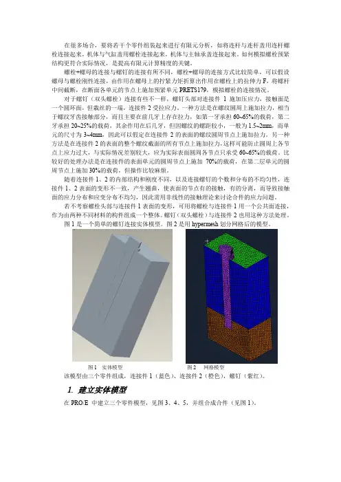
图1是一个简单的螺钉连接实体模型。

图2是用hypermesh 划分网格后的模型。

图1 实体模型 图2 网格模型该模型由三个零件组成，连接件1（蓝色）、连接件2（橙色），螺钉（紫红）。

HyperMesh梁单元和壳单元的混合建模本文根据工程实例，应用有限元软件HyperMesh 进行梁单元和壳单元的混合建模，并在其中详细论述，梁单元在与壳单元混合建模的过程中如何对梁单元进行偏置处理，保证梁单元与壳单元的所有节点完全耦合。

在焊接工艺中，梁单元与壳单元的使用可以大大提高整体焊接结构的抵抗变形能力，避免单独使用壳单元时强度和刚度的不足。

HyperMesh软件中提供了大量标准梁的截面，也可以通过实际应用需求单独创建梁截面。

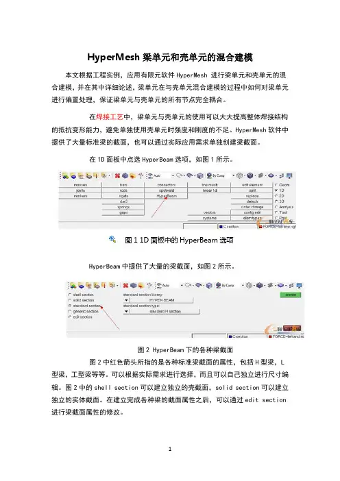
在1D面板中点选HyperBeam选项，如图1所示。

图1 1D面板中的HyperBeam选项HyperBeam中提供了大量的梁截面，如图2所示。

图2 HyperBeam下的各种梁截面图2中红色箭头所指的是各种标准梁截面的属性，包括H型梁，L 型梁，工型梁等等。

可以根据实际需求进行选择，而且可以自己独立进行尺寸编辑。

图2中的shell section可以建立独立的壳截面，solid section可以建立独立的实体截面。

在建立完成各种梁的截面属性之后，可以通过edit section 进行梁截面属性的修改。

以上主要介绍了1D梁单元的使用情况，下面将根据工程实例对壳单元和梁单元的混合建模进行详细的介绍。

图3是梁单元和壳单元焊接之后的三维图，图4是图3中梁单元以1D显示的情况。

二者之间的切换功能键如图5所示。

图3 梁单元和壳单元焊接之后梁单元以3D显示图4 梁单元和壳单元焊接之后梁单元以1D显示图5 梁单元1D与3D之间的切换功能键下面介绍梁单元的具体创建方法，不再讲述壳单元的建立方法。

首先建立Beam Section，在软件左侧右键create--Beam Section，在出现的对话框窗口中对Bean进行命名。

具体的过程如图6所示。

图6 Beam的建立过程之后进入1D--HyperBeam面板，选择Standard section选择Standard Channel面板，打开面板后对各个参数进行修改，如图7所示。

Hypermesh 资料-图文练习 2.2:创建材料集(MaterialCollector)1.在任何菜单页面上选择 collector 面板。

2.选择 create 子面板。

3.将 collector 的类型设置为 mat。

4.点击 name=并输入 teel。

5.将 creationmethod:设置为 cardimage=。

6.点击 cardimage=并选择 MAT1。

OptiStruct 模板支持四种材料类型MAT1、MAT2、MAT8 和 MAT9。

这些材料类型对应于相同的 NASTRAN 材料类型。

如果需要更多信息，请参考在线匡助中的 OptiStruct/DataFormat 部份。

7.点击 create/edit。

这一步就将 MAT1 这个 cardimage 赋给了这个新材料 teel。

如果某个输入域里没有值，表示当前相应的项是关闭的。

只要点击其标题就可以打开。

如果要在这个 cardimage 中为一个块输入一个值，点击相应的数据区域，然后输入数字。

8.点击 E，单击数据输入区并输入 2.0e5。

9.点击 NU，单击数据输入区并输入 0.30。

10.点击 return。

因为只需要做一个静态分析，所以没有必要定义一个密度值。

但是，在进行固有模态分析时，密度值就是必要的了。

这些二维单元被用来构造这个管状模型的实体单元。

2.点击 name=并输入 hell_elem。

5.点击 color 并从互动菜单中选择一个颜色。

1.点击 name=并输入 olid_elem。

2.将 creationmethod:设置为 cardimage=。

3.点击 cardimage=并从弹出菜单中选择 PSOLID。

4.点击 material=并选择 teel。

5.点击 color 并从弹出菜单中选择一个颜色。

6.点击 create 来创建这个 collector。

因为在 PSOLID 这个 card 中没有可以编辑的输入区域，就不用使用 create/edit 选项了。

Normal Modes Analysis of a Splash Shield - RD-1020In this tutorial, an existing finite element model of an automotive splash shield will be used to demonstrate how to set up and perform a normal modes analysis. HyperMesh post-processing tools are used to determine mode shapes of the model.The following exercises are included:•Retrieving the RADIOSS input file•Setting up the model in HyperMesh•Applying Loads and Boundary Conditions to the Model•Submitting the job•Viewing the resultsStep 1: Launch HyperMesh and set the RADIOSS (Bulk Data) User Profileunch HyperMesh.A User Profiles… Graphic User Interface (GUI) will appear. If it does not appear, go to Preferences►User Profiles … from the menu on the top.2.Select RADIOSS in the User Profile dialog.3.From the extended list, select Bulk Data.4.Click OK.This loads the User Profile. It includes the appropriate template, macro menu, and import reader, paring down the functionality of HyperMesh to what is relevant for generating models in Bulk Data Format for RADIOSS and OptiStruct.Step 2: Import a Finite Element Model File in HyperMesh1.From the File pull-down menu on the toolbar, select Import….An Import… tab is added to your tab menu.2.Click to import an FE model.3.For the File type:, select RADIOSS (Bulk Data).4.Select the Files icon button.A Select RADIOSS (Bulk Data) file browser will pop up.5.Browse for sshield.fem file located in the HyperWorks installation directory under<install_directory>/tutorials/hwsolvers/radioss/ and select the file.6.Click Open►Import.7.Click Close to close the Import tab menu.Step 3: Review Rigid ElementsNotice there are two rigid "spiders" in the model. They are placed at locations where the shield is bolted down. This is a simplified representation of the interaction between the bolts and the shield. It is assumed that the bolts are significantly more rigid in comparison to the shield.The dependent nodes of the rigid elements have all six degrees of freedom constrained. Therefore, each "spider" connects nodes of the shell mesh together in such a way that they do not move with respect to one another.The following steps show how to review the properties of the rigid elements.1.From the 1D page, select the rigids.2.Click review.3.Select one of the rigid elements in the graphics region.In the graphics window, HyperMesh displays the IDs of the rigid element and the two end nodes and indicates the independent node with an 'I' and the dependent node with a 'D'. HyperMesh also indicates the constrained degrees of freedom for the selected element, through the dof checkboxes in the rigids panel. All rigid elements in this model should have all dofs constrained.4.Click return to go to the main menu.Step 4: Setting up the Material and Geometric PropertiesThe imported model has three component collectors with no materials. A material collector needs to be created and assigned to the shell component collectors. The rigid elements do not need to be assigned a material. Shell thickness values also need to be corrected.1.Select the Material Collectors toolbar button .2.Select the create subpanel using the radio buttons on the left-hand side of the panel.3.Click mat name = and enter steel.4.Select the desired color for the material steel by clicking on .5.Click card image = and select MAT1 from the pop-up menu.6.Click create/edit.The MAT1 card image pops up.7.For E, enter the value 2.0E5.8.For NU, enter the value 0.3.9.For RHO, enter the value 7.85E-9.If a quantity in brackets does not have a value below it, it is off. To change this, click the quantity in brackets and an entry field will appear below it. Click in the entry field, and a value can be entered.10.Click return.A new material, steel, has now been created. The material uses RADIOSS linear isotropic materialmodel, MAT1. This material has a Young's Modulus of 2E+05, a Poisson's Ratio of 0.3 and a material density of 7.85E-09. A material density is required for the normal modes solution sequence.At any time the card image for this collector can be modified using Card Editor.11.Click return to exit the Material Create panel.12.Select the Card Editor toolbar button .13.Click the down arrow on the right of the entity shown in the yellow box, select props from the extendedentity list.14.Click the yellow props button and then check the box next to design and nondesign.15.Click select.16.Make sure card image=is set to PSHELL.17.Click edit.The PSHELL card image for the design component collector pops up.18.Replace 0.300 in the T field with 0.25.19.Click return to save the changes to the card image.20.Click return to go to the main menu.Applying Loads and Boundary Conditions to the Model (Steps 5 - 7)The model is to be constrained using SPCs at the bolt locations, as shown in the following figure. The constraints will be organized into the load collector 'constraints'.To perform a normal modes analysis, a real eigenvalue extraction (EIGRL) card needs to be referenced in the subcase. The real eigenvalue extraction card is defined in HyperMesh as a load collector with an EIGRL card image. This load collector should not contain any other loads.Step 5: Create EIGRL card (to request the number of modes)If a quantity in brackets does not have a value below it, it is off. To change this, click on the quantity in brackets and an entry field will appear below it. Click on the entry field, and a value can be entered.Step 6: Create Constraints at Bolt LocationsSelecting nodes for constraining the bolt locations 1.Click the Load Collectors toolbar button .2.Select the create subpanel, using the radio buttons on the left-hand side of the panel.3.Click loadcol name = and enter EIGRL .4.Click card image= and select EIGRL from the pop-up menu.5.Click create/edit .6.For V2, enter the value 200.000.7.For ND , enter the value 6.8.Click return to save changes to the card image.1.Click loadcol name = and enter constraints .2.Click the switch next to card image and select no card image .3.Click create > return .4.From Analysis page, click the constraints panel and make sure that the createsubpanel is active.5.Select the two nodes, shown in the figure above, at the center of the rigid spiders, by clicking on them in the graphics window.6.Constrain all dofs with a value of 0.0.7.Click Load Type= and select SPC .8.Click createTwo constraints are created. Constraint symbols (triangles) appear in the graphics window at theselected nodes. The number 123456 is written beside the constraint symbol, if the label constraints is checked ‘ON’, indicating that all dofs are constrained.9.Click return to go the main menu.Step 7: Create a Load Step to perform Normal Modes Analysis1.From the Analysis page, enter the loadsteps panel.2.Click name = and enter bolted.3.Click the type: switch and select normal modes from the pop-up menu.4.Check the box preceding SPC.An entry field appears to the right of SPC.5.Click on the entry field and select constraints from the list of load collectors.6.Check the box preceding METHOD(STRUCT).An entry field appears to the right of METHOD.7.Click on the entry field and select EIGRL from the list of load collectors.8.Click create.A RADIOSS subcase has been created which references the constraints in the load collector constraintsand the real eigenvalue extraction data in the load collector EIGRL.9.Click return to go to the main menu.Submitting the JobStep 8: Running Normal Modes Analysis1.From the Analysis page, enter the RADIOSS panel.2.Click save as… following the input file:field.A Save file… browser window pops up.3.Select the directory where you would like to write the file and, in File name:, entersshield_complete.fem.4.Click Save.Note that the name and location of the sshield_complete.fem file shows in the input file: field.5.Set the export options:toggle to all.6.Click the run options: switch and select analysis.7.Set the memory options: toggle to memory default.8.Click Radioss.This launches the RADIOSS job.If the job was successful, new results files can be seen in the directory where the RADIOSS model file was written. The sshield_complete.out file is a good place to look for error messages that will help to debug the input deck if any errors are present.The default files written to your directory are:sshield_complete.html HTML report of the analysis, giving a summary of the problemformulation and the analysis results.sshield_complete.out RADIOSS output file containing specific information on the file setup, the set up of your optimization problem, estimates for the amountof RAM and disk space required for the run, information for eachoptimization iteration, and compute time information. Review this fileReview the Results using HyperViewEigenvector results are output by default, from RADIOSS for a normal modes analysis. This section describes how to view the results in HyperView.Step 9: Load the Model and Result Files into the Animation WindowIn this section, you will load a HyperView .h3d file into the HyperView animation window.HyperView is launched and the sshield_complete.h3d file is loaded.Step 10: View Eigen VectorsIt is helpful to view the deformed shape of a model to determine if the boundary conditions have been defined correctly and also to check if the model is deforming as expected. In this section, use the Deformed panel to review the deformed shape for last Mode .This means that the maximum displacement will be 10 modal units and all other displacements will be proportional.Using a scale factor higher than 1.0 amplifies the deformations while a scale factor smaller than 1.0 would reduce them. In this case, we are accentuating displacements in all directions.A deformed plot of the model overlaid on the original undeformed mesh is displayed in the graphics window. for warnings and errors.sshield_complete.h3dHyper 3D binary results file. sshield_complete.stat Summary of analysis process, providing CPU information for eachstep during analysis process. 1.Click the HyperView button in the RADIOSS panel. 2.Click Close to exit the Message Log menu that appears.1.Click on the switch next to the traffic light signaland select Modal .2.Select the Deformed toolbar button.3.Leave Result type:set to Eigen Mode (v).4.Set Scale: to Model units .5.Set Type: to Uniform and enter in a scale factor of 10 for Value:.6.Click Apply .7.Under Undeformed shape:, set Show: to Wireframe .8.From the Graphics pull-down menu, select Select Load Case to activate the Load Case andSimulation Selection dialog, as shown below.Step 11: A few points to be notedIn this analysis, it was assumed that the bolts were significantly stiffer than the shield. If the bolts needed to be made of aluminum and the shield was still made of steel, would the model need to be modified, and the analysis run again?It is necessary to push the natural frequencies of the splash shield above 50 Hz. With the current model, there should be one mode that violates this constraint: Mode 1. Design specifications allow the innerdisjointed circular rib to be modified such that no significant mass is added to the part. Is there a configuration for this rib within the above stated constraints that will push the first mode above 50 Hz? See tutorial OS-2020 to optimize rib locations for this part.Go ToRADIOSS, MotionSolve, and OptiStruct Tutorials9.Select Mode 6 - F=1.496557E+02 from the list and click OK to view Mode 6.10.To animate the mode shape, click the animation mode: modal.11.To control the animation speed, use the Animation Controls accessed with the director’s chair toolbar button .12.You could also review the rest of the mode shapes.。

Normal Modes Analysis of a Splash Shield - RD-1020In this tutorial, an existing finite element model of an automotive splash shield will be used to demonstrate how to set up and perform a normal modes analysis. HyperMesh post-processing tools are used to determine mode shapes of the model.The following exercises are included:•Retrieving the RADIOSS input file•Setting up the model in HyperMesh•Applying Loads and Boundary Conditions to the Model•Submitting the job•Viewing the resultsStep 1: Launch HyperMesh and set the RADIOSS (Bulk Data) User Profileunch HyperMesh.A User Profiles… Graphic User Interface (GUI) will appear. If it does not appear, go to Preferences►User Profiles … from the menu on the top.2.Select RADIOSS in the User Profile dialog.3.From the extended list, select Bulk Data.4.Click OK.This loads the User Profile. It includes the appropriate template, macro menu, and import reader, paring down the functionality of HyperMesh to what is relevant for generating models in Bulk Data Format for RADIOSS and OptiStruct.Step 2: Import a Finite Element Model File in HyperMesh1.From the File pull-down menu on the toolbar, select Import….An Import… tab is added to your tab menu.2.Click to import an FE model.3.For the File type:, select RADIOSS (Bulk Data).4.Select the Files icon button.A Select RADIOSS (Bulk Data) file browser will pop up.5.Browse for sshield.fem file located in the HyperWorks installation directory under<install_directory>/tutorials/hwsolvers/radioss/ and select the file.6.Click Open►Import.7.Click Close to close the Import tab menu.Step 3: Review Rigid ElementsNotice there are two rigid "spiders" in the model. They are placed at locations where the shield is bolted down. This is a simplified representation of the interaction between the bolts and the shield. It is assumed that the bolts are significantly more rigid in comparison to the shield.The dependent nodes of the rigid elements have all six degrees of freedom constrained. Therefore, each "spider" connects nodes of the shell mesh together in such a way that they do not move with respect to one another.The following steps show how to review the properties of the rigid elements.1.From the 1D page, select the rigids.2.Click review.3.Select one of the rigid elements in the graphics region.In the graphics window, HyperMesh displays the IDs of the rigid element and the two end nodes and indicates the independent node with an 'I' and the dependent node with a 'D'. HyperMesh also indicates the constrained degrees of freedom for the selected element, through the dof checkboxes in the rigids panel. All rigid elements in this model should have all dofs constrained.4.Click return to go to the main menu.Step 4: Setting up the Material and Geometric PropertiesThe imported model has three component collectors with no materials. A material collector needs to be created and assigned to the shell component collectors. The rigid elements do not need to be assigned a material. Shell thickness values also need to be corrected.1.Select the Material Collectors toolbar button .2.Select the create subpanel using the radio buttons on the left-hand side of the panel.3.Click mat name = and enter steel.4.Select the desired color for the material steel by clicking on .5.Click card image = and select MAT1 from the pop-up menu.6.Click create/edit.The MAT1 card image pops up.7.For E, enter the value 2.0E5.8.For NU, enter the value 0.3.9.For RHO, enter the value 7.85E-9.If a quantity in brackets does not have a value below it, it is off. To change this, click the quantity in brackets and an entry field will appear below it. Click in the entry field, and a value can be entered.10.Click return.A new material, steel, has now been created. The material uses RADIOSS linear isotropic materialmodel, MAT1. This material has a Young's Modulus of 2E+05, a Poisson's Ratio of 0.3 and a material density of 7.85E-09. A material density is required for the normal modes solution sequence.At any time the card image for this collector can be modified using Card Editor.11.Click return to exit the Material Create panel.12.Select the Card Editor toolbar button .13.Click the down arrow on the right of the entity shown in the yellow box, select props from the extendedentity list.14.Click the yellow props button and then check the box next to design and nondesign.15.Click select.16.Make sure card image=is set to PSHELL.17.Click edit.The PSHELL card image for the design component collector pops up.18.Replace 0.300 in the T field with 0.25.19.Click return to save the changes to the card image.20.Click return to go to the main menu.Applying Loads and Boundary Conditions to the Model (Steps 5 - 7)The model is to be constrained using SPCs at the bolt locations, as shown in the following figure. The constraints will be organized into the load collector 'constraints'.To perform a normal modes analysis, a real eigenvalue extraction (EIGRL) card needs to be referenced in the subcase. The real eigenvalue extraction card is defined in HyperMesh as a load collector with an EIGRL card image. This load collector should not contain any other loads.Step 5: Create EIGRL card (to request the number of modes)If a quantity in brackets does not have a value below it, it is off. To change this, click on the quantity in brackets and an entry field will appear below it. Click on the entry field, and a value can be entered.Step 6: Create Constraints at Bolt LocationsSelecting nodes for constraining the bolt locations 1.Click the Load Collectors toolbar button .2.Select the create subpanel, using the radio buttons on the left-hand side of the panel.3.Click loadcol name = and enter EIGRL .4.Click card image= and select EIGRL from the pop-up menu.5.Click create/edit .6.For V2, enter the value 200.000.7.For ND , enter the value 6.8.Click return to save changes to the card image.1.Click loadcol name = and enter constraints .2.Click the switch next to card image and select no card image .3.Click create > return .4.From Analysis page, click the constraints panel and make sure that the createsubpanel is active.5.Select the two nodes, shown in the figure above, at the center of the rigid spiders, by clicking on them in the graphics window.6.Constrain all dofs with a value of 0.0.7.Click Load Type= and select SPC .8.Click createTwo constraints are created. Constraint symbols (triangles) appear in the graphics window at theselected nodes. The number 123456 is written beside the constraint symbol, if the label constraints is checked ‘ON’, indicating that all dofs are constrained.9.Click return to go the main menu.Step 7: Create a Load Step to perform Normal Modes Analysis1.From the Analysis page, enter the loadsteps panel.2.Click name = and enter bolted.3.Click the type: switch and select normal modes from the pop-up menu.4.Check the box preceding SPC.An entry field appears to the right of SPC.5.Click on the entry field and select constraints from the list of load collectors.6.Check the box preceding METHOD(STRUCT).An entry field appears to the right of METHOD.7.Click on the entry field and select EIGRL from the list of load collectors.8.Click create.A RADIOSS subcase has been created which references the constraints in the load collector constraintsand the real eigenvalue extraction data in the load collector EIGRL.9.Click return to go to the main menu.Submitting the JobStep 8: Running Normal Modes Analysis1.From the Analysis page, enter the RADIOSS panel.2.Click save as… following the input file:field.A Save file… browser window pops up.3.Select the directory where you would like to write the file and, in File name:, entersshield_complete.fem.4.Click Save.Note that the name and location of the sshield_complete.fem file shows in the input file: field.5.Set the export options:toggle to all.6.Click the run options: switch and select analysis.7.Set the memory options: toggle to memory default.8.Click Radioss.This launches the RADIOSS job.If the job was successful, new results files can be seen in the directory where the RADIOSS model file was written. The sshield_complete.out file is a good place to look for error messages that will help to debug the input deck if any errors are present.The default files written to your directory are:sshield_complete.html HTML report of the analysis, giving a summary of the problemformulation and the analysis results.sshield_complete.out RADIOSS output file containing specific information on the file setup, the set up of your optimization problem, estimates for the amountof RAM and disk space required for the run, information for eachoptimization iteration, and compute time information. Review this fileReview the Results using HyperViewEigenvector results are output by default, from RADIOSS for a normal modes analysis. This section describes how to view the results in HyperView.Step 9: Load the Model and Result Files into the Animation WindowIn this section, you will load a HyperView .h3d file into the HyperView animation window.HyperView is launched and the sshield_complete.h3d file is loaded.Step 10: View Eigen VectorsIt is helpful to view the deformed shape of a model to determine if the boundary conditions have been defined correctly and also to check if the model is deforming as expected. In this section, use the Deformed panel to review the deformed shape for last Mode .This means that the maximum displacement will be 10 modal units and all other displacements will be proportional.Using a scale factor higher than 1.0 amplifies the deformations while a scale factor smaller than 1.0 would reduce them. In this case, we are accentuating displacements in all directions.A deformed plot of the model overlaid on the original undeformed mesh is displayed in the graphics window. for warnings and errors.sshield_complete.h3dHyper 3D binary results file. sshield_complete.stat Summary of analysis process, providing CPU information for eachstep during analysis process. 1.Click the HyperView button in the RADIOSS panel. 2.Click Close to exit the Message Log menu that appears.1.Click on the switch next to the traffic light signaland select Modal .2.Select the Deformed toolbar button.3.Leave Result type:set to Eigen Mode (v).4.Set Scale: to Model units .5.Set Type: to Uniform and enter in a scale factor of 10 for Value:.6.Click Apply .7.Under Undeformed shape:, set Show: to Wireframe .8.From the Graphics pull-down menu, select Select Load Case to activate the Load Case andSimulation Selection dialog, as shown below.Step 11: A few points to be notedIn this analysis, it was assumed that the bolts were significantly stiffer than the shield. If the bolts needed to be made of aluminum and the shield was still made of steel, would the model need to be modified, and the analysis run again?It is necessary to push the natural frequencies of the splash shield above 50 Hz. With the current model, there should be one mode that violates this constraint: Mode 1. Design specifications allow the innerdisjointed circular rib to be modified such that no significant mass is added to the part. Is there a configuration for this rib within the above stated constraints that will push the first mode above 50 Hz? See tutorial OS-2020 to optimize rib locations for this part.Go ToRADIOSS, MotionSolve, and OptiStruct Tutorials9.Select Mode 6 - F=1.496557E+02 from the list and click OK to view Mode 6.10.To animate the mode shape, click the animation mode: modal.11.To control the animation speed, use the Animation Controls accessed with the director’s chair toolbar button .12.You could also review the rest of the mode shapes.。