Iterative methods for nonlinear operator equations

(Stoer & Bulirsch, Cheney & Kincaid)
1. Methods for initial value problems for ordinary di erential equations: Runge-Kutta and Adams methods.
2. Methods with automatic step-size control for Runge-Kutta and Adams methods. 3. Basic concepts of stability of the multistep methods for ODE's and systems.
7. Finite element method
(Joix)
1. Weak (variational) formulation and characterization of the energy space: essential and natural boundary condition.
3. Eigenvalues and eigenvectors of matrices (minimax methods for symmetric matrices, power method, QR method). Singular value decomposition and its basic properties.
estimates (Courant condition). 3. Error estimates
6. Numerical methods for elliptic problems
(Ames, Striktwerda)
1. Finite di erences and nite volumes: approximation of the equation and the boundary conditions, higher order schemes.

非线性方程重根的三阶迭代方法李福祥;田金燕;费兆福;巩英海;曹作宝【摘要】为提高求解非线性方程的收敛速度和计算效率,以牛顿法为基础提出一种求解非线性方程重根的迭代方法,该方法以重数已知为前提,迭代格式根据重数为奇数和偶数两种情形分别给出,两种迭代格式每步迭代都只需计算三个函数值(包含一阶导数值)且完全摆脱了二阶导数值的计算,其收敛效果皆可达到三阶.算例实验结果验证了该迭代方法的有效性.他丰富了非线性方程求根的方法,在理论上和应用上都有一定的价值.【期刊名称】《哈尔滨理工大学学报》【年(卷),期】2013(018)006【总页数】4页(P117-120)【关键词】非线性方程;牛顿法;重根;迭代法;三阶收敛【作者】李福祥;田金燕;费兆福;巩英海;曹作宝【作者单位】哈尔滨理工大学应用科学学院,黑龙江哈尔滨 150080;哈尔滨理工大学应用科学学院,黑龙江哈尔滨 150080;哈尔滨理工大学应用科学学院,黑龙江哈尔滨 150080;哈尔滨理工大学应用科学学院,黑龙江哈尔滨 150080;哈尔滨理工大学应用科学学院,黑龙江哈尔滨 150080【正文语种】中文【中图分类】O24求解非线性方程f(x)=0是数学界经久不衰的研究课题，究其原因就是其在科学研究以及生产生活中的广泛应用，而迭代法又是求解非线性方程最为常用的方法之一．本文着重研究求解非线性方程重根的情形．寻找非线性方程重根的迭代方法通常以重数已知为前提，最为经典的当属二阶收敛的Newton迭代法，为提高其收敛速度一系列高阶迭代方法得到人们的广泛研究，这些方法大多是三阶收敛的，大致可分为两类，一类叫做单点法每步迭代需要计算三个函数值分别是 f，f'，和f″，比如欧拉－切比雪夫方法［1－2］哈雷方法［3］，Chun and Neta 方法［4］，Biazar and Ghanbari法［5］，和 Osada 法［6］等都属于此类，此类方法相比于经典的Newton法收敛效率大幅提高，但是每部迭代需要计算二阶导数值，这无疑增加了迭代过程的复杂度;另一类叫做多点法(本文的方法属此类)又可以被分成两子类，一个子类需要计算两个函数值和一个一阶导数值，比如文［7］，文［9］，文［10］等人给出的方法，另一子类需要计算两个一阶导数值和一个函数值，比如文［11－14］等人给出的方法，此类方法不仅提高了收敛速率，计算量也得到了很好的控制．再次就是四阶收敛的迭代方法，例如文［15－18］等人提出的方法，增加一个函数计算(f或f')将收敛速率提高到了四阶．由于受到上述研究工作的启发，为提高求解非线性方程的收敛速度和计算效率，本文以牛顿法为基础提出一种求解非线性方程重根的迭代方法，迭代格式根据重数为奇数和偶数两种情形分别给出，两种迭代格式每步迭代都只需计算三个函数值(包含一阶导数值)且完全摆脱了二阶导数值的计算，其收敛效果皆可达到三阶．正如引言中所提到的，本文的迭代方法同样以重数m已知为前提，当m为奇数时迭代格式如下所示:从迭代格式可以发现，不管重数是奇数还是偶数，每步迭代都仅需计算三个函数值，接下来我们将给出其收敛性证明．定理设x*∈D是充分光滑的实值函数f:D⊆R→R在开区间D上的m重根，当x0∈D充分靠近x*时，由式(1)、(2)决定的迭代方法至少是三阶收敛的．注意到，无论重数m是奇数还是偶数，由式(1)、(2)决定的三阶迭代方法每步迭代都只需计算三个函数值．其效率指数为，这里p指代收敛阶数，c指代所需计算函数个数．在这里将本文给出的方法应用到如下数值算例中，为展示本文迭代方法的属性及可行性，我们将从引言中提到的两类三阶迭代法中分别挑选出四种方法与本文迭代法(用M代表)做对比，SM(属单点法，需计算 f，f'，和f″)代表文［14］提出的迭代法，HMM(需计算 f，f，f')出自于文［10］，LM － 1(同HMM)和 LM －2(需计算 f，f'，f')都出自文献［12］．所有的数学计算都将用数学软件Mathematica完成，选择|x－x*|≤10－100作为终止条件．数值计算结果将呈现在表1中，其中en保留五位有效小数，n表示迭代次数．2)f2=ex－2+1 －x，f2(x)=0 有 2 重根 x*=2，选择x0=2.4为初始值;3)f3(x)=sin［(x－3)5］，f3(x)=0有 5重根x*=3，选择x0=2.5为初始值．4)f4(x)=(x－1)(ex－1－1)，f4(x)=0 有 2 重根x*=1，选择x0=1.5为初值．从表1中可以看出，本文构造的迭代方法M与同收敛阶的其他方法SM，HMM，LM－1，LM－2均能以较快的速度收敛．由算例可以明显发现本文提出的迭代方法是三阶收敛的．田金燕(1988—)，女，硕士研究生;费兆福(1989—)，男，硕士研究生．【相关文献】［1］TRAUB J F．Iterative Methods for the Solution of Equations［M］．NJ，Prentice-Hall:Englewood Cliffs，1964:10 －85．［2］NETA B．New Third Order Nonlinear Solvers for Multiple Roots，Appl ［J］．Math．Comput．，2008，202:162 －170．［3］HALLEY E．A New Exact and Easy Method of Finding the Roots of Equations Generally and without any Previous Reduction［J］．Phil．Trans．Roy．Soc．Lori．，1694，18:136 －148．［4］CHUN C，Neta B．A Third Order Modification of Newton’s Method for Multiple Roots［J］．Appl．Math．Comput．，2009，211:474－479．［5］BIAZAR J，GHANBARI B．A New third-order Family of Nonlinear Solvers for Multiple Roots［J］．Comput．Math．Appl．，2010，59:3315－3319．［6］OSADA N．An Optimal Multiple Root-finding Method of Order Three ［J］．Comput．Appl．Math．，1994，51:131 －133．［7］DONG C．A Basic Theorem of Constructing an Iiterative Formula of the Higher Order for Computing Multiple Roots of an Equation［J］．Math．Numer．Sinica，1982，11:445 －450．［8］NETA B．New Third Order Nonlinear Solvers for Multiple Roots ［J］．Appl．Math．Comput．，2008，202:162 － 170．［9］CHUN C，Bae H，Neta B．New Families of Nonlinear Third-order Solvers for Finding Multiple Roots［J］．Comput．Math．Appl．，2009，57:1574－1582．［10］HOMEIER H H H．On Newton-type Methods for Multiple Roots with Cubic Convergence ［J］．Comput．Appl．Math．，2009，231:249－254．［11］DONG C．A Family of Multipoint Iterative Functions for Finding Multiple Roots of Equations ［J］．Int．J．Comput．Math．，1987，21:363－367．［12］LI S，LI H，CHENG L．Some Second-derative-free Variants of Halley’s Method for Multiple Roots［J］．Appl．Math．Comput．，2009，215:2192 －2198．［13］SHARMA J R，SHARMA R．New Third and Fourth Order Nonlinear Solvers for Computing Multiple Roots［J］．Appl．Math．Comput，2011，217:9756 －9764．［14］SHARMA J R，SHARMA R．Modified Chebyshev-Hally Type Method and Its Variants for Computing Mmultiple Roots［J］．Numer Algor，2012，61:567 －578．［15］LI S，CHENG L，NETA B．Some Fourth-order Nonlinear Solvers with Closed Formulae for Multiple Roots ［J］．Comput．Math．Appl．，2010，59:126 －135．［16］NETA B．Extension of Murakami’s high-order Nonlinear Solver to Multiple Roots ［J］．Int．J．Comput．Math，2010，87:1023 －1031．［17］NETA B，JOHNSON A N．High Order Nonlinear Solver for Multiple Roots ［J］．Comput．Math．Appl，2008，55:2012 －2017．［18］SHARMA J R，SHARMA R．New Third and Rourth Order Nonlinear Solvers for Computingmultiple Roots［J］．Appl．Math．Comput，2011，217:9756 －9764．。

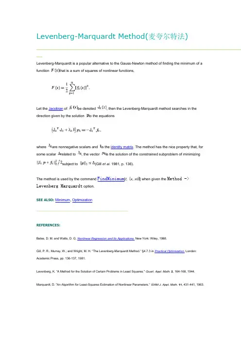
Levenberg-Marquardt Method(麦夸尔特法)Levenberg-Marquardt is a popular alternative to the Gauss-Newton method of finding the minimum of afunction that is a sum of squares of nonlinear functions,Let the Jacobian of be denoted , then the Levenberg-Marquardt method searches in thedirection given by the solution to the equationswhere are nonnegative scalars and is the identity matrix. The method has the nice property that, forsome scalar related to , the vector is the solution of the constrained subproblem of minimizingsubject to (Gill et al. 1981, p. 136).The method is used by the command FindMinimum[f, x, x0] when given the Method -> Levenberg Marquardt option.SEE A LSO:Minimum, OptimizationREFERENCES:Bates, D. M. and Watts, D. G. N onlinear Regr ession and Its Applications. New York: Wiley, 1988.Gill, P. R.; Murray, W.; and Wright, M. H. "The Levenberg-Marquardt Method." §4.7.3 in Practical Optim ization. London: Academic Press, pp. 136-137, 1981.Levenberg, K. "A Method for the Solution of Certain Problems in Least Squares." Quart. Appl. Math.2, 164-168, 1944. Marquardt, D. "An Algor ithm for Least-Squares Estimation of Nonlinear Parameters." SIAM J. Appl. Math.11, 431-441, 1963.Levenberg–Marquardt algorithmFrom Wikipedia, the free encyclopediaJump to: navigation, searchIn mathematics and computing, the Levenberg–Marquardt algorithm (LMA)[1] provides a numerical solution to the problem of minimizing a function, generally nonlinear, over a space of parameters of the function. These minimization problems arise especially in least squares curve fitting and nonlinear programming.The LMA interpolates between the Gauss–Newton algorithm (GNA) and the method of gradient descent. The LMA is more robust than the GNA, which means that in many cases it finds a solution even if it starts very far off the final minimum. For well-behaved functions and reasonable starting parameters, the LMA tends to be a bit slower than the GNA. LMA can also be viewed as Gauss–Newton using a trust region approach.The LMA is a very popular curve-fitting algorithm used in many software applications for solving generic curve-fitting problems. However, the LMA finds only a local minimum, not a global minimum.Contents[hide]∙ 1 Caveat Emptor∙ 2 The problem∙ 3 The solutiono 3.1 Choice of damping parameter∙ 4 Example∙ 5 Notes∙ 6 See also∙7 References∙8 External linkso8.1 Descriptionso8.2 Implementations[edit] Caveat EmptorOne important limitation that is very often over-looked is that it only optimises for residual errors in the dependant variable (y). It thereby implicitly assumes that any errors in the independent variable are zero or at least ratio of the two is so small as to be negligible. This is not a defect, it is intentional, but it must be taken into account when deciding whether to use this technique to do a fit. While this may be suitable in context of a controlled experiment there are many situations where this assumption cannot be made. In such situations either non-least squares methods should be used or the least-squares fit should be done in proportion to the relative errors in the two variables, not simply the vertical "y" error. Failing to recognise this can lead to a fit which is significantly incorrect and fundamentally wrong. It will usually underestimate the slope. This may or may not be obvious to the eye.MicroSoft Excel's chart offers a trend fit that has this limitation that is undocumented. Users often fall into this trap assuming the fit is correctly calculated for all situations. OpenOffice spreadsheet copied this feature and presents the same problem.[edit] The problemThe primary application of the Levenberg–Marquardt algorithm is in the least squares curve fitting problem: given a set of m empirical datum pairs of independent and dependent variables, (x i, y i), optimize the parameters β of the model curve f(x,β) so that the sum of the squares of the deviationsbecomes minimal.[edit] The solutionLike other numeric minimization algorithms, the Levenberg–Marquardt algorithm is an iterative procedure. To start a minimization, the user has to provide an initial guess for the parameter vector, β. In many cases, an uninformed standard guess like βT=(1,1,...,1) will work fine;in other cases, the algorithm converges only if the initial guess is already somewhat close to the final solution.In each iteration step, the parameter vector, β, is replaced by a new estimate, β + δ. To determine δ, the functions are approximated by their linearizationswhereis the gradient(row-vector in this case) of f with respect to β.At its minimum, the sum of squares, S(β), the gradient of S with respect to δwill be zero. The above first-order approximation of gives.Or in vector notation,.Taking the derivative with respect to δand setting theresult to zero gives:where is the Jacobian matrix whose i th row equals J i,and where and are vectors with i th componentand y i, respectively. This is a set of linear equations which can be solved for δ.Levenberg's contribution is to replace this equation by a "damped version",where I is the identity matrix, giving as the increment, δ, to the estimated parameter vector, β.The (non-negative) damping factor, λ, isadjusted at each iteration. If reduction of S is rapid, a smaller value can be used, bringing the algorithm closer to the Gauss–Newton algorithm, whereas if an iteration gives insufficientreduction in the residual, λ can be increased, giving a step closer to the gradient descentdirection. Note that the gradient of S withrespect to β equals .Therefore, for large values of λ, the step will be taken approximately in the direction of the gradient. If either the length of the calculated step, δ, or the reduction of sum of squares from the latest parameter vector, β + δ, fall below predefined limits, iteration stops and the last parameter vector, β, is considered to be the solution.Levenberg's algorithm has the disadvantage that if the value of damping factor, λ, is large, inverting J T J + λI is not used at all. Marquardt provided the insight that we can scale eachcomponent of the gradient according to thecurvature so that there is larger movement along the directions where the gradient is smaller. This avoids slow convergence in the direction of small gradient. Therefore, Marquardt replaced theidentity matrix, I, with the diagonal matrixconsisting of the diagonal elements of J T J,resulting in the Levenberg–Marquardt algorithm:.A similar damping factor appears in Tikhonov regularization, which is used to solve linear ill-posed problems, as well as in ridge regression, an estimation technique in statistics.[edit] Choice of damping parameterVarious more-or-less heuristic arguments have been put forward for the best choice for the damping parameter λ. Theoretical arguments exist showing why some of these choices guaranteed local convergence of the algorithm; however these choices can make the global convergence of the algorithm suffer from the undesirable properties of steepest-descent, in particular very slow convergence close to the optimum.The absolute values of any choice depends on how well-scaled the initial problem is. Marquardt recommended starting with a value λ0 and a factor ν>1. Initially setting λ=λ0and computing the residual sum of squares S(β) after one step from the starting point with the damping factor of λ=λ0 and secondly withλ0/ν. If both of these are worse than the initial point then the damping is increased by successive multiplication by νuntil a better point is found with a new damping factor of λ0νk for some k.If use of the damping factor λ/ν results in a reduction in squared residual then this is taken as the new value of λ (and the new optimum location is taken as that obtained with this damping factor) and the process continues; if using λ/ν resulted in a worse residual, but using λresulted in a better residual then λ is left unchanged and the new optimum is taken as the value obtained with λas damping factor.[edit] ExamplePoor FitBetter FitBest FitIn this example we try to fit the function y = a cos(bX) + b sin(aX) using theLevenberg–Marquardt algorithm implemented in GNU Octave as the leasqr function. The 3 graphs Fig 1,2,3 show progressively better fitting for the parameters a=100, b=102 used in the initial curve. Only when the parameters in Fig 3 are chosen closest to the original, are thecurves fitting exactly. This equation is an example of very sensitive initial conditions for the Levenberg–Marquardt algorithm. One reason for this sensitivity is the existenceof multiple minima —the function cos(βx)has minima at parameter value and[edit] Notes1.^ The algorithm was first published byKenneth Levenberg, while working at theFrankford Army Arsenal. It was rediscoveredby Donald Marquardt who worked as astatistician at DuPont and independently byGirard, Wynn and Morrison.[edit] See also∙Trust region[edit] References∙Kenneth Levenberg(1944). "A Method for the Solution of Certain Non-Linear Problems in Least Squares". The Quarterly of Applied Mathematics2: 164–168.∙ A. Girard (1958). Rev. Opt37: 225, 397. ∙ C.G. Wynne (1959). "Lens Designing by Electronic Digital Computer: I". Proc.Phys. Soc. London73 (5): 777.doi:10.1088/0370-1328/73/5/310.∙Jorje J. Moré and Daniel C. Sorensen (1983)."Computing a Trust-Region Step". SIAM J.Sci. Stat. Comput. (4): 553–572.∙ D.D. Morrison (1960). Jet Propulsion Laboratory Seminar proceedings.∙Donald Marquardt (1963). "An Algorithm for Least-Squares Estimation of NonlinearParameters". SIAM Journal on AppliedMathematics11 (2): 431–441.doi:10.1137/0111030.∙Philip E. Gill and Walter Murray (1978)."Algorithms for the solution of thenonlinear least-squares problem". SIAMJournal on Numerical Analysis15 (5):977–992. doi:10.1137/0715063.∙Nocedal, Jorge; Wright, Stephen J. (2006).Numerical Optimization, 2nd Edition.Springer. ISBN0-387-30303-0.[edit] External links[edit] Descriptions∙Detailed description of the algorithm can be found in Numerical Recipes in C, Chapter15.5: Nonlinear models∙ C. T. Kelley, Iterative Methods for Optimization, SIAM Frontiers in AppliedMathematics, no 18, 1999, ISBN0-89871-433-8. Online copy∙History of the algorithm in SIAM news∙ A tutorial by Ananth Ranganathan∙Methods for Non-Linear Least Squares Problems by K. Madsen, H.B. Nielsen, O.Tingleff is a tutorial discussingnon-linear least-squares in general andthe Levenberg-Marquardt method inparticular∙T. Strutz: Data Fitting and Uncertainty (A practical introduction to weighted least squares and beyond). Vieweg+Teubner, ISBN 978-3-8348-1022-9.[edit] Implementations∙Levenberg-Marquardt is a built-in algorithm with Mathematica∙Levenberg-Marquardt is a built-in algorithm with Matlab∙The oldest implementation still in use is lmdif, from MINPACK, in Fortran, in thepublic domain. See also:o lmfit, a translation of lmdif into C/C++ with an easy-to-use wrapper for curvefitting, public domain.o The GNU Scientific Library library hasa C interface to MINPACK.o C/C++ Minpack includes theLevenberg–Marquardt algorithm.o Several high-level languages andmathematical packages have wrappers forthe MINPACK routines, among them:▪Python library scipy, modulescipy.optimize.leastsq,▪IDL, add-on MPFIT.▪R (programming language) has theminpack.lm package.∙levmar is an implementation in C/C++ with support for constraints, distributed under the GNU General Public License.o levmar includes a MEX file interface for MATLABo Perl (PDL), python and Haskellinterfaces to levmar are available: seePDL::Fit::Levmar, PyLevmar andHackageDB levmar.∙sparseLM is a C implementation aimed at minimizing functions with large,arbitrarily sparse Jacobians. Includes a MATLAB MEX interface.∙ALGLIB has implementations of improved LMA in C# / C++ / Delphi / Visual Basic.Improved algorithm takes less time toconverge and can use either Jacobian orexact Hessian.∙NMath has an implementation for the .NET Framework.∙gnuplot uses its own implementation .∙Java programming language implementations:1) Javanumerics, 2) LMA-package (a small,user friendly and well documentedimplementation with examples and support),3) Apache Commons Math∙OOoConv implements the L-M algorithm as an Calc spreadsheet.∙SAS, there are multiple ways to access SAS's implementation of the Levenberg-Marquardt algorithm: it can be accessed via NLPLMCall in PROC IML and it can also be accessed through the LSQ statement in PROC NLP, and the METHOD=MARQUARDT option in PROC NLIN.。

The Sequential Quadratic Programming Method
167
2 ewton Methods and Local Optimality
In this and subsequent sections we trace the development of Newton methods from the simplest case of nonlinear equations, through to the general case of nonlinear programming with equations and inequalities.
x∈IR
subject to ci (x) ≥ 0
i = 1 , 2 , . . . , m.
(1.1)
In this formulation, equation constraints must be encoded as two opposed inequality constraints, that is c(x) = 0 is replaced by c(x) ≥ 0 and −c(x) ≥ 0, which is usually not convenient. Thus in practice a more detailed formulation is appropriate, admitting also equations, linear constraints and simple bounds. One way to do this is to add slack variables to the constraints, which
The Sequential Quadratic Programming Method